Glyphs for Space-Time Jacobians of Time-Dependent
Vector Fields
Tim Gerrits Christian Rössl Holger Theisel
Visual Computing Group, University of Magdeburg {gerrits|roessl|theisel}@isg.cs.uni-magdeburg.de
ABSTRACT
Glyphs have proven to be a powerful visualization technique for general tensor fields modeling physical phenom-ena such as diffusion or the derivative of flow fields. Most glyph constructions, however, do not provide a way of considering the temporal derivative, which is generally nonzero in non-stationary vector fields. This derivative offers a deeper understanding of features in time-dependent vector fields. We introduce an extension to 2D and 3D tensor glyph design that additionally encodes the temporal information of velocities, and thus makes it possible to represent time-dependent Jacobians. At the same time, a certain set of requirements for general tensor glyphs is fulfilled, such that the new method provides a visualization of the steadiness or unsteadiness of a vector field at a given instance of time.
Keywords
Tensor Glyphs, Glyph Design, Flow Visualization
1
INTRODUCTION
Glyphs have gained popularity as a tool for investigat-ing second-order tensors and their properties. They of-fer a convenient way to represent some of the under-lying physical meaning encoded in tensors such as dif-fusion or stress tensors at a given location in the data. The Jacobian matrix J of velocity fields is a second-order tensor, which appears in flow visualization and describes the local behavior of the flow at a given loca-tion, possibly in space-time. Unlike diffusion tensors, the second-order tensor Jacobians appear as general square matrices, including in particular non-symmetric matrices. This is generally a 2×2 matrix in 2D space, or 3×3 in 3D that consists of the spatial partial derivatives. Finding appropriate visualization techniques to rep-resent these matrices has proven to be a challenging task. Seltzer and Kindlmann [11] proposed the first glyphs for 2D tensor data that are able to represent any second-order tensor using the information encoded by eigenvalues and eigenvectors. Recently, Gerrits et al. [3] proposed a construction of glyphs for 2D tensors, which was then extended to visualize general 3D tensors as well. However, considering the special case of time-dependent Jacobian matrices, both approaches
Permission to make digital or hard copies of all or part of this work for personal or classroom use is granted without fee provided that copies are not made or distributed for profit or commercial advantage and that copies bear this notice and the full citation on the first page. To copy otherwise, or re-publish, to post on servers or to redistribute to lists, requires prior specific permission and/or a fee.
only deal with spatial derivatives and neglect temporal information that might be available.
In this paper, we solve the following problem: given ann-dimensional (n=2,3) time-dependent vector field
v(x,t), we construct an n-dimensional glyph that en-codes thespace-timeJacobian matrix ofv, i.e., all first order derivatives, both spatial and temporal, ofv. This means that we have to find a glyph representation for a
(n+1)×(n+1)Jacobian tensor. While this is straight-forward forn=2 (ending up in visualizing a 3×3 ma-trix), it is challenging for n=3 because this requires the 3D visualization of a 4×4 space-time Jacobian ten-sor. We show that this tensor, which is not a general 4D second-order tensor, has some properties that allow a 3D glyph visualization that seamlessly extends existing 3D tensor glyphs.
After analyzing related work in section 2, we present an extension of an existing second-order tensor glyph con-struction in section 3 that includes the temporal deriva-tive and therefore offers, to the best of our knowledge, the first glyph for time-dependent 2D and 3D Jacobians. This extension is constructed to in no way impair the glyph’s capability to encode the spatial derivatives. It becomes invisible, when the temporal derivative van-ishes. In this case, the resulting glyphs become identi-cal to time-independent tensor glyphs.
The results shown in section 4 present our final glyph designs for 2D and 3D time-dependent Jacobians. Ap-plying them on sampled locations demonstrates how the resulting glyphs additionally encode the temporal derivative of given time-dependent vector fields.
2
RELATED WORK AND
BACK-GROUND
2.1
Tensor Glyphs Visualization
Using visualization of flow fields to gain further insight of the underlying behavior has produced a huge variety of techniques that can coarsely be classified in differ-ent groups: topology-based techniques [9], dense flow visualization [7], geometric flow visualization [8] and glyph-based approaches. Glyphs are a convenient vi-sualization technique, as they are often tailored to fit a specific application and offer a seemingly unlimited design space, see Boro et al. [1]. Research trying to de-velop glyphs for second-order tensors has mostly been limited to symmetric positive definite matrices. The pioneering work by Schultz and Kindlmann [10] uses superquadrics to create glyphs, where shape and orien-tation are defined by the eigenvectors of general sym-metric tensors, including indefinite matrices. This is convenient, as eigenvectors of symmetric matrices are always orthogonal and therefore easily usable to define appropriate shapes. A general discussion on different approaches has been given by Kratz et al. [6]. Seltzer and Kindlmann [11] recently presented glyphs for gen-eral – symmetric and asymmetric – second-order 2D tensors, extending the superquadrics. Gerrits et al. [3] propose a different approach that provides glyphs also for general second-order tensors in 3D. Both works of-fer an in-depth discussion of tensor properties and de-sign principles leading to a set of requirements for a suitable glyph which will be covered in more detail in the next section.
As opposed to steady flows, time-dependent flow fields are only sparsely covered by glyph-based approaches. Often pathlines of a finite set of seed points are used to visualize flow in this case. Especially in topology-based visualization techniques, several works have been proposed, where the path of features over time is visu-alized as presented by Uffinger and Sadlo [13]. And even though there exist several approaches that try to extract only meaningful selections to give further in-sight [14, 4], there is still often visual clutter, overlap-ping elements or missing information by only rendering selected features. Hlawatsch et al. [5] downscale path-lines to represent them as so called pathline glyphs thus combining both techniques to address this problem.
2.2
Glyph Construction
Schultz and Kindlmann [10] present a set of construc-tion principles to build glyphs for symmetric tensors, which includes preservation of symmetry, continuity,
disambiguity, invariance under scaling as well as
eigenplane projection. The last requirement, however, is not well defined for asymmetric tensors, which is why Gerrits et al. [3] present a similar set of properties, but the latter is replaced by the demand for direct
encoding of real eigenvalues and eigenvectors. As these properties also influence the choices made in this paper, they are listed and explained in short:
(a)Invariance under isometric domain transformation: any isometric transformation of the domain should re-sult in the same isometric transformation of the glyph’s shape.
(b)Scaling invariance: a uniform scaling of the tensor has to result in the same scaling of the glyph for any real positive scaling value.
(c)Direct encoding of real eigenvalues and eigenvec-tors: all real eigenvalues and eigenvectors of the tensor should be directly visible within the shape of the glyph. (d) Uniqueness: a tensor should be represented by a unique corresponding glyph and vice-versa, such that for any two dissimilar tensors no similar glyph is pro-duced and no dissimilar glyphs are propro-duced by the same tensor.
(e) Continuity: any continuous change of the tensor should result in a continuous change of the glyph, pre-venting abrupt alterations of the appearance for small changes.
A glyph that satisfies all of these properties cannot be encoded by shape alone, but also needs at least one ad-ditional channel such as color.
(a) (b)
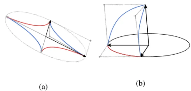
Figure 1: Basic glyph construction. (a) In 2D, each pair of scaled eigenvectors ( ) is interpolated by four ratio-nal quadratic Bézier curves ( and ). (b) The 3D case relies on the 2D construction in a base plane ( ) and triangular surface patches interpolating the 2D curves and the third scaled eigenvector.
For a 2D tensor J∈R2×2 with real eigenvalues, the
eigenvectors scaled by eigenvalues define an interpo-lating ellipse. Note that the eigenvectors are not neces-sarily orthogonal, which is the case only for symmet-ric tensors. The geometsymmet-ric construction of the glyphs is based upon modifying this ellipse, such that the di-rections of the scaled eigenvectors are encoded by the shape. In [3], this ellipse is parametrized by four ratio-nal quadratic curves in Bernstein-Bézier form ([2]), and the center control points and rational weights are modi-fied to express properties of the glyph. Figure 1a shows the construction for a “saddle” configuration with two
real eigenvalues with opposite sign, which results in a concave shape. The sharp corners at the break points between the rational pieces encode the direction of eigenvectors and magnitude of eigenvalues. The ellipse is also well-defined in case of non-real, i.e., a pair of complex conjugate eigenvalues: then the right singu-lar vectors replace the eigenvectors in the construction. The transition between both cases is continuous. Color is used to indicate the sign of real eigenvalues and rotation for complex eigenvalues. With shape and color these glyphs are capable of uniquely represent-ing every possible 2D tensor such as the Jacobian of a steady vector field. Moreover, they provide an intuitive interpretation:
Convex shapes indicate that the eigenvalues share the same sign, whereas concave shapes imply that the eigenvalues have different signs. The color additionally illustrates the sign of the corresponding eigenvalue. Moreover, discontinuities of the boundary curve, i.e., “sharp corners”, indicate direction and scale of eigenvectors. Figure 2 shows examples.
Figure 2: The glyph’s shape indicates the relation of both eigenvalue signs. A red glyph has two positive, the blue one two negative eigenvalues. They are there-fore convex shapes. If the eigenvalues have opposite eigenvalues, the shape is concave.
An ellipse without discontinuities indicates that there are no unique eigenvectors as the eigenvalues are either identical – the shape is a circle – and/or complex. In the latter case, the rotation is encoded by different colors.
Figure 3: Ellipses indicate identical and/or complex eigenvalues. A perfect sphere indicates two identical eigenvalues, whereas ellipses represent rotational be-havior. Colors close to yellow indicate counterclock-wise, those close to green clockwise rotation.
In 3D, an additional eigenvector and eigenvalue needs to be visually encoded by the glyph. The construction is partially based on the 2D configuration: eventually, two eigenvectors (or two left singular vectors in case of a complex conjugate pair of eigenvalues) span a sup-porting base plane, in which the 2D construction is
ap-plied. The 2D curves in the plane are used together with the remaining real eigenvector to setup a shape made of surface patches. Figure 1b illustrates the construc-tion of one patch, and figure 4 shows examples of 3D glyphs with a similar color coding as for the 2D case. This review is simplified, the different cases depend on the eigenvalues. For an in-depth view on the construc-tion, please refer to [3].
Figure 4: Glyphs representing different 3D Jacobians. From left to right: All eigenvalues are positive; The two positive eigenvalues span the base plane and the third, negative one makes for the concave shape; The base plane indicates rotational behavior in the corresponding plane and additional outflow.
3
EXTENSION
FOR
TIME-DEPENDENT TENSOR GLYPHS
The glyphs shown in the previous section can visualize any given 2D or 3D Jacobian as long as the feature is steady. We therefore use them as a construction founda-tion to build upon. They need to be altered or extended in some way, such that they are able to represent the ad-ditional information encoded in time-dependent Jaco-bians. To find a suitable extension, we need to analyze the differences between the steady and unsteady case and discuss, how a suitable mapping of the additional data to the same dimension as the glyphs we build upon can be found. First, we do this for Jacobians of 2D un-steady vector fields and present a simple addition to the given glyph, following a set of requirements and later extend the idea to the 3D case.
3.1
Time Dependent 2D Tensor Glyphs
A steady 2D flow is given by
v(x,y) = u(x,y) v(x,y) ,
where the Jacobian matrixJis defined as
J(x,y) =
ux uy vx vy
This is the spatial gradient of the vector field and hence the spatial Jacobian. Using eigendecomposition, we obtain the eigenvalues λ1,λ2 and the corresponding
eigenvectors e1,e2. An unsteady flow, however, has
time as an additional dimension. We define
¯ v(x,y,t) = u(x,y,t) v(x,y,t) 1
to be a time-dependent 2D vector field and the corre-spondingspace-time Jacobian(see, e.g., [15]) as
¯ J(x,y,t) = ux uy ut vx vy vt 0 0 0
with eigenvaluesλ1,λ2,0. The associated eigenvectors
are e1 0 , e2 0 , ¯f where ¯f =: a b c .
This Jacobian must not be mistaken with a general 3×3 matrix. Due to the fact, that the last row of ¯Jis entirely made up of zeros, two of these eigenvectors are simply the eigenvectorse1ande2ofJwith an additional zero
as their component in the new dimension. The addi-tional eigenvector ¯fwith its componentsa,b,c∈Ris associated with the zero eigenvalue and fully encodes the temporal derivative, included in ¯J. We can there-fore usee1ande2to build the corresponding 2D glyph,
which we call spatial glyph, and use only ¯fto be some-how added to it. As we want our new glyph to be of the same dimension as the spatial glyph, we require a pro-jection of ¯f∈R3to a vectorg∈R2on the visualization
plane. To define an appropriate and unique projection, we demand
1. Given two eigenvectors ¯f1, ¯f2corresponding to the
temporal derivative and the projected 2D vectorsg1, g2, if ¯f1 and ¯f2 are parallel,g1 andg2 have to be
identical. ¯
f1k¯f2 ⇒ g1 = g2.
2. If ¯f1and ¯f2are not parallel,g1andg1must never be
identical ¯
f1∦¯f2 ⇒ g16=g2.
3. When the field is stationary,gshould not be visible. In this case, the resulting glyph is identical to the glyph based on the stationary JacobianG(J) =G(J¯). Therefore, the corresponding vectorgshould be the null vector. Additionally, the transition from unsta-ble to staunsta-ble should result in a smooth transition to the null vector.
¯ f → 0 0 1 ⇒ g→ 0 0 .
We propose the following projection that satisfies the above requirements: g = 1 ¯f a b , (a) (b)
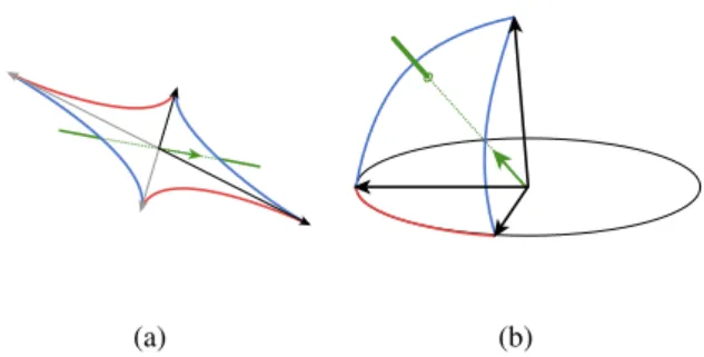
Figure 5: Adding sticks to the base glyphs to allow time-dependent glyphs to be represented. The eigen-vector ¯f corresponding to the time derivation is pro-jected onto the vectorg( ). A line cast from the center of the glyph in forward and backward direction ofg in-tersects the boundary of the glyph exactly twice, unless
gis the zero vector. Sticks ( ) representinggand -gare then added at those locations. (a) Construction of the 2D time-dependent Jacobian glyph. (b) Construction of one patch and one stick representing the eigenvalue ¯fof an 3D time-dependent Jacobian glyph.
whereaandbare the first two components of ¯f. This vector is then visualized by adding two identical sticks to the glyph, one representingg, the other −g
and both given a length ofs||g||, wheres>0∈Rcan
be used as a constant scaling factor. Rendering both ori-entations ofgis due to the fact, that ¯fis an eigenvector of ¯J, and therefore satisfies the same symmetry prop-erties. To reduce visual clutter, we move these sticks along the lines, given by their directions to the loca-tions where the line intersects the boundary of the un-derlying spatial glyph’s shape. Figure 5a illustrates this construction.
3.2
Time-Dependent 3D Tensor Glyphs
Finding new glyphs representing 3D time-dependent Jacobians is analogous to the 2D case. The addi-tional temporal information encoded by the Jacobian ¯
J∈R4×4is given by the additional eigenvector ¯f∈R4,
where ¯f= (a b c d)T.
We propose projecting ¯fonto the 3D vectorg∈R3by
using g = 1 ¯f a b c ,
and visualizing it by adding tubes to the spatial glyph, created by using eigenvalues and eigenvectors of J. These tubes are then moved along their vector direc-tions as well, until they reach the points, where their corresponding line would intersect the glyph patch. In that way, they are always visible and not rendered within the glyph, unless the temporal derivative is zero, in which case the new vector becomes the zero vector as demanded.
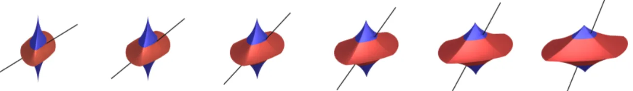
Figure 6: Glyphs representing different 2D Jacobians. The underlying features are less temporally stable to the left and more stable to the right. The stick has vanished in the last glyph, which shows that this feature is completely stable.
Figure 7: 3D Glyphs representing the same location in an unsteady flow field over time. The glyph as well as the stick representing the temporal derivative change smoothly over time.
Because both new constructions, 2D and 3D alike, fol-low the presented set of rules, they are suitable for cre-ating unique tensor glyphs for any given 2D or 3D Ja-cobian, unsteady or steady, and also follows all of the glyph design requirements that were discussed earlier.
4
RESULTS
First, we visualize different 2D time-dependent Ja-cobians. Figure 6 shows a selection of 2D glyphs for randomly chosen time-dependent 2D Jacobians with decreasing temporal derivative from left to right. These include glyphs based upon real-valued as well as complex-valued eigenvalues and eigenvectors. The additional sticks are always moved to the boundary of the spatial glyph, for any given shape.
In figures 9 and 10, our construction is applied to build glyphs representing the Jacobians at sampled locations of one time slice of a 2D unsteady flow behind a cylin-der. This is a sufficiently complex choice as a whole variety of different features is present as can be seen by the variety of different spatial glyphs. As the time pro-ceeds, alternating vortices, as illustrated by the glyphs using yellow and green colors, are created and trans-ported to the right. Therefore, Jacobians at several lo-cations comprise strong temporal derivatives, indicated by the additional sticks being clearly visible. Locations where the derivative vanishes are analogously indicated by small or even no sticks. While figure 9 shows the glyphs superimposed to an additional line integral con-volution (LIC) texture of the underlying flow field, fig-ure 10 displays the same glyphs in front of a different LIC texture which in this case represents the feature flow field[12] at the selected time. The projected ad-ditional eigenvectors are therefore tangent to this field at the given location. Two closeups for each field show zoomed-in areas of interest inside those fields.
To further highlight the sticks, the same domain is ren-dered without any supporting background LIC texture in figure 11.
Figure 7 demonstrates the new 3D glyphs, as it shows sampled time steps of the development of a 3D Jaco-bian at the same location evolved over time. The under-lying changing Jacobian is computed by linear interpo-lation of two vector field time slices. The spatial glyph changes independent of the time derivative, whereas the added tubes change direction due to the projected vec-tor, but change location due to change of glyph shape, as seen in figure 8.
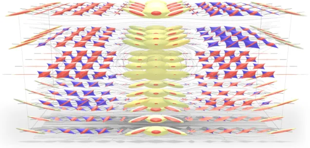
In figure 12, the glyphs are used to visualize regularly sampled locations in the 3D unsteady Jacobian field of an analytical flow with one moving center in the middle of the field. The whole flow is steadily moved to the right over time. To illustrate the underlying flow field, a set of illuminated streamlines is added. Here, too, the new glyphs show a variety of different underlying Jacobians, including constructions based upon tensors with complex and real-valued eigenvalues.
Figure 8: Sticks visualizing the temporal derivative are always moved along their directions to the boundary of the glyph, so they are always visible, no matter whether the spatial glyph is small (left) or large (right).
Figure 9: Glyphs visualizing the Jacobian matrix of the flow around a square cylinder with two closeups (rectan-gles). The underlying LIC image visualizes the fluid flow.
Figure 10: Glyphs visualizing the Jacobian matrix of the flow around a square cylinder with two closeups (rectan-gles). The underlying LIC image visualizes the feature flow.
Figure 11: Glyphs visualizing the Jacobian matrix of the flow around a square cylinder without additional sup-porting LIC textures.
5
DISCUSSION
Looking at figure 9, our newly designed 2D glyphs al-low to see the same structures of the underlying fal-low field as the steady or spatial 2D glyphs before. By find-ing a mappfind-ing onto the same visualization plane and moving it on the shape boundaries, encoding the addi-tional temporal information has not changed the spatial glyph. Therefore, rotational sections as well as laminar flows can still be easily determined in the given exam-ple flow. The same statement holds for the 3D case as displayed in figure 12. Even though, the addition of a
stick or tube respectively, is only a small extension to the known glyphs, it is one, that does not impair the expressiveness of the spatial glyph and offers a visu-alization technique for any 2D or 3D time-dependent Jacobian, symmetric or asymmetric.
As the sticks or tubes added to the glyphs are rendered in both directions of the vector, they not only follow the mathematical nature of eigenvector symmetry, they are also always visible, even in the 3D case, regardless of the point of view as long as the underlying Jacobian is unsteady. An appropriate scaling factor or a change of
Figure 12: 3D time-dependent flow with a moving vortex in the center. All features are moving to the right over time. The newly constructed glyphs are rendered at sampled locations at one time slice. Illuminated streamlines illustrate the underlying flow.
thickness can be chosen to further emphasize this addi-tion if necessary.
This work focuses on finding a construction of glyphs for general 2D and 3D time-dependent Jacobians while meeting a set of specific design requirements. The tran-sition between the different Jacobian glyphs is smooth, including a change of vector direction or vector length, which is displayed in figure 7, where a time series of the glyphs at the same location over time is shown. This al-lows our new construction method to seamlessly build upon the building requirements for the initial glyphs, and simply extend them.
When rendered on top of the feature flow field LIC tex-ture, as seen in figure 10, the glyph’s sticks are always tangent to it at the sampling location. This field allows tracking critical points over time (see, e.g., [12]) and therefore offers an insight of the progression of flow feature. We can predict glyphs with longer sticks to be moving or changing over time, while shorter or no sticks indicate that a feature is quite stable. The shown flow around the cylinder has vortices going along one axis to the right, which is also indicated by the sticks of the glyphs in those areas pointing in this direction. We can remove all supporting LIC textures as in figure 11 and still understand the flow itself, visualized by the spatial glyphs at the same time as the feature flow en-coded by the additional sticks. Inquiring the analytic flow shown in figure 12, all the glyphs indicate this be-havior by having tubes added to them, similar in length and direction, as the whole underlying flow is moving horizontally along one axis over time.
6
LIMITATION AND FUTURE WORK
Even though these extensions for the general second-order tensor glyphs can be applied to any temporal derivative of first-order tensor fields, this is not a con-struction method for general 4D second-order tensors. The fact, that the partial derivative of the added dimen-sion is always zero, allows us to utilize glyphs con-structed in the remaining subspaces. This added dimen-sion can then be projected onto the subspace and added to the glyph.
This work did not address deeper insights on visual per-ception of colors, controlled sampling of the underly-ing domain, or user studies, about the acceptance of the newly constructed glyphs. Dealing with cases of non-uniqueness when visualizing 3D tensors of rank 1 re-mains another inherited limitation of the glyph design based upon [3].
Our decision to move the sticks to the boundary of the glyph is mainly due to reducing visual clutter as well as to ensure visibility in the 3D case. However, in the 2D case, these sticks may give the impression to be only overlapped by the geometry and therefore be much longer, when the glyph is larger. As the two sticks rep-resent the symmetry property of an eigenvector, their directions are identical and only reflected. They cannot, however, provide any information about which choice of sign represents the actual change of position of the feature to the next time step.
7
REFERENCES
[1] Rita Borgo, Johannes Kehrer, David H Chung, Eamonn Maguire, Robert S Laramee, Helwig Hauser, Matthew Ward, and Min Chen. Glyph-based visualization: Foundations, design guide-lines, techniques and applications. Eurographics State of the Art Reports, pages 39–63, 2013. [2] G. Farin.Curves and Surfaces for CAGD. Morgan
Kaufmann, 5th edition, 2002.
[3] Tim Gerrits, Christian Rössl, and Holger Theisel. Glyphs for general second-order 2d and 3d ten-sors. IEEE Transactions on Visualization and Computer Graphics, 23(1):980–989, 2017. [4] Tobias Günther, Christian Rössl, and Holger
Theisel. Opacity optimization for 3d line fields.
ACM Trans. Graph., 32(4):120:1–120:8, July 2013.
[5] Marcel Hlawatsch, Philipp Leube, Wolfgang Nowak, and Daniel Weiskopf. Flow radar glyphs& static visualization of unsteady flow with uncertainty. Visualization and Computer Graph-ics, IEEE Transactions on, 17(12):1949–1958, 2011.
[6] A. Kratz, C. Auer, M. Stommel, and I. Hotz. Vi-sualization and analysis of second-order tensors: Moving beyond the symmetric positive-definite case. Computer Graphics Forum, 32(1):49–74, 2013.
[7] Robert S Laramee, Gordon Erlebacher, Christoph Garth, Tobias Schafhitzel, Holger Theisel, Xavier Tricoche, Tino Weinkauf, and Daniel Weiskopf. Applications of texture-based flow visualization.
Engineering Applications of Computational Fluid Mechanics, 2(3):264–274, 2008.
[8] Tony McLoughlin, Robert S Laramee, Ronald Peikert, Frits H Post, and Min Chen. Over two decades of integration-based, geometric flow vi-sualization. InComputer Graphics Forum, vol-ume 29, pages 1807–1829. Wiley Online Library, 2010.
[9] Armin Pobitzer, Ronald Peikert, Raphael Fuchs, Benjamin Schindler, Alexander Kuhn, Holger Theisel, Krešimir Matkovi´c, and Helwig Hauser. The state of the art in topology-based visualiza-tion of unsteady flow. InComputer Graphics Fo-rum, volume 30, pages 1789–1811. Wiley Online Library, 2011.
[10] Thomas Schultz and Gordon L Kindlmann. Su-perquadric glyphs for symmetric second-order tensors. Visualization and Computer Graphics, IEEE Transactions on, 16(6):1595–1604, 2010. [11] Nicholas Seltzer and Gordon Kindlmann. Glyphs
for Asymmetric Second-Order 2D Tensors. Com-puter Graphics Forum, 2016.
[12] H Theisel and HP Seidel. Feature flow field. In
Proceedings of the symposium on Data visualisa-tion, volume 2003, 2003.
[13] Markus Uffinger, Filip Sadlo, and Thomas Ertl. A time-dependent vector field topology based on streak surfaces. Visualization and Computer Graphics, IEEE Transactions on, 19(3):379–392, 2013.
[14] T. Weinkauf, H. Theisel, and O. Sorkine. Cusps of characteristic curves and intersection-aware visualization of path and streak lines. InProc. TopoInVis, April 2011.
[15] Tino Weinkauf, Jan Sahner, Holger Theisel, and Hans-Christian Hege. Cores of swirling parti-cle motion in unsteady flows. IEEE Transac-tions on Visualization and Computer Graphics, 13(6):1759–1766, 2007.