Accepted Manuscript
Looking-ahead in Backtracking Algorithms for Abstract Argumentation
Samer Nofal, Katie Atkinson, Paul E. Dunne
PII: S0888-613X(16)30118-9
DOI: http://dx.doi.org/10.1016/j.ijar.2016.07.013 Reference: IJA 7933
To appear in: International Journal of Approximate Reasoning Received date: 29 October 2015
Revised date: 25 July 2016 Accepted date: 26 July 2016
Please cite this article in press as: S. Nofal et al., Looking-ahead in Backtracking Algorithms for Abstract Argumentation,Int. J. Approx. Reason.(2016), http://dx.doi.org/10.1016/j.ijar.2016.07.013
This is a PDF file of an unedited manuscript that has been accepted for publication. As a service to our customers we are providing this early version of the manuscript. The manuscript will undergo copyediting, typesetting, and review of the resulting proof before it is published in its final form. Please note that during the production process errors may be discovered which could affect the content, and all legal disclaimers that apply to the journal pertain.
Looking-ahead in Backtracking Algorithms for Abstract
Argumentation
Samer Nofal
Computer Science Department, German Jordanian University, Jordan
Katie Atkinson, Paul E. Dunne
Computer Science Department, University of Liverpool, United Kingdom
Abstract
We refine implemented backtracking algorithms for a number of problems re-lated to Dung’s argumentation frameworks. Under admissible, preferred, com-plete, stable, semi stable, and ideal semantics we add enhancements, what are so-calledglobal looking-ahead pruning strategies, to the-state-of-the-art imple-mentations of two problems. First, we tackle the extension enumeration prob-lem: constructing some/all set(s) of acceptable arguments of a given argumenta-tion framework. Second, we address the acceptance decision problem: deciding whether an argument is in some/all set(s) of accepted arguments of a given argu-mentation framework. The experiments that we report show that the speedup gain of the new enhancements is quite significant.
Keywords: Algorithms, Argumentation Semantics, Argument-based reasoning
1. Introduction
Our study is centered around abstract argumentation frameworks (afs) in-troduced in [12]. afs are an important model for reasoning over conflicting ar-guments [17]. Applications ofafs are likely in diverse domains such as medicine [16], e-government [3] and agriculture [20]. Argumentation semantics are con-cerned with defining the acceptable arguments in a given af. There are a number of semantics for different motivations, see [2] for an excellent review. Several problems related to argumentation semantics are computationally hard [14]. In general, algorithms for solving these problems can be either direct or indirect; see the survey of [9]. Indirect approaches are reduction-based meth-ods such that the problem at hand is translated to another form to be solved by an off-the-shelf system. Direct approaches are dedicated algorithms (e.g. backtracking algorithms) that search for a solution to the input af. In this work we present improvements over the running-time efficiency of the state-of-the-art backtracking-based algorithms presented in [19, 18]. We highlight our contributions in two specific points:
1. Under a number of argumentation semantics (specified shortly) we en-hance the backtracking search (for sets of acceptable arguments) by a more powerful pruning strategy, so-called the global looking-ahead strat-egy.
2. We set out a backtracking-based approach to deciding acceptance under different semantics, i.e. whether an argument is in some/all set(s) of ac-ceptable arguments of a given af, without necessarily enumerating all such sets.
More concisely, we present an improved backtracking-based implementation for different problems in argumentation frameworks. The source code of the im-plementation is available athttp://sourceforge.net/projects/argtools/.
The main enhancement implemented is the global looking-ahead pruning strategy. Informally, this strategy enables a backtracking procedure (during traversing the search space) to regularly look-ahead for dead-ends (i.e. paths that do not lead to solutions) early enough such that considerable time is saved. Throughout the paper we precisely illustrate the new looking-ahead strategy. However, a high-level idea of the global looking-ahead is given in the next section after we present a necessary background on abstract argumentation frameworks. 2. Preliminaries
We recall the definition of abstract argumentation frameworks from [12]. Definition 1 (Dung’s Argumentation Frameworks). An abstract argumen-tation frameworkafis a pair(A, R)whereAis a set of abstract arguments and R⊆A×A is a binary relation, so-called the attack relation.
We refer to (x, y) ∈ R as x attacks y (or y is attacked by x). We denote by {x}− respectively{x}+ the subset ofAcontaining those arguments that attack (resp. are attacked by) the argumentx, and so we use{x}± to represent the set {x}+∪ {x}−; extending this notation in the natural way to sets of arguments, so that forS⊆A,
S− = { y∈A : ∃ x∈S s.t. y∈ {x}−} S+ = { y∈A : ∃ x∈S s.t. y∈ {x}+}
We say S ⊆ A attacks T ⊆ A (or T is attacked by S) if and only if
S+ ∩ T = ∅. S ⊆ A attacks x ∈ A (or x is attacked by S) if and only ifx∈S+. Given a subsetS ⊆A, then
• x∈ A is acceptable w.r.t. S if and only if for every (y, x) ∈ R, there is somez∈S for which (z, y)∈R.
• S isconflict free if and only if for each (x, y)∈S×S, (x, y)∈/R.
• Sisadmissibleif and only if it is conflict free and everyx∈Sis acceptable w.r.t.S.
• S is apreferred extension if and only if it is a⊆-maximal admissible set. • S is astable extension if and only if it is conflict free andS+=A\S.
• S is a complete extension if and only if it is an admissible set such that for each xacceptable w.r.t.S,x∈S.
• S is asemi stable extension if and only if it is admissible andS∪ S+ is maximal (w.r.t.⊆).
• Sis theideal extensionif and only if it is the maximal (w.r.t.⊆) admissible set that is contained in every preferred extension.
Preferred, complete and stable semantics are introduced in [12]. Ideal semantics is presented in [13] whereas semi stable semantics is presented in [24, 5]. Under these semantics, we are concerned with four problems:
P1. Given anafH = (A, R), enumerate all extensions ofH. P2. Given anafH = (A, R), build an extension ofH.
P3. Given an af H = (A, R) and an argument a ∈ A, decide whether a
is in some extension of H. In the literature this is called the credulous acceptance problem.
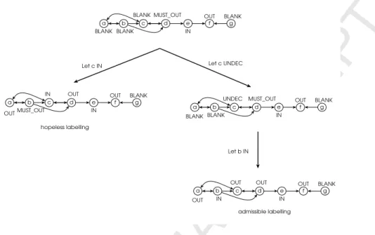
P4. Given anafH = (A, R) and an argument a∈A, decide whetherais in all extensions ofH. This is called theskeptical acceptance problem. To provide an overview of the new looking-ahead strategy consider for ex-ample theaf depicted in figure 1. Assume a backtracking procedure tries to build a preferred extension starting with the set S = {b}. Then, assume the procedure adds the argument e to S. At this point, our new global looking-ahead will detect thatS is not possible to be expanded to a preferred extension becausebcan not be defended anymore; so the procedure will not try to extend further any setT ⊇ {b, e}, whereas previous backtracking algorithms may not discover such conflict in an early stage of the search process. Global looking-ahead is a simple yet powerful mechanism. In the following sections we explain how to incorporate the global looking-ahead in the state-of-the-art backtrack-ing algorithms in a cost-effective way such that the overall performance of the algorithms is significantly improved.
The rest of the paper is structured as follows, in section 3 we present the algorithms for problems P1 & P2 along with a demonstration on the new en-hancement. Then in section 4 we give the algorithms for problems P3 & P4 with the new features explained. In section 5 we show experimentally how the refined algorithms result in a better performance, and lastly we conclude the paper in section 6.
Figure 1: A backtracking procedure using the new looking-ahead will not try anyT ⊇ {b, e}.
3. Enhanced looking-ahead in backtracking algorithms for the exten-sion enumeration problem
We present respectively enhanced algorithms for listing preferred extensions, admissible sets, complete extensions, stable extensions, semi stable extensions, and lastly for constructing the ideal extension.
3.1. Preferred Semantics
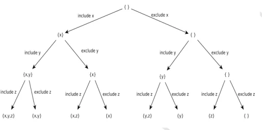
Before presenting our algorithm in full, we give the reader a high-level notion of backtracking algorithms. As we are concerned with building extensions (i.e. subsets of arguments) consider the task of subset enumeration ofA={x, y, z}. Then, a backtracking search procedurerecursively traverses a conceptual binary tree in which the root node is an empty set{}. Then the procedure forks to a left (respectively right) node by including (respectively excluding) some argument, sayx. Thus, the left subtree represents all possible subsetsS⊇ {x}, whereas the right subtree represents all possible subsets T {x}. See figure 2 that shows an implicit binary tree for a backtracking procedure constructing subsets of {x, y, z}. As the problems we tackle in this paper are in general around building set-inclusion maximal subsets then all of the algorithms of the paper traverse the binary tree (see figure 2) from left to right to make sure that maximal sets are visited first, and so maximality check is made more efficient. Referring to figure 2, to check whether{x}is a subset of other solution subsets all we need is to compare {x} with the constructed subsets so far. This is true because the subsets not constructed yet certainly do not include {x}. Concluding a general description of the backtracking search, we note that a search procedure backtracks and follows a different path if it detects that a solution can not be reached by pursuing the current path. Or the procedure simply backtracks to find another solution.
So far, we discussed argumentation semantics using set-theoretic notations to define different kind of extensions. Another way to define argumentation seman-tics is in terms oflabellings. A common comprehensive handling of labelling-based semantics is introduced in [6], where it is shown that extensions and
labellingsare interchangeable. In [6] argumentation semantics are characterized using three-label mappingλ→ {IN, OU T, U N DEC}. For example let (A, R) be anaf and S ⊂A be an admissible set, then the corresponding admissible labellingλ→ {IN, OU T, U N DEC}forS is defined by the set
Figure 2: subset enumeration of the set{x, y, z}.
{(x, IN)|x∈S} ∪ {(x, OU T)|x∈S+} ∪ {(x, U N DEC)|x∈A\(S∪S+)}. In other words the IN label denotes that an argument is in the setS ⊂A, the OUT label that an argument is attacked byS and the UNDEC label that none of the previous holds.
For the purpose of constructing argument extensions, we use a five-label mappingLab:A→ {IN, OU T, U N DEC, BLAN K, M U ST OU T}. The extra labels, BLANK & MUST OUT, are used for algorithmic purposes only. The BLANK label is the initial label for all arguments in a givenaf. An argument
xis labeled with MUST OUT if and only if:
1. there is an argumenty withLab(y) =IN such thatx∈ {y}−, 2. and there is no argumentz withLab(z) =IN such thatx∈ {z}+. The MUST OUT label denotes an argument that must be labeled OUT to make the set of IN arguments admissible, but does not have yet an attacker labeled IN. Our algorithm is a depth-first-search backtracking procedure (and so all of the algorithms presented in the paper) that passes along an abstract binary tree. The nodes of the tree are different states of a total mappingLab:
A→ {IN, OU T, U N DEC, BLAN K, M U ST OU T}. In what follows we define different kinds of states, from now on we refer to these states by labellings. We start with defining the initial labelling (i.e. the root node of the binary tree.) Definition 2 (Initial Labelling). LetH = (A, R)be anafandS ⊆Abe the set of self-attacking arguments. Then the initial labelling ofH is defined by the union: {(x, BLAN K)|x∈A\S} ∪ {(y, U N DEC)|y∈S}.
Trying to build a set including (respectively excluding) some argument, the algorithm forks to a left (respectively right) node by what we calltransitions.
Recall that we build conflict-free sets, and so including an argument in a set will consequently expel the neighbor arguments out of the set. Hence, a left-transitioninvolves three actions: labelling some argument with IN, its attackers with MUST OUT while the arguments it attacks are labeled OUT. A right-transition is basically equivalent to labelling some argument with UNDEC. In what follows we precisely define left and right transitions.
Definition 3 (Left-Transition). Let H = (A, R)be an af,Lab:A→ {IN, OU T, U N DEC, M U ST OU T, BLAN K} be a total mapping andxbe an argu-ment withLab(x) =BLAN K. Then the left-transition ofLabto a new labelling Lab usingxis defined by:
1. Lab ←Lab.
2. Lab(x)←IN.
3. for eachy ∈ {x}+, Lab(y)←OU T.
4. for each z∈ {x}− with Lab(z)=OU T, Lab(z)←M U ST OU T.
Definition 4 (Right-Transition). LetH = (A, R)be anaf,Lab:A→ {IN, OU T, U N DEC, M U ST OU T, BLAN K} be a total mapping and x be an ar-gument with Lab(x) = BLAN K. Then the right-transition of Lab to a new labellingLab usingxis defined by:
1. Lab ←Lab.
2. Lab(x)←U N DEC.
We specify terminal labellings that are associated with leaf nodes of the search tree. Terminal labellings imply that further transitions are not possible simply because there is no argument left with the BLANK label.
Definition 5 (Terminal Labellings). Let H = (A, R) be an af and Lab :
A→ {IN, OU T, U N DEC, M U ST OU T, BLAN K} be a total mapping. Then Lab is a terminal labelling of H if and only if for each x ∈ A, Lab(x) =
BLAN K.
Terminal labellings are either dead ends or solutions. Here we define dead-end labellings.
Definition 6 (Dead-end Labellings). Let H = (A, R) be an af and Lab :
A→ {IN, OU T, U N DEC, M U ST OU T, BLAN K} be a total mapping. Then Lab is a dead-end labelling of H if and only if Lab is a terminal labelling and there isx∈A with Lab(x) =M U ST OU T.
Now we define solution states. A solution state is actually a labelling that corresponds to a preferred extension. We define firstadmissible labellings then
preferred labellings.
Definition 7 (Admissible Labellings). Let H = (A, R)be anaf andLab:
A→ {IN, OU T, U N DEC, M U ST OU T, BLAN K} be a total mapping. Then Lab is an admissible labelling ofH if and only if Lab is terminal and there is noxwithLab(x) =M U ST OU T.
Definition 8 (Preferred Labellings). Let H = (A, R) be an af and Lab :
A→ {IN, OU T, U N DEC, M U ST OU T, BLAN K} be a total mapping. Then Labis a preferred labelling ofH if and only ifLabis an admissible labelling and
{x|Lab(x) =IN} is maximal (w.r.t. ⊆) among all admissible labellings.
We give now algorithm 1 that finds all preferred extensions of a given af when called with the initial labelling. This is to show a high-level view of the basic mechanism of all algorithms presented in the paper. Note that all procedures in this paper are called by reference to the passed parameters, unless otherwise specified.
Algorithm 1:Enumerate Preferred(H, Lab, E) input :H is anaf,
Lab:A→ {IN, OU T, U N DEC, M U ST OU T, BLAN K},
E⊆2A.
output:Lab:A→ {IN, OU T, U N DEC, M U ST OU T, BLAN K},
E⊆2A.
1 if Lab is a dead-end labelling then
2 return;
3 if Lab is a terminal labelling then 4 if Lab is an admissible labelling then
5 if {x|Lab(x) =IN} is not a subset of any set inE then
6 E←E∪ {{x|Lab(x) =IN}};
7 return;
8 select any argumentxwith Lab(x) =BLAN K;
9 get a new labellingLab by applying the left-transition ofLabusingx; 10 call Enumerate Preferred(H, Lab, E);
11 get a new labellingLab by applying the right-transition ofLabusingx; 12 call Enumerate Preferred(H, Lab, E);
The behavior of algorithm 1 is depicted in figure 3. We illustrate that algorithm 1 is sound and complete.
Proposition 1. Let H= (A, R)be anaf,Lab be the initial labelling ofH and E=∅. Then after calling algorithm 1 withEnumerate P ref erred(H, Lab, E), E is the set of all preferred extensions ofH.
Proof: Algorithm 1, and so all of the algorithms of the current paper, can be proved by contradiction. Firstly we note that completeness is guaranteed by the fact that the algorithm builds every conflict-free subset ofA, which follows directly from definitions 3 & 4. Also note that conflict-free sets are added to the setE if and only if they are admissible and not a subset of any admissible set inE. To show the soundness, assume that algorithm 1 reported incorrectly
S preferred. Then, S is not a maximal (w.r.t. ⊆) admissible set. S being not admissible is a contradiction with the actions of line 4 of the algorithm. IfS
is admissible but not maximal then there is a preferred extensionT ∈E such that S ⊆T. This contradicts with the actions of line 5 together with the fact
that maximal subsets are constructed first. I
Note that algorithm 1 backtracks if a dead-end labelling is reached or it backtracks to find another preferred extension. To improve the performance of algorithm 1 we note dead-end labellings can be detected earlier before reaching them. Therefore, we define ahopeless labelling, expanding of which will lead only to dead-end labellings.
Definition 9 (Hopless Labelling). Let H = (A, R)be anafandLab:A→
{IN, OU T, U N DEC, M U ST OU T, BLAN K} be a total mapping. Then Lab is a hopeless labelling of H if and only if there is x ∈ A with Lab(x) =
M U ST OU Tsuch that for ally∈ {x}−Lab(y)∈ {OU T, M U ST OU T, U N DEC}.
We give algorithm 2 that backtracks whenever a hopeless labelling is reached. This mechanism, i.e. detecting (and avoiding) fruitless paths before getting to a dead-end labelling, is the spirit of the newlooking-ahead enhancements.
Algorithm 2:Enumerate Preferred(H, Lab, E) input :H is anaf,
Lab:A→ {IN, OU T, U N DEC, M U ST OU T, BLAN K},
E⊆2A.
output:Lab:A→ {IN, OU T, U N DEC, M U ST OU T, BLAN K},
E⊆2A.
1 if Labis a hopeless labelling thenreturn; 2 if Lab is a terminal labelling then 3 if Lab is an admissible labelling then
4 if {x|Lab(x) =IN} is not a subset of any set inE then
5 E←E∪ {{x|Lab(x) =IN}};
6 return;
7 select any argumentxwith Lab(x) =BLAN K;
8 get a new labellingLab by applying the left-transition ofLabusingx; 9 call Enumerate Preferred(H, Lab, E);
10 get a new labellingLab by applying the right-transition ofLabusingx; 11 call Enumerate Preferred(H, Lab, E);
We illustrate the soundness and completeness of algorithm 2.
Proposition 2. Let H= (A, R)be anaf,Lab be the initial labelling ofH and E=∅. Then after calling algorithm 2 withEnumerate P ref erred(H, Lab, E), E is the set of all preferred extensions ofH.
Proof: It follows directly from the similarity between algorithm 2 and al-gorithm 1. The only difference between alal-gorithm 1 and alal-gorithm 2 is that algorithm 1 backtracks if a dead-end labelling is reached while algorithm 2
instead backtracks if a hopeless labelling is reached. Recall that a dead-end labelling is a terminal labelling in contrary to a hopeless labelling, which is not necessarily terminal. However, if we further expand a hopeless labelling, then by its definition we ended up with a dead-end labelling. Note that a labellingLab
being hopeless implies the fact that there isxwithLab(x) =M U ST OU T such that for ally ∈ {x}− Lab(y)∈ {OU T, M U ST OU T, U N DEC}. Transitioning suchLabwill not change this situation, which is a basic condition of dead-end
labellings. I
We add now two changes to algorithm 2 that also improve the efficiency of preferred extension enumeration. The first change is about the argument selection for labelling transition. In all of the presented algorithms we select an argumentxwith Lab(x) =BLAN K such thatxhas the maximum number of neighbors, we call suchxaninfluential argument.
Definition 10 (Influential Arguments). Let H = (A, R) be an af, x∈ A andLab :A→ {IN, OU T, U N DEC, M U ST OU T, BLAN K} be a total map-ping. Thenxis influential if and only ifLab(x) =BLAN K and for ally with Lab(y) =BLAN K |{x}±| ≥ |{y}±|.
For the second change of algorithm 2 we note BLANK arguments that are attacked only by OUT/MUST OUT arguments must be labeled IN because if the current labelling expanded to an admissible labelling then these arguments will be acceptable with respect to the constructed admissible set. Thus, we prop-agate labellings usingmust-in arguments. A definition ofmust-in arguments is given first then followed by a specification for labellingpropagation.
Definition 11 (Must-in Arguments). Let H = (A, R) be an af, x ∈ A andLab :A→ {IN, OU T, U N DEC, M U ST OU T, BLAN K} be a total map-ping. Then x is must-in if and only if Lab(x) = BLAN K and for all y ∈
{x}− Lab(y)∈ {OU T, M U ST OU T}.
Definition 12 (Labelling Propagation). LetH = (A, R)be anafandLab:
A→ {IN, OU T, U N DEC, M U ST OU T, BLAN K} be a total mapping. Then the propagation ofLab is defined by the following actions:
1. if there is no must-in argument, then halt.
2. pick a must-in argumentx.
3. Lab(x)←IN.
4. for each y∈ {x}+, Lab(y)←OU T.
5. go to 1.
Now, we present algorithm 3 that includes the two changes, i.e. argument selection and labelling propagation. The changes implemented in lines 8 & 9.
Here we illustrate that algorithm 3 is sound and complete.
Proposition 3. Let H = (A, R)be anaf,Labbe the initial labelling ofH and E=∅. Then after calling algorithm 3 withEnumerate P ref erred(H, Lab, E), E is the set of all preferred extensions ofH.
Algorithm 3:Enumerate Preferred(H, Lab, E) input :H is anaf,
Lab:A→ {IN, OU T, U N DEC, M U ST OU T, BLAN K},
E⊆2A.
output:Lab:A→ {IN, OU T, U N DEC, M U ST OU T, BLAN K},
E⊆2A.
1 if Lab is a hopeless labelling then
2 return;
3 if Lab is a terminal labelling then 4 if Lab is an admissible labelling then
5 if {x|Lab(x) =IN} is not a subset of any set inE then
6 E←E∪ {{x|Lab(x) =IN}};
7 return;
8 propagateLab;
9 select anyx∈Asuch thatxis influential;
10 get a new labellingLab by applying the left-transition ofLabusingx; 11 call Enumerate Preferred(H, Lab, E);
12 get a new labellingLab by applying the right-transition ofLabusingx; 13 call Enumerate Preferred(H, Lab, E);
Proof: Algorithm 3 differs from algorithm 2 in two issues: argument selection (line 9) and labelling propagation (line 8). We note that any argument selec-tion strategy is valid and does not affect the soundness/completeness of the algorithm. As to the labelling propagation soundness, assume the algorithm reported incorrectly S admissible due to an argument x ∈ S that was incor-rectly added by labelling propagation. This means x is not acceptable to S, and hence there isy∈ {x}− with Lab(y) =U N DEC. This is a contradiction, recall labelling propagation is about including arguments that are attacked only by OUT/MUST OUT arguments. Lastly, observe that by labelling propagation we exclude admissible labellings that are not preferred due to the existence of
must-in arguments; hence the algorithm is complete. I
We present now algorithm 4, an optimized version of algorithm 3. There are three optimization points. For the first point, we drop the recursive call after a right-transition and put a while structure to do the required loop operation, see lines 3 & 7. For the second optimization point, we increase the number of checks for a hopeless labelling. Now we check for a hopeless labelling every time a labelling changes. Thereby we possibly save a considerable amount of running-time, see lines 2 & 6 & 8. For the third optimization, we start the algorithm by propagating labellings. Consider for example an acyclic inputaf, then by applying labeling propagation only we get the preferred extension of the givenaf.
Algorithm 4:Enumerate Preferred(H, Lab, E) input :H is anaf,
Lab:A→ {IN, OU T, U N DEC, M U ST OU T, BLAN K},
E⊆2A.
output:Lab:A→ {IN, OU T, U N DEC, M U ST OU T, BLAN K},
E⊆2A. 1 propagateLab;
2 if Labis hopelessthenreturn; 3 whileLab is not terminaldo
4 select anyx∈Asuch that xis influential;
5 get a new labelling Lab by running the left-transition of Labusing x; 6 if Lab is not hopelessthenEnumerate Preferred(H, Lab, E); 7 update Labby applying the right-transition ofLab usingx; 8 if Lab is hopelessthenreturn;
9 if Lab is admissible then
10 if {x|Lab(x) =IN} is not a susbet of any set ofE then 11 E←E∪ {{x|Lab(x) =IN}};
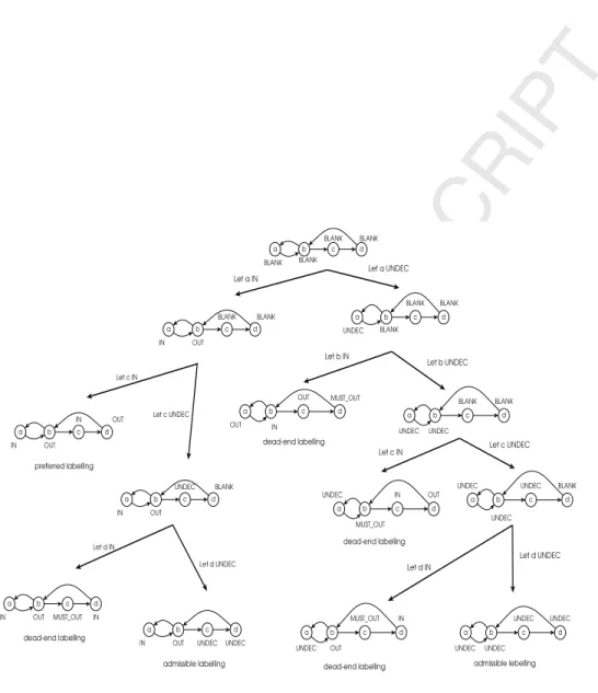
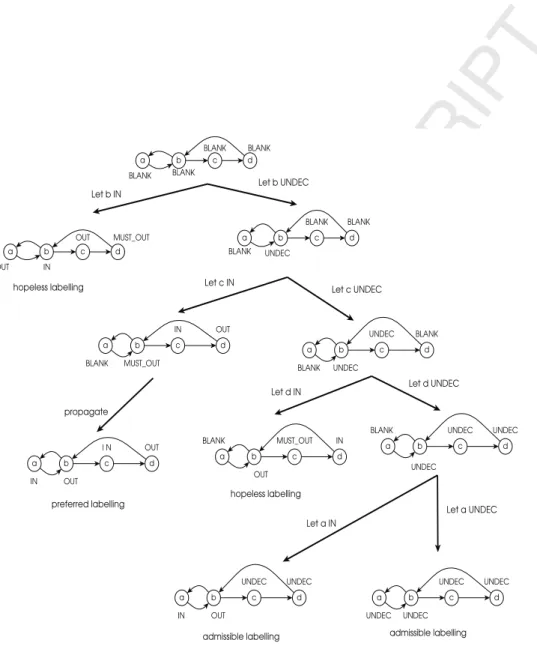
completeness) of our algorithm. Figure 4 depicts the behavior of algorithm 4 in listing the preferred extensions of a givenaf. We do not mean by this example to show the improvements brought by algorithm 4. In fact, the algorithm of [19] will behave on this example similarly to algorithm 4.
Now we show the improvement of algorithm 4 over the algorithm of [19]. To do so, we recall the hopeless labelling characterization of [19].
Definition 13 (Hopeless Labellings of [19]). Let H = (A, R) be an af, x∈AandLab:A→ {IN, OU T, U N DEC, M U ST OU T, BLAN K} be a total mapping such thatLab(x) =IN. ThenLab is a hopeless labelling ofH due to xif and only if there is y∈ {x}− with Lab(y) =M U ST OU T such that for all z∈ {y}− Lab(z)∈ {OU T, M U ST OU T, U N DEC}.
Now we are ready to give the two differences between algorithm 4 and the algorithm of [19]:
Diff 1. The algorithm of [19] identifies hopeless labellings by checking the at-tackers of some argument (that is why we call it a local looking-ahead), whereas algorithm 4 captures hopeless labellings by investigating every argument with the label MUST OUT in the framework (that is why we call it aglobal looking-ahead).
Diff 2. The algorithm of [19] checks for hopeless labellings less often, only after left-transitions. In contrast, algorithm 4 checks for hopeless labellings on three occasions, see lines 2, 6 & 8.
We present an example to show the impact of the new enhancement. Refer-ring to figure 5, at this state of the given af algorithm 4 stops searching and
Figure 5: An example to show the enhancement of algorithm 4 over the state-of-the-art algorithm presented in [19].
backtracks because the argumenta, which is labelled MUST OUT, is attacked only by the argumentf that is OUT. On the contrary, the algorithm of [19] will continue searching by testing the argumentgwith the label IN, which is unpro-ductive. However, we verify experimentally the significance of the enhancement in section 5.
3.2. Admissible Sets
For listing admissible sets we present algorithm 5, which is a modification of algorithm 4. There are two differences between algorithm 4 and algorithm 5: Diff 1. Labelling propagation is not applicable for enumerating admissible sets. Diff 2. By definition, maximality check is not needed for building admissible sets.
To justify Diff 1, consider an af H = ({a, b, c},{(a, b),(b, c)}) withLab = {(a, IN),(b, OU T),(c, BLAN K)}. Then, using the argument c algorithm 5
performs a left-transition and then a right-transition to report respectively {a, c} and {a} admissible. In contrast, algorithm 4 will propagate Lab to {(a, IN),(b, OU T),(c, IN)}, thereby building the preferred extension {a, c}. Note that with labelling propagation the admissible set{a} is overlooked.
Algorithm 5:Enumerate Admissible(H, Lab, E) input :H is anaf,
Lab:A→ {IN, OU T, U N DEC, M U ST OU T, BLAN K},
E⊆2A.
output:Lab:A→ {IN, OU T, U N DEC, M U ST OU T, BLAN K},
E⊆2A.
1 whileLab is not terminaldo
2 select anyx∈Asuch that xis influential;
3 get a new labelling Lab by running the left-transition of Labusing x; 4 if Lab is not hopelessthenEnumerate Admissible(H, Lab, E); 5 update Labby applying the right-transition ofLab usingx; 6 if Lab is hopelessthenreturn;
7 if Lab is admissible then
8 E ←E∪ {{x|Lab(x) =IN}};
3.3. Complete Semantics
To present our algorithm for complete extension enumeration, we define first complete labellings.
Definition 14 (Complete Labellings). Let H = (A, R)be an af andLab:
A→ {IN, OU T, U N DEC, M U ST OU T, BLAN K} be a total mapping. Then Labis a complete labelling of H if and only ifLab is admissible and for each x withLab(x) =U N DEC there isy∈ {x}− with Lab(y) =U N DEC.
Thus, complete labellings go hand in hand with labelling propagation. This is because a complete labelling can not be reached if a procedure applies a right-transition using a must-in argument, which is a BLANK argument that is attacked only by OUT/MUST OUT arguments. Next we prove that a complete labelling corresponds to a complete extension, i.e. the set of IN arguments of a given complete labelling is a complete extension.
Proposition 4. Let H = (A, R) be an af and Lab be a complete labelling of H. Then, the setS ={x|Lab(x) =IN} is a complete extension ofH.
Proof: Assume S is admissible but not complete. Then there is x∈ S with
Lab(x) = U N DEC such that x is acceptable to S. This is in contradiction to the definition of complete labellings. Similarly, S being not admissible is a
contradiction. I
Consider anafH = ({a, b, c},{(a, b),(b, a),(b, c),(c, b)}) withLab={(a, U N DEC),(b, OU T),(c, IN)}. Then, {c} is admissible but not complete be-causea, which is withLab(a) =U N DEC, is acceptable w.r.t.{c}. Therefore, algorithm 6 differs from algorithm 4 in two aspects:
1. Maximality check is not required for listing complete extensions, contrary to preferred extensions.
2. By the definition of complete labellings, the property that every UNDEC argument being attacked by an UNDEC argument is essential in identify-ing complete extensions, see line 9 of algorithm 6.
Algorithm 6:Enumerate Complete(H, Lab, E) input :H is anaf,
Lab:A→ {IN, OU T, U N DEC, M U ST OU T, BLAN K},
E⊆2A.
output:Lab:A→ {IN, OU T, U N DEC, M U ST OU T, BLAN K},
E⊆2A. 1 propagateLab;
2 if Labis hopelessthenreturn; 3 whileLab is not terminaldo
4 select anyx∈Asuch that xis influential;
5 get a new labelling Lab by running the left-transition of Labusing x; 6 if Lab is not hopelessthenEnumerate Complete(H, Lab, E); 7 update Labby applying the right-transition ofLab usingx; 8 if Lab is hopelessthenreturn;
9 if Lab is a complete labellingthen 10 E ←E∪ {{x|Lab(x) =IN}};
3.4. Stable Semantics
Recall that ifS is a stable extension of anafH = (A, R) thenS+ =A\S. Therefore the UNDEC label is not usable in characterizing stable semantics, and so stable extensions can be constructed by using a 4-label mappingLab :
A → {IN, OU T, M U ST OU T, BLAN K}. Although left-transitions are valid for listing stable extensions, we note right-transitions are not applicable any more due to the absence of the UNDEC label. In the following definition we describe right-transitions for listing stable extensions.
Definition 15 (Right-Transition-Stable). Let H = (A, R)be an af, Lab:
A→ {IN, OU T, M U ST OU T, BLAN K} be a total mapping andxbe an argu-ment withLab(x) =BLAN K. Then the right-transition-stable of Labto a new labellingLab usingxis defined by:
1. Lab ←Lab.
We emphasize that for listing stable extensions we use a 4-label mapping instead of a 5-label mapping in specifying the initial labelling, left transitions, terminal labellings, dead-end labellings, hopeless labellings, must-in arguments, labelling propagation, and influential arguments. These concepts are analogous to the ones under preferred semantics but again with dropping the UNDEC label. Now we describe stable labellings.
Definition 16 (Stable Labellings). LetH= (A, R)be anafandLab:A→
{IN, OU T, BLAN K, M U ST OU T} be a total mapping. Then Lab is a stable labelling of H if and only ifLab is terminal and there is no x with Lab(x) =
M U ST OU T.
Observe that stable labellings capture stable extensions. LetH= (A, R) be an af and Lab be a stable labelling of H. Then it follows directly, from the definition of stable labellings and right-transition-stable, that the setS ={x| Lab(x) =IN}is a stable extension ofH.
For listing stable extensions, we present algorithm 7. Algorithm 7:Enumerate Stable(H, Lab, E)
input :H is anaf,
Lab:A→ {IN, OU T, M U ST OU T, BLAN K},
E⊆2A.
output:Lab:A→ {IN, OU T, M U ST OU T, BLAN K},
E⊆2A. 1 propagateLab;
2 if Labis hopelessthenreturn; 3 whileLab is not terminaldo
4 select anyx∈Asuch that xis influential;
5 get a new Lab by running the left-transition of Labusingx; 6 if Lab is not hopelessthenEnumerate Stable(H, Lab, E); 7 update Labby applying the right-transition-stable ofLab usingx; 8 if Lab is hopelessthenreturn;
9 if Lab is a stable labelling then 10 E ←E∪ {{x|Lab(x) =IN}};
To summarize, algorithm 7 is different from algorithm 4 in three issues: 1. By definition, maximality check is not required for listing stable
exten-sions.
2. Algorithm 7 uses a four-label mapping
Lab:A→ {IN, OU T, M U ST OU T, BLAN K},
whereas algortihm 4 applies a five-label mapping
Lab:A→ {IN, OU T, M U ST OU T, U N DEC, BLAN K}.
3. The right-transitions for stable extension enumeration is modified as spec-ified in definition 15.
3.5. Semi Stable Semantics
For listing semi stable extensions we present algorithm 8. It is known that a subset S is semi stable if it is preferred and S∪S+ is maximal among all preferred extensions (see [2]). Thus, algorithm 8 performs additional steps (on top of what algorithm 4 does) to find semi stable extensions from the constructed set of all preferred extensions, see lines 1 - 3 of algorithm 8. Consider an af
H= ({a, b, c},{(a, b),(b, a),(b, c),(c, c)}) then there are two preferred extensions {a}&{b}while there is only one semi stable extension, which is{b}.
Algorithm 8:Enumerate Semi Stable(H, Eprf, E) input :H is anaf,
Eprf is the set of the preferred extensions ofH,
E⊆2A. output:E⊆2A. 1 foreachS∈Eprf do 2 if T ∈Eprf with S∪S+T∪T+ then 3 E←E∪ {S}; 3.6. Ideal Semantics
Now we present algorithm 9 for constructing the ideal extension. Note that the ideal extension is the maximal complete extension that is not attacked by any other complete extension, see [2]. Therefore, algorithm 9 builds the ideal extension by firstly constructing all complete extensions. Then it picks the ideal extension from the listed complete extensions, see lines 1- 4. Observe that all algorithms in this paper are designed to enumerate extensions in descending order (w.r.t. ⊆) from a maximal extension to a minimal one; hence at line 1 there is no extra work to be done to traverse complete extensions in this order.
Algorithm 9:Build The Ideal Extension(H, Ecom) input :H is anaf,
Ecomis the set of the complete extensions ofH.
1 foreachS∈Ecom do// descendingly w.r.t. set inclusion 2 if ∀T ∈EcomT+∩S=∅then
3 reportS is the ideal extension;
4 halt;
4. Enhanced backtracking algorithms for the acceptance problem We present algorithms for deciding credulous and skeptical acceptance prob-lem under preferred and stable semantics.
4.1. Credulous acceptance under preferred, complete and admissible semantics
It is known that an argument is credulously accepted under preferred, ad-missible and complete semantics if and only if the argument is in an adad-missible set. Since we are concerned with deciding an acceptance of some argument, sayx, then the first step is to label xwith IN and next to apply the effect on the neighbor arguments. We define the initial labelling for deciding credulous acceptance.
Definition 17 (Initial Labelling for Deciding Acceptance). LetH = (A, R)
be anaf,xbe an argument, S⊆A be the set of self-attacking arguments such that x∈S. Then, the initial labelling of H for deciding an acceptance of xis defined by the union of the sets:
{(x, IN)} ∪
{(y, OU T)|y∈ {x}+} ∪
{(z, M U ST OU T)|z∈ {x}−} ∪
{(v, BLAN K)|v∈S∪ {x}±∪ {x}} ∪
{(u, U N DEC)|u∈S\ {x}±}.
We note a terminal labeling, as defined earlier, is no more applicable to deciding credulous acceptance. This is because a credulous acceptance of some argument is affected bysome(i.e. not all) of the BLANK arguments, which are those that have a directed path to the argument in question. For example in figure 6 the argumentg has no effect on the credulous acceptance status of the argumente. We give below a new definition for terminal labellings.
Definition 18 (Terminal Labellings for Deciding Acceptance). LetH =
(A, R)be anaf,xbe an argument andLab:A→ {IN, OU T, U N DEC, M U ST OU T, BLAN K} be a total mapping. Then Lab is a terminal labelling of H for deciding an
ac-ceptance of xif and only if there is no(y, z)∈R with Lab(y) =BLAN K and Lab(z) =M U ST OU T.
Another issue with deciding credulous acceptance is the concept of influential arguments. Earlier we call an argument influential if it is labelled BLANK and has the maximum number of neighbors among all BLANK arguments. Again, deciding acceptance (for a given argument) is only affected by the arguments that have a directed path to the argument in question. So, we are interested in the influential arguments that have a directed path to the argument in ques-tion. We modify the definition of influential arguments for deciding credulous acceptance.
Definition 19 (Influential Arguments for Deciding Acceptance). LetH =
(A, R)be anaf,xbe an argument,Lab:A→ {IN, OU T, U N DEC, M U ST OU T, BLAN K} be a total mapping,Q={u with Lab(u) =BLAN K| there is v∈ {u}+with Lab(v) = M U ST OU T} andy∈Q. Then,y is influential in deciding a credulous accep-tance ofxif and only if for all z∈Q|{y}±| ≥ |{z}±|.
Figure 6: How algorithm 10 decides a credulous acceptance ofein a givenaf.
We present algorithm 10 for deciding credulous acceptance, see figure 6 that shows how algorithm 10 works.
We summarize now the differences between algorithm 10 and algorithm 4: 1. Maximality check is not required for deciding credulous acceptance, recall
algorithm 10 basically builds an admissible set containing the argument in question.
2. The initial labelling is different, see definition 17. 3. Terminal labellings are different, see definition 18. 4. Influential arguments are different, see definition 19.
It is not hard to see the soundness and completeness of algorithm 10. Proposition 5. LetH = (A, R)be anaf,xbe an argument andLabis the ini-tial labelling ofH for deciding a credulous acceptance ofx. Then algorithm 10, by calling Decide Credulous(H,x,Lab), decides a credulous acceptance ofx.
Proof: Directly from similar structure of algorithm 10 and algorithm 4. I Now we compare algorithm 10 with the algorithm of [19] for deciding cred-ulous acceptance; there are three differences:
1. The first difference is stylistic only. In [19] the algorithm uses the labeling
Lab:A→ {P RO, OP P, OU T, M U ST OU T, U N DEC, BLAN K}
while algorithm 10 uses
Algorithm 10:Decide Preferred Credulous(H, x, Lab) input :H is anaf,
xis the argument in question,
Lab:A→ {IN, OU T, U N DEC, BLAN K, M U ST OU T}. output:Lab:A→ {IN, OU T, U N DEC, BLAN K, M U ST OU T}. 1 propagateLab;
2 if Labis hopelessthenxis not accepted, halt; 3 whileLab is not terminaldo
4 select anyx∈Asuch that xis influential;
5 get a new labelling Lab by running the left-transition of Labusing x; 6 if Lab is not hopelessthenDecide Credulous(H, x, Lab);
7 update Labby applying the right-transition ofLab usingx; 8 if Lab is hopelessthenreturn;
9 if Lab is admissible then
10 report xis accepted,xis in the admissible set{y|Lab(y) =IN};
11 halt;
The PRO label is applied in the same way the IN label is used in al-gorithm 10. The actual difference between the two mappings is the use of the OPP label. For a built admissible set S, an argument x with
Lab(x) =OP P implies thatx∈S+∩S− whereas in algorithm 10 such
xis mapped to OUT. Note that in [19] the concern was to compare with related work that uses PRO & OPP. In this paper we opt to keep labeling mappings consistent in all algorithms for readability. Again, we stress that this issue (i.e. which of the two mappings to use) is a choice matter that has negligible effect on running-time efficiency.
2. Algorithm 10 applies labelling propagation. This is not the case in the algorithm of [19].
3. Lastly we note that algorithm 10 is enhanced in the same way algorithm 4 is improved over the algorithm of [19] for preferred extension enumeration, see subsection 3.1.
4.2. Deciding skeptical acceptance under preferred semantics
We present algorithm 11 for deciding skeptical acceptance. The algorithm tries to buildall preferred extensions that include the argument in question; if no preferred extension is found then the argument is not skeptically accepted. Otherwise, the algorithm tries to build one preferred extension without the concerned argument. If such extension is not found then the algorithm concludes that the argument is accepted. If the algorithm findsonepreferred extension not containing the argument, then it concludes that the argument is not accepted. In fact algorithm 11 uses algorithm 4 for enumerating extensions. We note algorithm 4 can be easily modified to listoneextension instead ofallextensions. We stress that for deciding skeptical acceptance we build all preferred ex-tensions that include the argument in question. This is because if an admissible
setS for a givenaf is constructed excluding the argument in question, say x, but not attackingx, then it is important to verify thatS can not be expanded to an admissible set that includesx. Such verification is straightforward if all preferred extensions includingxare already constructed.
Algorithm 11:Decide Preferred Skeptical(H, x) input :H is anaf,
xis the argument in question.
1 LetLabbe the the initial labeling ofH for deciding a skeptical acceptance ofx;// As specified in definition 17 2 LetE be an empty set;
3 callEnumerate Preferred(H, Lab, E)of algorithm 4;// To find all extensions including x
4 ifE is empty then reportxnot accepted and then halt;
5 resetLabto be the initial labelling ofH as described in definition 2; 6 setLab(x) to UNDEC;
7 callEnumerate Preferred(H, Lab, E)of algorithm 4;// To find one extension excluding x
8 if there isS∈E such thatx∈Sthenxis not accepted elsexis accepted; We recall the algorithm of [19] for deciding skeptical acceptance to com-pare with algorithm 11. The algorithm of [19] decides that an argument is not skeptically accepted if it is attacked by a credulous argument. Otherwise the algorithm of [19] enumerates all extensions. If an extension, without the argu-ment in question, is constructed then the algorithm stops searching to conclude that the argument is not accepted; else, the argument is accepted. Apart from the new looking-ahead strategy, algorithm 11 is just another style of deciding the skeptical preferred acceptance, which – we believe – is more elegant.
4.3. Deciding credulous acceptance under stable semantics
For credulous acceptance under stable semantics, we present (for the first time w.r.t. the current backtracking algorithms) algorithm 12 that decides cred-ulous acceptance without listing all stable extensions. The algorithm tries to constructone stable extension including the argument in question. If such ex-tension is found then the algorithm concludes that the argument is accepted. Otherwise the algorithm decides that the argument is not accepted. In fact, if the problem is to decide credulous acceptance for all arguments in a given af then listing all stable extensions is more efficient than using algorithm 12. Algorithm 12 uses algorithm 7 for enumerating extensions. We note algorithm 7 can be easily modified to listone extension instead ofall extensions.
4.4. Deciding skeptical acceptance under stable semantics
For skeptical acceptance under stable semantics, we present (for the first time w.r.t. the current backtracking algorithms) algorithm 13 that decides skeptical
Algorithm 12:Decide Stable Credulous(H, x) input :H is anaf,
xis the argument in question. 1 LetE be an empty set;
2 LetLabbe the the initial labeling ofH for deciding a credulous acceptance ofx;// As specified in definition 17 3 callEnumerate Stable(H, Lab, E)of algorithm 7;// To find one
extension including x
4 ifE is empty thenxis not accepted elsexis accepted;
acceptance without listing all stable extensions. The algorithm tries to con-structone stable extension excluding the argument in question. If such exten-sion is found then the algorithm concludes that the argument is not skeptically accepted; else, the argument is skeptically accepted. Algorithm 13 uses algo-rithm 7 for enumerating extensions. Again we note algoalgo-rithm 7 can be easily modified to listone extension instead ofall extensions.
Algorithm 13:Decide Stable Skeptical(H, x) input :H is anaf,
xis the argument in question. 1 LetE be an empty set;
2 LetLabbe the the initial labeling ofH as specified in definition 2; 3 setLab(x) to UNDEC;
4 callEnumerate Stable(H, Lab, E)of algorithm 7;// To find one extension excluding x
5 ifE is empty thenxis accepted elsexis not accepted;
4.5. Deciding acceptance under other semantics
For deciding a skeptical acceptance of an argument, say x, in a given af under complete semantics we note that x is accepted if and only if x is in the grounded extension, see [2]. So having the grounded extension constructed (using, for example, the algorithm presented in [18]) is enough for deciding the skeptical acceptance problem under complete semantics.
Under admissible semantics the skeptical acceptance problem is trivially de-cided such that every argument is not skeptically accepted since the empty set is admissible. Under semi stable semantics we do not give dedicated algorithms for deciding the acceptance problem, but obviously algorithm 8 can be used for deciding skeptical and credulous acceptance.
Under ideal semantics an acceptance of some argument, sayxin a givenaf, can be decided by using algorithm 6 for listing all complete extensions, which will be used later to build the ideal extension. During the listing process if a complete extension is found attacking x, then xis reported not accepted and
then the process terminates. Otherwise, an acceptance ofxis decided from the constructed ideal extension.
5. Experimental Study
We performed our experiments on a Linux-based machine (Red Hat Enter-prise Linux 7) with Intel Core i7-4702MQ 2.2GHz processor along with 4 GB of system memory. In our experiments we reported elapsed running times (in seconds) using the time command of Linux. For the lack of non-trivial set of real instances ofafs, we generatedrandom afs by setting attacks (i.e. elements ofR) randomly with some predefined probability. All of the generatedafs were free from self-attacking arguments; our algorithms can easily handleafs with self-attacking arguments, but we avoided generating them in our experiments to make sure that we do not end up with trivialafs. In acceptance problem instances, we decide acceptance for an arbitrary argument; however, for a given afinstance we pick the same argument in every trial. For any problem instance we set a time limit of 120 seconds; note that we include timeouts in reporting total running times. The main goal of the experiments is to verify that the new implementation of the algorithms presented above is more efficient than previ-ous implementations, which means that the new global looking-ahead strategy is effective. We implemented four experiments:
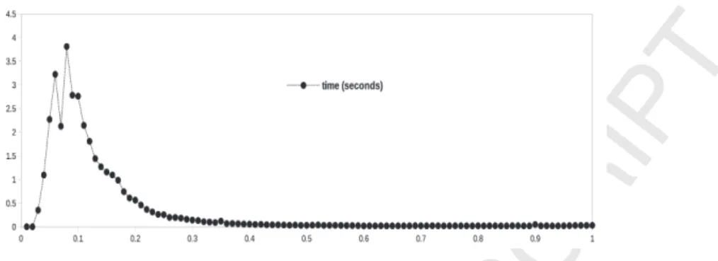
EXP 1. We examined how our algorithms perform as|R|changes. Figure 7 illus-trates the behavior of algorithm 4 running on a set of 1000afs. Theseafs were generated randomly with|A|= 120 in each instance. Every point of the chart of figure 7 represents the average running time of solving 10afs. For everyp∈ {0.01,0.02,0.03, ...,0.98,0.99,1.0}, we generated 10 random afs using p as the probability of any (x, y) being in R for a given af. More specifically, given a set of argumentsA={a0, a1, ..., a118, a119}then the probability thatai∈Aattacksaj∈Ais equal top. Back to figure 7, we observed two facts:
(a) hard (random) afs for algorithm 4 (and analogously for all of the algorithms of this paper) might be often among those instances with (approximately) 2|A| < |R| < 20|A|. Nonetheless, we stress that not every af (with 2|A| < |R| < 20|A|) is necessarily hard to our algorithm.
(b) the running-time of the algorithms is more sensitive to |R| rather than|A|, which is also observed in [8, 10].
EXP 2. We compared the running-time of the new algorithm with the previous algorithm together with two reduction-based solvers: CoQuiAAS and ArgSemSAT, which achieved first (respectively second) place in the First International Competition on Computational Models of Argument (IC-CMA 2015), see [22, 23]. CoQuiAAS is based on constraint program-ming solvers, while ArgSemSAT is based on satisfiability solvers. In this experiment we generated 1000 afs with |A| = 120. For every p ∈
Figure 7: The behavior of algorithm 4 where the x-axis represents the probability used in generating the corresponding solvedafs.
Table 1: The results of EXP 2 that verify the new looking-ahead strategy.
problem new algorithms previous algorithms CoQuiAAS ArgSemSAT seconds timeouts seconds timeouts seconds timeouts seconds timeouts
P1preferred 241.83 0 11813.50 68 66.80 0 1356.17 0 P1stable 90.35 0 1239.33 0 30.27 0 2302.99 0 P1complete 227.32 0 11715.29 69 48.26 0 1449.92 0 P1admissible 2553.70 7 - - - -P1semi stable 247.68 0 11764.22 70 - - - -P1ideal 244.70 0 11798.88 70 - - - -P3preferred 26.06 0 51.97 0 7.21 0 78.47 0 P4preferred 69.81 0 3097.94 21 36.94 0 109.69 0 P3stable 21.54 0 - - 2.06 0 92.51 0 P4stable 50.80 0 - - 6.63 0 118.57 0
as the probability of any (x, y) being inR for a givenaf. We report the total running-time of solving the 1000 afs in table 1. We use (-) in the tables to imply that a problem is not solvable by the respective solver. In summary, the table verifies that the new algorithms are more efficient than previous algorithms. In this experiment we note that the total running-times of ArgSemSAT are larger than the new algorithms. However it does not contradict the results of ICCMA 2015. This is because most of the afs of the competition seem to be generated with 2|A| < |R| < 20|A|, which are hard to our algorithms as we noted earlier.
EXP 3. Comparing with CoQuiAAS and ArgSemSAT, we evaluated the perfor-mance of the new algorithms using a different set of random afs. We generated 1000 random afs with |A|=120 as illustrated next. Given a set of argumentsA={a0, a1, a3, ..., a118, a119}, then the probability that ai ∈ A attacks aj ∈ A is equal to 0.01 + 0.01∗(i div 2). Thereby the number of outgoing attacks varies from argument to argument in a given af. This is in contrary to the generated afs for the other experiments where in a givenafthe number of outgoing attacks is almost constant for all arguments. We report the total running-times of solving the 1000afs in table 2. The results show that the evaluatedafs are easier to the new algorithm than the set used in EXP 2. This confirms that hard random
Table 2: The results of EXP 3, using a different set of randomafs.
problem new algorithms CoQuiAAS ArgSemSAT
seconds timeouts seconds timeouts seconds timeouts
P1preferred 20.10 0 20.98 0 199.81 0 P1stable 17.32 0 16.93 0 172.38 0 P1complete 27.91 0 13.11 0 233.55 0 P1admissible 28.29 0 - - - -P1semi stable 28.12 0 - - - -P1ideal 20.00 0 - - - -P3preferred 10.00 0 0.89 0 30.88 0 P4preferred 10.09 0 6.02 0 40.19 0 P3stable 10.41 0 7.05 0 30.83 0 P4stable 14.96 0 12.50 0 39.62 0
Table 3: The results of EXP 4, using randomafs with|A|=200.
problem new algorithms CoQuiAAS ArgSemSAT
seconds timeouts seconds timeouts seconds timeouts
P1preferred 1917.12 12 765.81 1 1533.24 1 P1stable 1353.48 6 180.89 0 1745.36 2 P1complete 1906.85 12 316.69 0 1733.77 1 P1admissible 2017.41 14 - - - -P1semistable 1904.54 12 - - - -P1ideal 1901.50 12 - - - -P3preferred 85.16 0 11.40 0 53.70 0 P4preferred 1072.22 6 397.88 1 109.06 0 P3stable 132.67 0 5.24 0 53.19 0 P4stable 289.89 1 44.38 0 124.87 0
afs are often among those with 2|A| < |R| < 20|A|. Note that in this experiment the average probability used in generating the afs is about 0.3, which means on average|R|>30|A|.
EXP 4. In contrast to CoQuiAAS and ArgSemSAT, we evaluated how the new algorithms perform as|A|increases. Therefore, we generated 100 random afs with |A|=200. For every p ∈ {0.01,0.02,0.03, ...,0.98,0.99,1.0}, we generated an af using p as the probability of any (x, y) being inR. In table 3 we report the total running-times of solving the 100 afs. As we expected, the total times of our algorithms go up as the number of arguments grows.
6. Conclusion
We have presented refined backtracking algorithms for computational prob-lems under a number of argumentation semantics: preferred, admissible,
com-plete, stable, semi stable and ideal semantics. Specifically, we improved the backtracking search for extensions by using a global looking-ahead strategy rather than the local looking-ahead strategy used in existing backtracking al-gorithms [19]. Also, we set a new implementation of a backtracking approach to deciding the acceptance problem –withoutnecessarily listing all extensions– under preferred, complete, admissible and stable semantics. All presented algo-rithms are implemented and the improvements are experimentally verified.
The paper was focused on improving backtracking-based implementations for abstract argumentation frameworks. This line of research, i.e. backtracking algo-rithms forafs, was considered by a number of works such as [10, 11, 7, 25, 4, 21]. However, we build on the state-of-art backtracking-based implementations pre-sented in [19, 18]. There are, of course, different kinds of implementation such as reduction-based algorithms; see [9] for an excellent review of methods for implementing computational problems in abstract argumentation. Additionally the results of ICCMA 2015 [22] show the performance of some of the above al-gorithms compared with reduction-based methods; our entry in the competition was under the name “ArgTools”. Although the presented backtracking-based implementations might not be as efficient as some reduction-based solvers, we believe it is a matter of time until more intelligent backtracking techniques will be implemented for abstract argumentation. In this regard, we plan to investigate implementing backtracking procedures that learn from failures (i.e. dead-ends). Such learning process is an important factor in the efficient backend solvers of the successful reduction-based entries of ICCMA 2015, see for exam-ple [1, 15]. Also in future work we will study different dynamic orderings for the argument selection. Recall the presented algorithms apply a static ordering, which depends on the number of neighbor arguments.
Acknowledgements
The authors thank the anonymous reviewers for the helpful comments that led to an improved presentation. We also thank Stefan Woltran (from Vienna University of Technology) for the useful discussion via email on issues related to implementing abstract argumentation. The research of the first author, Samer Nofal, is supported by the Scientific Research Deanship at German Jordanian University (project number SIC 18/2015.)
References
[1] Gilles Audemard and Laurent Simon. Predicting learnt clauses quality in modern SAT solvers. InIJCAI 2009, Proceedings of the 21st International Joint Conference on Artificial Intelligence, Pasadena, California, USA, July 11-17, 2009, pages 399–404, 2009.
[2] Pietro Baroni, Martin Caminada, and Massimiliano Giacomin. An intro-duction to argumentation semantics. Knowledge Eng. Review, 26(4):365– 410, 2011.
[3] Trevor J. M. Bench-Capon, Katie Atkinson, and Adam Zachary Wyner. Using argumentation to structure e-participation in policy making. T. Large-Scale Data- and Knowledge-Centered Systems, 18:1–29, 2015. [4] Martin Caminada. An algorithm for computing semi-stable semantics. In
Symbolic and Quantitative Approaches to Reasoning with Uncertainty, 9th European Conference, ECSQARU 2007, Hammamet, Tunisia, October 31 - November 2, 2007, Proceedings, pages 222–234, 2007.
[5] Martin Caminada, Walter Alexandre Carnielli, and Paul E. Dunne. Semi-stable semantics. J. Log. Comput., 22(5):1207–1254, 2012.
[6] Martin W. A. Caminada and Dov M. Gabbay. A logical account of formal argumentation. Studia Logica, 93(2-3):109–145, 2009.
[7] Claudette Cayrol, Sylvie Doutre, and J´erˆome Mengin. On decision prob-lems related to the preferred semantics for argumentation frameworks. J. Log. Comput., 13(3):377–403, 2003.
[8] Federico Cerutti, Paul E. Dunne, Massimiliano Giacomin, and Mauro Val-lati. Computing preferred extensions in abstract argumentation: A sat-based approach. In Theory and Applications of Formal Argumentation -Second International Workshop, TAFA 2013, Beijing, China, August 3-5, 2013, Revised Selected papers, pages 176–193, 2013.
[9] G¨unther Charwat, Wolfgang Dvor´ak, Sarah Alice Gaggl, Johannes Peter Wallner, and Stefan Woltran. Methods for solving reasoning problems in abstract argumentation - A survey. Artif. Intell., 220:28–63, 2015.
[10] Yannis Dimopoulos, Vangelis Magirou, and Christos H. Papadimitriou. On kernels, defaults and even graphs. Ann. Math. Artif. Intell., 20(1-4):1–12, 1997.
[11] Sylvie Doutre and J´erˆome Mengin. Preferred extensions of argumentation frameworks: Query answering and computation. InAutomated Reasoning, First International Joint Conference, IJCAR 2001, Siena, Italy, June 18-23, 2001, Proceedings, pages 272–288, 2001.
[12] Phan Minh Dung. On the acceptability of arguments and its fundamental role in nonmonotonic reasoning, logic programming and n-person games.
Artif. Intell., 77(2):321–358, 1995.
[13] Phan Minh Dung, Paolo Mancarella, and Francesca Toni. Computing ideal sceptical argumentation. Artif. Intell., 171(10-15):642–674, 2007.
[14] Paul E. Dunne. Computational properties of argument systems satisfying graph-theoretic constraints. Artif. Intell., 171(10-15):701–729, 2007.
[15] Niklas E´en and Niklas S¨orensson. An extensible sat-solver. In Theory and Applications of Satisfiability Testing, 6th International Conference, SAT 2003. Santa Margherita Ligure, Italy, May 5-8, 2003 Selected Revised Pa-pers, pages 502–518, 2003.
[16] Luca Longo and Pierpaolo Dondio. Defeasible reasoning and argument-based systems in medical fields: An informal overview. In 2014 IEEE 27th International Symposium on Computer-Based Medical Systems, New York, NY, USA, May 27-29, 2014, pages 376–381, 2014.
[17] S. Modgil, F. Toni, F. Bex, I. Bratko, C.I. Ches˜nevar, W. Dvoˇr´ak, M.A. Falappa, X. Fan, S.A. Gaggl, A.J. Garc´ıa, M.P. Gonz´alez, T.F. Gordon, J. Leite, M. Moˇzina, C. Reed, G.R. Simari, S. Szeider, P. Torroni, and S. Woltran. The added value of argumentation. In Sascha Ossowski, edi-tor,Agreement Technologies, volume 8 ofLaw, Governance and Technology Series, pages 357–403. Springer Netherlands, 2013.
[18] Samer Nofal, Katie Atkinson, and Paul E. Dunne. Algorithms for ar-gumentation semantics: Labeling attacks as a generalization of labeling arguments. J. Artif. Intell. Res. (JAIR), 49:635–668, 2014.
[19] Samer Nofal, Katie Atkinson, and Paul E. Dunne. Algorithms for decision problems in argument systems under preferred semantics. Artif. Intell., 207:23–51, 2014.
[20] Nouredine Tamani, Patricio Mosse, Madalina Croitoru, Patrice Buche, Val´erie Guillard, Carole Guillaume, and Nathalie Gontard. An argumenta-tion system for eco-efficient packaging material selecargumenta-tion. Computers and Electronics in Agriculture, 113(0):174 – 192, 2015.
[21] Phan Minh Thang, Phan Minh Dung, and Nguyen Duy Hung. Towards a common framework for dialectical proof procedures in abstract argumen-tation. J. Log. Comput., 19(6):1071–1109, 2009.
[22] Matthias Thimm and Serena Villata. System descriptions of the first in-ternational competition on computational models of argumentation (ic-cma’15). CoRR, abs/1510.05373, 2015.
[23] Matthias Thimm, Serena Villata, Federico Cerutti, Nir Oren, Hannes Strass, and Mauro Vallati. Summary report of the first international compe-tition on computational models of argumentation. AI Magazine, 37(1):102, 2016.
[24] Bart Verheij. Two approaches to dialectical argumentation: admissible sets and argumentation stages. InProceedings of the Eighth Dutch Conference on Artificial Intelligence, pages 357–368, 1996.
[25] Bart Verheij. A labeling approach to the computation of credulous ac-ceptance in argumentation. In IJCAI 2007, Proceedings of the 20th In-ternational Joint Conference on Artificial Intelligence, Hyderabad, India, January 6-12, 2007, pages 623–628, 2007.
![Figure 5: An example to show the enhancement of algorithm 4 over the state-of-the-art algorithm presented in [19].](https://thumb-us.123doks.com/thumbv2/123dok_us/11081968.2994731/15.918.281.765.219.709/figure-example-enhancement-algorithm-state-art-algorithm-presented.webp)