Accepted
Article
inlabru
: an R package for Bayesian spatial modelling from
ecological survey data
Fabian E. Bachl
1, Finn Lindgren
1, David L. Borchers
2,*, and Janine B. Illian
21
School of Mathematics, James Clerk Maxwell Building, The King’s Buildings, Peter Guthrie
Tait Road City, Edinburgh, EH9 3FD, Scotland
2
Centre for Research into Ecological and Environmental Modelling, School of Mathematics
and Statistics, University of St Andrews, The Observatory, St Andrews, Fife, KY16 9LZ,
Scotland
*
Corresponding author: [email protected]
1
Summary
1. Spatial processes are central to many ecological processes, but fitting models that incorporate spatial correlation to data from ecological surveys is computationally challenging. This is particularly true of point pattern data (in which the primary data are the locations at which target species are found), but also true of gridded data, and of georeferenced samples from continuous spatial fields.
2. We describe here theRpackageinlabruthat builds on the widely-usedR-INLApackage to provide easier access to Bayesian inference from spatial point process, spatial count, gridded, and georeferenced data, using integrated nested Laplace approximation (INLA, Rue et al., 2009).
3. The package povides methods for fitting spatial density surfaces and estimating abundance, as well as for plotting and prediction. It accommodates data that are points, counts, georeferenced samples, or distance sampling data.
4. This paper describes the main features of the package, illustrated by fitting models to the gorilla nest data contained in the packagespatstat(Baddeley & Turner, 2005), a line transect survey data set contained in the packagedsm(Milleret al., 2018), and to a georeferenced sample from a simulated continuous spatial field.
Keywords: Spatial modeling, point process, spatial count, georeferenced data, Bayesian inference
This article has been accepted for publication and undergone full peer review but has not been
through the copyediting, typesetting, pagination and proofreading process, which may lead to
differences between this version and the Version of Record. Please cite this article as doi:
Accepted
Article
2
Introduction
Many ecological datasets exhibit spatial correlation in observed variables, due to biotic or abiotic processes such as dispersal limitation, social aggregation, and spatial structure in unobserved explanatory variables. Whether the observations are points (e.g. animal locations), counts (e.g. the numbers of animals in spatial samples) or values of some continuous variable (e.g. nutrient levels at sampled points), spatial correlation causes every observation to depend on every other observation within some unknown correlation range. Dealing with this requires models that are mathematically more complex and computationally more demanding than is the case when there is independence among observations.
We account for spatial dependence by incorporating a Gaussian random field (GRF) into models. GRFs are spatially continuous random processes in which random variables at any point in space are normally distributed and are correlated with random variables at other points in space according to a continuous correlation process. GRFs provide a means of modelling the spatial signal in the observations that cannot be accounted for by covariates.
In the case of point data and count data, the GRF is linked to the response variable by a log link function, to give a log Gaussian Cox process (LGCP) model (Møller & Waagepetersen, 2007). (Called “log Gaussian” because the log of the intensity at any point is assumed to be normally distributed, and “Cox process” because a Poisson process that has a randomly varying intensity function is called a Cox process.) What spatial statisticians call the “intensity” is the density in our context, and we will use the term “density” for this henceforth.
The GRF is approximated by the solution to a stochastic partial differential equation (SPDE; see Lindgren
et al., 2011, for details). We do not have space to describe the details of SPDEs, but fortunately the mathematical
details need not be understood to use them ininlabru. It is sufficient to know that SPDEs provide an efficient way of approximating the GRF in continuous space (Simpsonet al., 2016).
Integrated nested Laplace approximation (INLA) Bayesian methods (Rueet al., 2009) are used for inference. INLA is a fast and accurate alternative to Markov chain Monte Carlo (MCMC) for fitting latent Gaussian models, i.e., hierarchical models in which there are unobserved (latent) normally distributed random variables. The models we consider here, in which the GRF is latent, are of this type. We refer the reader to the “Gentle INLA tutorial” athttps://www.precision-analytics.ca/blog-1/inlafor more about INLA, and to the R-INLA project athttp://www.r-inla.org/for more about theR-INLApackage on which theinlabrupackage builds.
The R-INLA package currently requires users to have knowledge of likelihood approximation schemes, and does not allow inference when detection probability is unknown, as is common in many wildlife surveys. The
inlabrupackage makes fitting spatial models with INLA more accessible to non-specialist users by employing simpler syntax, and it extends the class of models that can be fitted to include distance sampling.
We illustrate the scope of the package by fitting models to point and count data from a survey of gorilla
Accepted
Article
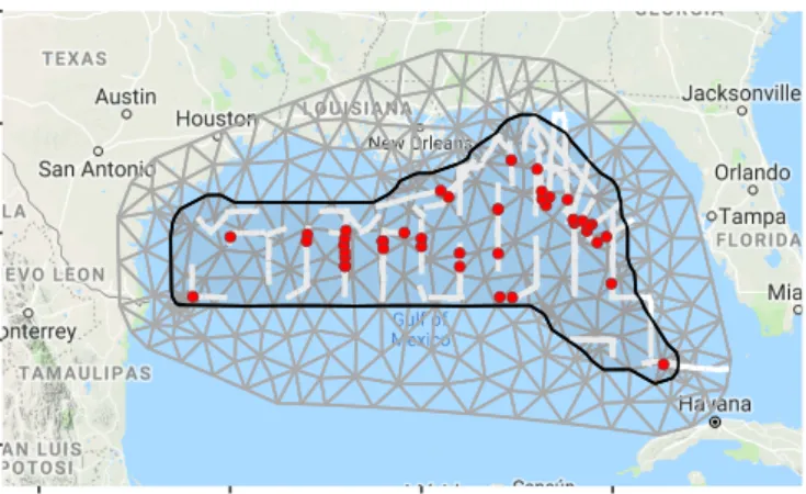
22.5 25.0 27.5 30.0 32.5 −100 −95 −90 −85 lon latFigure 1: Pantropical dolphin survey data plotted using ggmap and thegm method. Grey triangles show the
inla.mesh object. The survey region boundary (black) is held in a SpatialPolygonsDataFrame. The line transects (white lines) are held in aSpatialLinesDataFrameand the detected dolphins (red points) are held in aSpatialPointsDataFrame.
attenuata)1, and a simulated survey of a continuous spatial field. Other examples can be found at
http: //inlabru.org/tutorials.
3
Data format and visualization
The inlabru package supports the sp package data structures (Pebesma & Bivand, 2005). These are well documented withinsp, togeher with powerful functions for manipulating them. TheSpatialPointsDataFrame
structure stores spatial points together with spatial covariate data and attributes of points (e.g. size or species).
SpatialLinesDataFrames store spatial data for line transect surveys and SpatialPolygonsDataFrames are used to define survey regions and sample plots.
Continuous space is approximated in inlabruusing a “mesh” (a tiling of space with triangular tiles – see Figure 1 for example). We use theinla.meshclass of object from theINLApackage for this approximation.
Data visualization tools ininlabruare built on theggplot2(Wickham, 2009) andggmap(Kahle & Wickham, 2013) packages, with customized inlabrufunctions such as ggand gmto extend their functionality. Figure 1 shows an example of such a plot generated from a line transect survey of pantropical spotted dolphins in the Gulf of Mexico.
4
Key syntax
Models are defined by specifying
1. aformulafor the linear or nonlinear predictor that defines the log density function,
2. the components of this predictor (one of which is typically an SPDE), and 3. the observed variable distribution.
Accepted
Article
0 0 0 0 0 0 2 0 0 0 0 10 40 17 7 0 2 41 43 60 0 0 11 5 0 0 0 0 (a) (b) (c) (d)Figure 2: Analysis of gorilla nests as a count and as a point process model. Panel (a) depicts the survey region, search plots, undetected (blue) and detected (red) nests, and the nest counts (white boxes). Panel (b) shows a density fit withbruto nest counts, associating counts with the plot centres. Panels (c) and (d) show point process fits obtained withlgcpusing only nests within the plots, and using all nests, respectively.
Models are fitted using the functionbru( )or, for LGCP models,lgcp( ). Examples are given below.
5
Spatial count data
We begin by usinginlabruto infer a smooth spatial density surface from plot samples in which the response is the count of gorilla nests in each plot (see Figure 2 (a)). Although the exact locations of all nests were recorded, we initially use only nest counts in a sample of plots. The R code showing how to load the package and the data is provided as Supporting Information S1.
The observed response, count, is the number of nests in a plot, which we assume to be a Poisson random variable. We also assume that the log density of the Poisson distribution varies in space and is the sum of an intercept term (the base log density) and an SPDE (which captures the spatially correlated variation about the base). We name the SPDEspat2. Recall that the SPDE approximates a GRF, and we specify below that the correlation of this field has a Mat´ern correlation structure. This correlation model (with unknown parameters) is specified using the INLA functioninla.spde2.matern. The SPDE and correlation model are defined on a
mesh, which we do not show here because it obscures important elements of the plots (see Figure 1 for an example of a mesh).
The two components of our linear predictor are the intercept and the SPDE. We store these in an object calledcmpas follows:
Accepted
Article
cmp <- count ~ spat(map = coordinates, model = inla.spde2.matern(mesh)) + Intercept
The syntax for defining SPDEs requires a name for the SPDE (“spat” here), followed by specification, in brackets, of the domain on which it is defined (“map=coordinates” here), and its correlation function (“model=inla.spde2.matern(mesh)” here). Note that coordinates is a method defined by the package sp
to extract locations from sp spatial objects. Using it as above specifies that the SPDE applies to spatial coordinates.
We use theinlabrufunctionbruto fit the model to the gorilla count datagcounts(aSpatialPointsDataFrame
with a data fieldcountcontaining the nest count data):
fit <- bru(components = cmp,
family = "poisson",
data = gcounts,
formula = ~ spat + Intercept,
options = list(E = gcounts$exposure))
Thecomponentsparameter specifies the model components. Thefamilyparameter specifies the probability density function (PDF) of the response. (Allfamily types supported by the INLA package are supported by
inlabru.) Theformulaspecifies how the components are combined to create a linear (in this case) predictor for density. The parameterEin theoptionslist sets the “exposure” parameter of the Poisson family, namely the areas of each searched plot in this example. (The log of the exposure would be an offset in a Poisson generalised linear model.)
We did not need to specify theformulaabove, becauseinlabruassumes that it is the sum of the components if noformulais given. Theformulais really only required when it is not this sum (see examples in Sections 6.2 and 6.3 below).
We can predict any function of any subset of the components of the model specification (cmpabove) using
inlabru’spredictfunction. For example, predictions of the density are obtained as follows:
pxl <- pixels(mesh, mask = boundary)
dens <- predict(fit, pxl, formula = ~ exp(spat + Intercept))
The first line creates a regular grid of locations covering the survey region. The third argument of the
predict call specifies what is to be predicted, as a function of the components. To predict on the scale of the linear predictor, for example, we would just replace exp(spat+Intercept) with spat+Intercept. The
predictfunction estimates the posterior densities of whatever function is specified in itsformulaargument. The object obtained frompredictis aSpatialPixelsDataFrame. As with any other spatial object, we can employ theggfunction to add it to a blank plot. Hence, callingggplot() + gg(dens)will render the density shown in Figure 2 (b).
Accepted
Article
6
Fitting point processes
We now consider the case in which the data are the locations of nests within plots. Some information about the spatial process governing nest locations is lost when locations are aggregated into counts within plots, and we would like to use all the information in the data. In this case, the response variables are the coordinates of the individual nests, and these locations are random variables, whereas with count data the locations of the plots were fixed and known and the counts were random variables. Spatial point processes models (Møller & Waagepetersen, 2007; Illian et al., 2008; Baddeley et al., 2015) are used when the points themselves are the random variables. More specifically, we use an LGCP, in which the log density includes a GRF, to model overdispersion and clustering that cannot be accounted for by covariates.
6.1
Inference for spatial Poisson point processes
The work flow of inference in point processes fitting is similar to that described above. We specify the model by replacing the user-defined response “count” on the left of the component specification, with the key word “coordinates” to indicate that the responses are spatial coordinates.
cmp <- coordinates ~ spat(map = coordinates, model = inla.spde2.matern(mesh)) + Intercept
The R code showing how to load the data is provided in Supporting Information S1. Fitting an LGCP model is done usinglgcp:
fit <- lgcp(components = cmp, data = plotnests, samplers = plots)
Hereplotnestsis aSpatialPointsDataFramecontaining the locations of the observed nests. Thesamplers
argument is passed aSpatialPolygonsDataFramecalledplotsthat specifies the polygons that were searched. If this argument is left empty,lgcp will assume that the whole domain defined by the mesh (contained in the SPDE specification,spat, incmp) was searched, which would result in biased inference if the whole domain was not searched.
Running the code above and then usingpredictandplotyields the density plot shown in Figure 2 (c). For comparison, Figure 2 (d) shows a LGCP fit to the complete gorilla nest data set, which was obtained as above but withsamplers=boundary in place of samplers=plots, whereboundaryis a SpatialPolygonsDataFrame
object defining the survey boundary.
6.2
Inference for univariate point processes: distance sampling detection function
We illustrateinlabru’s ability to model one-dimensional point processes by fitting a detection function to the perpendicular distances of detected dolphins on the line transect survey shown in Figure 1. TheRcode showing how to load and prepare the data is provided as Supporting Information S2.
The observed density of distances to detections is the product of the underlying density of distances to dol-phins (λ(d) say, wheredis distance) and the probability of detecting a dolphin that is at distanced(h(d; log{σ})
Accepted
Article
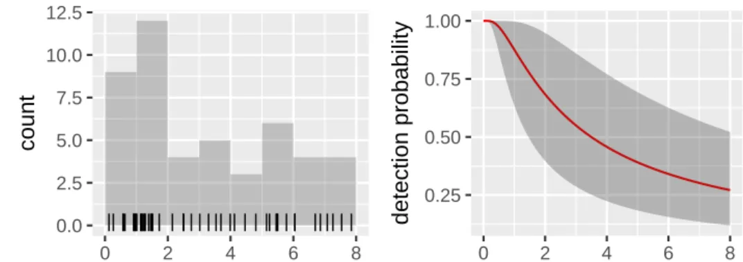
| ||| || | || | | | | ||| || |||||||| ||| ||| | |||||||| || ||| | 0.0 2.5 5.0 7.5 10.0 12.5 0 2 4 6 8distance
count
0.25 0.50 0.75 1.00 0 2 4 6 8distance
detection probability
Figure 3: Pantropical dolphin detection distances (left) and fitted hazard rate detection function (right), showing 95% credibile region. With adequate fit, the red line is a smooth through the histogram, as is apparent here.
say, where log{σ} is an unknown parameter). Under the usual line transect assumption that animals are uni-formly distributed with respect to distance from the line,λ(d) =λso that the density of the observed distance process ish(d; log{σ})λ. Hence the log density can be written as log[h(d; log{σ})] +β0, whereλ=eβ0.
We specify the (nonlinear) predictor for this model, and its components, as follows:
fml <- distance ~ log(h(distance, lsig)) + Intercept cmp <- distance ~ lsig + Intercept
where h(distance,lsig)is h(d,log{σ}) and Interceptis β0= log(λ). To complete the specification we
need to define the functionh(distance,lsig). We define it to be the hazard-rate detection function of Hayes & Buckland (1983), with shape parameter 1, as follows:
h <- function(distance, lsig){ 1-exp(-(distance/(exp(lsig)))^-1)}.
Because one of the components (the parameter lsig) enters the linear predictor for log density via a non-linear function, log[h(d; log{σ})], we need to specify theformulaexplicitly, rather than haveinlabruconstruct it by default as the sum of thecomponents. This model is fitted usinglgcp as follows:
fit <- lgcp(cmp, mexdolphin$points, formula = fml).
where mexdolphin$pointsis a SpatialPointsDataFramewith a variabledistancefor every point. After fitting the model, predicting the detection function for distances 0 to 8 (the maximum distance considered) is straightforward using
pts <- data.frame(distance = seq(0,8, by = 0.1)), dfun <- predict(fit, pts, formula = ~ h(distance, lsig)
whileplot(dfun) plots it with 95% credible interval (as shown in Figure 3).
We note in passing thatinlabrucan be used to estimateany PDF using commands similar to those above, if we consider the intensity of a Poisson process to be an unnormalized PDF.
Accepted
Article
6.3
Inference for thinned Poisson processes: distance sampling
We now useinlabruto estimate the density and distribution of dolphin groups with the conventional distance sampling assumption of uniform group distribution within searched strips. This assumption is tenable because the searched strips have negligible width compared to the size of the survey region (see Figure 1) and were laid down with random start location. We implement the assumption by simultaneously modelling the spatial distribution of detected points (as in Section 6.1) and the PDF of distances of detections from the lines, assuming uniform distribution of these distances (as in Section 6.2). The R code for this is provided as Supporting Information S4.
An analysis of these data (also assuming uniform group distribution within searched strips) using the R pack-agedsmis available athttp://distancesampling.org/R/vignettes/mexico-analysis.html. The methods implemented ininlabruanddsmdiffer in a number of ways, including thatinlabruimplements a fully-Bayesian approach, so one can specify priors on parameters (not illustrated here), andinlabruestimates detection prob-ability and the density surface simultaneously, while dsmestimates detection probability in one step and the density surface conditional on this estimate, in another.
The key to simultaneous estimation of detection probability and the density surface is the fact that if the locations of points arise from a Poisson process, then the locations of the detected points arise from a
thinned Poisson process. “Thinning” involves detecting points with some probability (h, say) that is less than
1. The density (intensity) of a thinned Poisson process is the unthinned densityD, multiplied by the thinning probability h. For example, if h = 0.5 so that half the points are detected on average, then the density of detected points is half that of the all points: Dh=D/2. On a line transect survey, the probability of missing ˚a point depends on its distancedfrom the line, so thathis a function of distance (h(d)) and the density of the thinned Poisson process at the point’s location is Dh(d), where D is the underlying density at this location. WritingDasD= exp(Intercept) and noting thatDh(d) = exp(Intercept+ log(h(d)), we see that the log density of the thinned Poisson process is equal to the log density of the underlying process plus the log of the detection probability. This is convenient, because it means that we can do inference for thinned LGCPs by simply adding a term for the thinning probability to the log density.
With this in mind, and noting that the thinning probability has an unknown parameter that we calllsig, we specify our model by combining thecomponents specification andformulaspecifications from Sections 6.1 and 6.2.
cmp <- ~ spat(map = coordinates, model = inla.spde2.matern(mesh)) + lsig + Intercept fml <- coordinates + distance ~ spat + log(h(distance, lsig)) + log(1/8) + Intercept
The left hand side of the formula (coordinates + distance) tellsinlabruthat we are modelling both the spatial point process governing dolphin group locations, and the detection distances. The right hand side says that the log density of this process is the sum of the log detectability and the spatial process composed of the spatial SPDE, and the Intercept. The offset term log(1/8) specifies that the density of distances is assumed
Accepted
Article
−1750
−1500
−1250
−1000
0
500
1000
Easting
Nor
thing
0.00050 0.00075 0.00100 0.00125mean
Figure 4: Predicted density surface (in counts per square km) of a point process model for dolphin groups fitted jointly with a hazard rate detection function (not shown).
to be constant on the distance interval (0,8) – as the transect half-width is 8 km.
With the above definitions, fitting the model is straightforward using the same syntax as shown in Section 6.1, where now the samplers argument is a SpatialLinesDataFrame storing the survey’s ship transects. The prediction code introduced in Section 5 is then used to estimate the spatial density surface shown in Figure 4(a). We can add further processes, such as a group size probability model. This allows us to make detection probability depend on group size and to model a spatially varying group size distribution. We do not illustrate this here for lack of space.
7
Georeferenced data from a continuous spatial field
We illustrate spatial modelling from a continuous spatial field by sampling the simulated field (which might cor-respond to a soil nutrient level, for example) shown in Figure 5(a), at the locations of the crosses in that figure. Having specified a Mat´ern correlation function usinginla.spde2.matern in a similar way to that shown pre-viously, and given that the sampled observations are in theobserveddata field of aSpatialPointsDataFrame
namedgeosamp, the model is fitted as follows, assuming a Gaussian error model:
cmp <- observed ~ field(map = coordinates, model = inla.spde2.pcmatern(mesh)) + Intercept fit <- bru(components = cmp, data = geosamp, family = "gaussian")
(Here we have named the SPDE “field” rather than “spat”.)
+ + + + + + + + + + + + + + + + + + + + + + + + + + + + + + + + + + + + + + + + + + + + + + + + + + + + + + + + + + + + + + + + + + + + + + + + + + + + + + + + + + + + + + + + + + + + + + + + + + + + + + + + + + + + + + + + + + + + + + + + + + + + + + + + + + + + + + + + + + + + + + + + + + + + + + + + + + + + + + + + + + + + + + + + + + + + + + + + + + + + + + + + + + + + + + + + + + + + + + + + 0.0 2.5 5.0 7.5 10.0 0.0 2.5 5.0 7.5 10.0 x y
(a) True field
0.0 2.5 5.0 7.5 10.0 0.0 2.5 5.0 7.5 10.0 x y (b) Posterior mean 0.0 2.5 5.0 7.5 10.0 0.0 2.5 5.0 7.5 10.0 x y (c) Posterior sample
Figure 5: (a) A simulated continuous spatial field, showing sample locations, (b) the posterior mean of the model fitted to the sample data, and (c) a sample from the posterior distribution of the field.
Accepted
Article
The mean of the fitted model is shown in Figure 5(b), while a sample from the posterior distribution of the field is shown in Figure 5(c). Note that the mean surface is necessarily smoother than the true field (which is conceptually a draw from a random field with the given mean), while the posterior sample better reflects the fine-scale structure of the true field.
8
Discussion
The inlabrupackage makes Bayesian spatial modelling with INLA, including point process modelling, more accessible to ecologists. It allows one to model species distribution and estimate density and abundance with data that are (a) complete spatial maps of the locations of individuals or groups, (b) counts in plots, (c) points, and (d) distance sampling data.
It is distinguished from methods and software that fit density surfaces to count data in that it can deal with points as responses in continuous space and does not require that space be discretised (althoughinlabrucan deal with such data, as illustrated in Section 5 above). Nor does it require a neighbourhood structure to be defined, as is required for conditional autoregressive models or simultaneous autoregressive models, for example. It also provides a means of doing Bayesian spatial modelling with distance sampling data. Its distance sampling capabilities are not as well developed as those of the frequentist package dsm(Miller et al., 2018), and unlikedsm, it estimates the detection probability and density surface simultaneously. It shares this feature with the frequentist packageunmarked(Fiske & Chandler, 2011), althoughunmarkedhas no spatial modelling capabilities. Simultaneous estimation of detection probability and the density surface is conceptually satisfying, but the jury is out on whether this, or estimation of the two in separate steps, is preferable in practice
Features of inlabru that we do not have space to describe include its ability to do temporal and spatio-temporal modelling and its ability to simultaneously estimate the density of a point process and the spatially-varying density of what spatial statisticians call “marks” on points (dolphin group size, being an example) as well as its impact on the shape of the detection function.
Features under development include point transect data, modelling multi-species density when there is spatial interaction or common explanatory environmental data for the distribution of different species sharing a habitat, and modelling of habitat preference based on telemetry data. There are some technical obstacles to implementing spatial capture-recapture methods (Efford, 2004; Borchers & Efford, 2008; Royle & Young, 2008) ininlabru, but work in this area is ongoing.
Acknowledgments
Accepted
Article
Data Accessibility
All data used in this paper are available in theR packageinlabru, which can be downloaded from the Com-prehensive R Archive Network athttps://cran.r-project.org/web/packages/inlabru/index.html.
Supplementary Material
RMarkdown scripts:
• Supporting Information S1: 1 spatial gorilla models.Rmd. Code for spatial Poisson count and LGCP inference.
• Supporting Information S2: 2 dfun univariate.Rmd. Code for detection function inference.
• Supporting Information S3: 3 distsamp.Rmd. Code for line transect models.
• Supporting Information S4: 4 georefsim.RmdCode for models for georeferenced data.
Author contributions statement
FB, DB, JI and FL conceived the ideas and designed methodology; FB and DB analysed the data; FB and FL wrote the code, with a minor contribution from DB; FB led the writing of the manuscript, with major contributions from all authors.
References
Baddeley, A., Rubak, E. & Turner, R. (2015)Spatial point patterns: methodology and applications with R. CRC Press.
Baddeley, A. & Turner, R. (2005) spatstat: An R package for analyzing spatial point patterns. Journal of
Statistical Software,12, 1–42.
Borchers, D.L. & Efford, M.G. (2008) Spatially explicit maximum likelihood methods for capture-recapture studies. Biometrics, 64, 377–385.
Efford, M.G. (2004) Density estimation in live-trapping studies. Oikos,106, 598–610.
Fiske, I. & Chandler, R. (2011) unmarked: An R package for fitting hierarchical models of wildlife occurrence and abundance. Journal of Statistical Software,43, 1–23.
Funwi-Gabga, N. (2008) A pastoralist survey and fire impact assessment in the Kagwene Gorilla Sanctuary. Master’s thesis, Geology and Environmental Science, University of Buea, Cameroon.
Hayes, R.J. & Buckland, S.T. (1983) Radial-distance models for the line-transect method. Biometrics, 39(1), 29–42.
Accepted
Article
Illian, J.B., Penttinen, A., Stoyan, H. & Stoyan, D. (2008)Statistical Analysis and Modelling of Spatial Point
Patterns. Wiley, Chichester.
Kahle, D. & Wickham, H. (2013) ggmap: Spatial visualization with ggplot2. The R Journal,5, 144–161. Lindgren, F., Rue, H. & Lindstr¨om, J. (2011) An explicit link between Gaussian fields and Gaussian Markov
random fields: the SPDE approach (with discussion). Journal of the Royal Statistical Society: Series B,
73(4), 423–498.
Miller, D.L., Rexstad, E., Burt, L., Bravington, M.V. & Hedley., S. (2018)dsm: Density Surface Modelling of
Distance Sampling Data. R package version 2.2.16.
Møller, J. & Waagepetersen, R.P. (2007) Modern statistics for spatial point processes (with discussion).
Scan-dinavian Journal of Statistics,34, 643–711.
Pebesma, E.J. & Bivand, R.S. (2005) Classes and methods for spatial data in R. R News,5, 9–13.
Royle, J.A. & Young, K.V. (2008) A hierarchical model for spatial capture-recapture data. Ecology,89, 2281– 2289.
Rue, H., Martino, S. & Chopin, N. (2009) Approximate Bayesian inference for latent Gaussian models by using integrated nested Laplace approximations (with discussion). Journal of the Royal Statistical Society: Series
B,71(2), 319–392.
Simpson, D., Illian, J.B., Lindgren, F., Sørbye, S.H. & Rue, H. (2016) Going off grid: Computationally efficient inference for log-Gaussian Cox processes. Biometrika,103, 49–70.