HILBERT-HUANG TRANSFORM
A thesis presented to the faculty of the Graduate School of
Western Carolina University in partial fulfillment of the
requirements for the degree of Master of Science in Technology.
By
Jieying Han
Director: James Z. Zhang, Ph.D.
Dean & Professor
Department of Engineering and Technology
Committee Members:
Dr. Robert Adams, Department of Engineering and Technology
Professor Paul Yanik, Department of Engineering and Technology
April 2013
c
Firstly, I am sincerely grateful to all the faculty members of Kimmel School for their as-sistance and support during the past two years. My gratitude is extended to my committee members Dr. Robert Adams and Professor Paul Yanik for their guidance and encourage-ment.
I would like to thank Dr. Weiguo Yang, Dr. Julia Barnes, Dr. Michael Smith, Dr. Martin Tanaka and Dr. Steve Ha for their help and advice to my Ph.D. application.
Many thanks go to Jerry Denton, Shawn Lyvers, Nathan Thomas and Michael Jor-dan for their patience and help during my summer internship. Thanks to Alison Krauss and Pat Smith for their assistance. Also thanks go to my classmates who helped with my study. My utmost thanks go to my advisor, Dr. James Z. Zhang. Thank you for every-thing, especially for opening the door of opportunity. Thank you for your encouragement, willingness to help and advice on issues far beyond this degree. You will always be the “King of Advisors” to me.
List of Tables . . . iv List of Figures . . . v Abstract . . . vi CHAPTER 1. Introduction . . . 9 CHAPTER 2. Background . . . 12 2.1 Hilbert-Huang Transform . . . 12
2.1.1 Empirical Mode Decomposition Method . . . 12
2.1.2 Hilbert Spectrum . . . 14
2.1.3 Marginal Spectrum . . . 15
2.1.4 Energy Density Level . . . 15
2.1.5 An Example of HHT . . . 16
2.2 Hurst’s Rescaled-Range(R/S) Method . . . 18
2.3 KDD Cup 1999 Testing Data . . . 19
CHAPTER 3. Novel Detection Methods . . . 25
3.1 Weighted Self-similarity Based on the First IMF . . . 25
3.1.1 Detection Algorithm . . . 25
3.1.2 Attack-Free Reference . . . 27
3.1.3 Detection Criteria . . . 28
3.2 Pearson’s Distance Based on Marginal Spectrum . . . 28
3.2.1 Detection Algorithm . . . 29
3.2.2 Attack-Free Reference . . . 29
3.2.3 Detection Criteria . . . 30
3.3 Rate Change of Energy Density Level . . . 30
3.3.1 Detection Algorithm . . . 30
3.3.2 Detection Criteria . . . 31
CHAPTER 4. Results and Analysis . . . 32
4.1 Pre-treat the Testing Data . . . 32
4.2 Testing Results . . . 32
4.2.1 Weighted Self-similarity Based on the First IMF . . . 32
4.2.2 Pearson’s Distance Based on Marginal Spectrum . . . 39
4.2.3 Rate Change of Energy Density Level . . . 43
CHAPTER 5. Conclusion and Future Work . . . 47
Bibliography . . . 48
APPENDIX A. Testing Results Using Method 1 . . . 54
APPENDIX B. Testing Results Using Method 2 . . . 60
2.1 Basic features of individual TCP connections . . . 21 2.2 Content features within a connection suggested by domain knowledge . . 22 2.3 Traffic features computed using a two-second time window . . . 22 2.4 Basic characteristics of the KDD 99 intrusion detection datasets in terms
of the number of samples . . . 23 2.5 Class labels that appears in the “10% KDD” dataset . . . 24
2.1 EMD Procedures . . . 13
2.2 HHT Procedures . . . 15
2.3 Example of HHT Process . . . 17
3.1 Marginal Spectrum & Pearson’s Distance . . . 29
3.2 Autocorrelation of Energy Density Level . . . 30
3.3 Autocorrelation of Energy Density Level (First Half) . . . 31
4.1 Weighted Self-similarity Example 1: Normal Data . . . 33
4.2 Weighted Self-similarity Example 1: Data With Attacks . . . 34
4.3 Weighted Self-similarity Example 1: All Attacks Data . . . 35
4.4 Weighted Self-similarity Example 1: Attacks Stopped Data . . . 36
4.5 Weighted Self-similarity Example 2: Normal Data . . . 37
4.6 Weighted Self-similarity Example 2: Data With Attacks . . . 37
4.7 Weighted Self-similarity Example 2: All Attacks Data . . . 38
4.8 Weighted Self-similarity Example 2: Attacks Stopped Data . . . 38
4.9 Marginal Spectrum Example 1: Normal Data . . . 39
4.10 Marginal Spectrum Example 1: Data With Attacks . . . 40
4.11 Marginal Spectrum Example 2: Normal Data . . . 41
4.12 Marginal Spectrum Example 2: Data With Attacks . . . 41
4.13 Marginal Spectrum Example 2: All Attacks Data . . . 42
4.14 Marginal Spectrum Example 2: Attacks Stopped Data . . . 42
4.15 Autocorrelation of Energy Density Level Example 1: Normal Data . . . . 43
4.16 Autocorrelation of Energy Density Level Example 1: Data With Attacks . 44 4.17 Autocorrelation of Energy Density Level Example 2: Normal Data . . . . 45
4.18 Autocorrelation of Energy Density Level Example 2: Data With Attacks . 45 4.19 Autocorrelation of Energy Density Level Example 2: All Attacks Data . . 46 4.20 Autocorrelation of Energy Density Level Example 2: Attacks Stopped Data 46
NETWORK TRAFFIC ANOMALY DETECTION USING EMD AND HILBERT-HUANG TRANSFORM
Jieying Han, M.S.T.
Western Carolina University (April 2013) Director: James Z. Zhang, Ph.D.
Empirical Mode Decomposition (EMD) and Hilbert-Huang Transform (HHT) pro-vide a means for adaptive data analysis. EMD extracts Intrinsic Mode Functions (IMFs) that represent the frequency and amplitude characteristics of a signal. HHT generates the marginal spectrum and energy density level of a signal. The IMFs, the marginal spectrum, and the energy density level characterize a signal from three different perspectives.
This thesis proposes three novel parameters for network traffic anomaly detection based on the above three signal characteristics. Hurst parameter of network traffic is cal-culated based on the first IMF, and is expanded by introducing a weighted self-similarity based on the concept of entropy. Pearson’s distance is calculated based on the marginal spectrum to differentiate normal traffic from abnormal ones. Finally, the slopes of cross-correlations are calculated based on the energy density level to detect the rate of energy change between normal and abnormal internet traffic.
CHAPTER 1: INTRODUCTION
Enormous growth of computer network usage and the huge increase in information sharing over the internet have made network security a more and more important field for research. Effective, accurate, and timely detection of network traffic anomaly has become a requirement in the field of information security.
Various schemes are proposed for the network traffic anomaly detection, such as the mode matching approach [1,2], statistical analysis approach [3-8] and Hurst parameter analysis approach [9-11], etc. These approaches have greatly promoted the development of anomaly detection and have improved detection results dramatically. However, due to the complexity of network traffic, no detection model exists that demonstrates both low false positive and low false negative results.
Many researchers have had the idea of using signal processing techniques to detect anomalies in network traffic [12]. Such techniques can detect novel incidents and attacks that cannot be detected by using signature-based approaches. A signature-based approach like SnortR must be updated with new rules in order to recognize new anomalies in net-work traffic. This means such approaches cannot detect new attacks or zero-day attacks that would not be included in the current rules. Signal processing techniques, on the other hand, could be used to detect such attacks. Examples of signal processing techniques include wavelet analysis, entropy analysis, principal component analysis, and spectral analysis.
J.D. Brutlag introduced time series analysis for detecting aberrant behavior through network monitoring by using the Holt-Winters forecasting algorithm [13]. C. M. Cheng proposed a spectral analysis technique to distinguish between normal TCP network traffic and traffic that was dropped or rate-limited by DoS attacks [14]. M. Thottan used signal processing and an abrupt change detection technique in order to detect several anomalies in IP networks [3]. Moreover, Y. Chen applied spectral analysis to TCP flows so as to defend
against reduction of quality attacks [15].
Network traffic entropy analysis has been employed by Y. Gu to detect network traffic anomalies including different kinds of SYN attacks and port scans [16]. A. Wagner used an entropy based method to also detect anomalies and worms propagating in fast IP networks like the Internet backbone [17]. Furthermore, A. Lakhina and B. I. P. Rubin-stein used principal component analysis for diagnosing anomalies in network-wide traffic [18,19]. H. Ringberg discussed the sensitivity of the parameters used in principal compo-nent analysis for network traffic anomaly detection [20].
Wavelet analysis is a well-studied signal processing technique for detecting anoma-lies in network traffic. There are many studies that apply wavelet transformations to net-work traffic. For example, V. Alarcon-Aquino presented an algorithm based on undeci-mated discrete wavelet transform and Bayesian analysis [21]. This algorithm is able to detect and locate subtle changes in variance and frequency in the given time series. Anu Ramanathan presented a WADeS (Wavelet based Attack Detection Signatures) mechanism based on wavelet analysis to detect the DDoS attack [22], which makes wavelet transform for the traffic signals, then computes the variance of the wavelet coefficients to estimate the attack points. Barford presented a method which decomposes network traffic with dec-imated discrete wavelet transform, then synthesizes to Low, Mid, High frequency-parts, and finally detects anomaly with Deviation Scoring [23]. This algorithm is able to detect the flash crowds and short-term anomalies in postmortem. Seong Soo Kim proposed a technique for traffic anomaly detection based on analyzing correlation of destination IP addresses in outgoing traffic at an egress router [24]. This technique can be employed for postmortem and real-time analysis of outgoing network. Lan Li proposed an energy distri-bution based on wavelet analysis to detect the distributed denial-of-service (DDoS) attack [25]. This research showed that the energy distribution variance changes markedly causing a “spike” when traffic behaviors affected by DDoS Attack.
network traffic signalx(t)is stationary. However, the stationarity of network traffic is just an assumption and has no strict mathematical proof. Therefore, the methods mentioned above lack reliable theoretical support [26].
EMD is a new data analysis method developed in recent years. Since the decom-position is based on the local characteristics of the data, it is applicable to non-linear and non-stationary processes. EMD and HHT provide a means for adaptive data analysis. EMD extracts Intrinsic Mode Functions (IMF) that represents the frequency and amplitude char-acteristics of a signal. HHT generates the marginal spectrum and energy density level of a signal. The IMFs, the marginal spectrum, and the energy density level characterize a signal from three different perspectives.
This thesis proposes three novel parameters for internet traffic anomaly detection based on the above three signal characteristics. Hurst parameter of network traffic is cal-culated based on the first IMF, and is expanded by introducing a weighted self-similarity based on the concept of entropy. Pearson’s distance is calculated based on the marginal spectrum to differentiate normal traffic from abnormal ones. Finally, the slopes of cross-correlations are calculated based on the energy density level to detect the rate of energy change between normal and abnormal internet traffic.
The rest of the thesis is organized as follows: Chapter 2 is background theory of HHT method, Hurst’s Rescaled-Range(R/S) model and introduction of our testing data. Chapter 3 introduces and explains the three novel detection methods. Chapter 4 illustrates the testing results through the project. The final chapter provides conclusions and future work.
CHAPTER 2: BACKGROUND
2.1
Hilbert-Huang Transform
Hilbert-Huang Transform is a new method for analyzing nonlinear and non-stationary data. The key part of the HHT is the Empirical Mode Decomposition method with which any complicated data set can be decomposed into a finite and often small number of Intrinsic Mode Functions that admit well-behaved Hilbert transforms [27].
2.1.1 Empirical Mode Decomposition Method
The principle of EMD is to decompose a signal into a sum of IMFs. Each IMF should satisfy the following conditions:
1) In the whole data set, the number of extrema and the number of zero-crossings must either equal or differ at most by one.
2) At any point, the mean value of the envelope defined by the local maxima and the envelope defined by the local minima is zero.
The first condition is similar to the traditional narrow band requirements for a sta-tionary Gaussian process. The second condition is new - its locality is necessary so that the instantaneous frequencies will not have unwanted fluctuations induced by asymmetric waveforms [28].
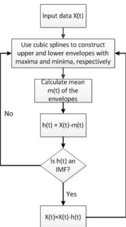
The decomposition process of a signal is an iterative procedure and is described in figure 2.1:
Figure 2.1: EMD Procedures
The EMD procedures can be summarized as follows: Given a signalX(t),(t=1, ...,T)
1) Identify all the maxima and minima ofX(t).
2) Generate its upper and lower envelopes,Xup(t)andXlow(t), with spline interpolation.
3) Calculate the point-by-point mean from upper and lower envelopes,m(t) = [Xup(t) + Xlow(t)]/2.
4) Subtract the mean of the envelopes from the signalX(t)to obtain a new signal,h(t) = X(t)−m(t).
5) Check the properties ofh(t): Ifh(t)meets the above-defined two conditions, an IMF is derived and replaceX(t)with the residualr(t) =X(t)−h(t); Ifh(t)is not an IMF, replaceX(t)withh(t).
6) Repeat Steps 1) - 5) until the residual satisfies given stopping criteria.
At the end of this process, the signalX(t)can be expressed as follows:
X(t) = n
∑
i=1
ci+rn (2.1)
Components c1,c2...cn contain the ingredients from high-frequency to low-frequency of the signal. rncontains trend information of the original signal.
The stopping criterion can be the Standard Deviation (SD) between two consecu-tive results in the sifting process. SD can be expressed as the following equation and the simulation results revealed that the reasonable values are between 0.25∼0.3.
SD= T
∑
t=0 h|hi(k−1)(t)−hik(t)|2 h2i(k−1)(t) i (2.2)In this approach, we only decompose the signal into one IMF and a residue(n=1)since the first IMF provides sufficient information to detect the attacks.
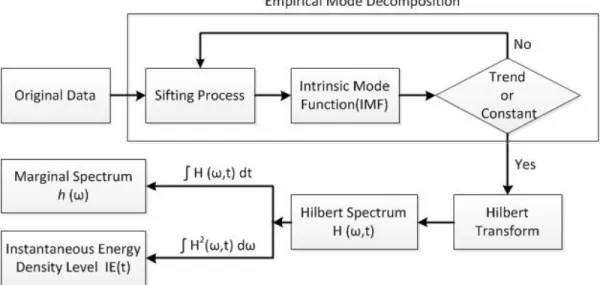
2.1.2 Hilbert Spectrum
After applying the EMD, each IMF is an AM-FM component, which can be processed with the Hilbert Transform:
ˆ ci(t) = 1 π Z +∞ −∞ ci(τ) t−τdτ (2.3)
Whereci(t)is theith IMF, and ˆci(t)is the Hilbert transform ofci(t). With this definition, ci(t)and ˆci(t) form a complex conjugate pair, so we can form the analytic signal of each IMF,zi(t), as: zi(t) =ci(t) +icˆi(t) =ai(t)ejθi(t) (2.4) where ai(t) = [c2i(t) +cˆi2(t)]1/2 θi(t) =arctan ˆ ci(t) ci(t) (2.5)
The instantaneous frequency is given by ωi(t) =dθi(t)/dt , the Hilbert Spectrum of each IMF is defined as:
Hi(ω,t) =ai(t)ejθi(t)=a
i(t)ej R
ωi(t)dt (2.6)
2.1.3 Marginal Spectrum
Hilbert marginal spectrum of theith IMF is defined as:
hi(ω) = Z T
0
Hi(ω,t)dt (2.7)
where T is the duration of the signal,hi(ω)offers a measure of total amplitude (or energy) contribution as a function of frequency, which represents the cumulated amplitude over the entire data span in a probabilistic sense.
2.1.4 Energy Density Level
In addition to the marginal spectrum, the instantaneous energy density level of theith IMF, IEi, is defined as:
IEi(t) = Z
ω
Hi2(ω,t)dω (2.8)
IE depends on time, which can be used to check the energy fluctuation. When attacks occur, the energy will change significantly. That’s why we choose IE as a parameter for detection.
Figure 2.2: HHT Procedures
2.1.5 An Example of HHT
To provide an example of this method, we use the following signal as the input to the algorithm and examine the outputs of the algorithm:
x(t) =cos(2π80t) +0.8 sin(2π50t) +0.6 sin(2π25t) +0.4 cos(2π10t) +0.3 cos(2π3t) (2.9) The signal x(t) contains components with various amplitudes (1, 0.8, 0.6, 0.4, 0.3) and frequencies (80, 50, 25, 10, 3). The goal of this example is to test if the amplitude and frequency contents of the signal can be accurately extracted by the HHT method. As ex-pected, the information was obtained with extreme accuracy. Figure 2.3 (a) is the original signal; figure 2.3 (b) shows the 5 extracted IMFs, each represents one of the expected five components; figure 2.3 (c) shows the Hilbert spectra of IMFs, which clearly shows the five frequencies along the vertical axis and the five amplitudes as individual colors; figure 2.3 (d) shows the marginal spectra and figure 2.3 (e) shows the energy density level of the signal, which is fairly constant because the signal is a sum of periodic signals.
(a) Original Signal
(b) IMFs (c) Hilbert Spectrum
(d) Marginal Spectrum (e) Energy Density Levels
2.2
Hurst’s Rescaled-Range(R/S) Method
Hurst parameter is a conventionally used measure of long-range dependence. There are many methods to estimate the self-similarity parameter H or the intensity of long-range dependence in a time series. In this paper, we use the Rescaled-Range(R/S) method [29].
For a time series, X ={Xi, i≥1}, with partial sumY(n) =∑ni=1Xi, and sample variance S2(n) = (1/n)∑ni=1Xi2−(1/n)2Y2(n), theR/S statistic, or therescaled adjusted range, is given by:
R S(n) = 1 S(n) h max 0≤t≤n Y(t)−t nY(n) − min 0≤t≤n Y(t)−t nY(n) i . (2.10)
For fractional Gaussian noise or fractional ARIMA, the expected value of the R/S statistic is:
E[R
S(n)]vCHn
H (2.11)
asn→∞, whereCH is a positive, finite constant not dependent on n. To determineHusing the R/S statistic, proceed as follows:
1) For a time series of lengthN, subdivide the series intoK blocks, each of sizeN/K.
2) For each lagn, computeR(ki,n)/S(ki,n), starting at pointski=iN/K+1,i=1,2, ..., such thatki+n≤N. For values of n smaller thanN/K, one getsKdifferent estimates ofR(n)/S(n). For values ofnapproachingN, one gets fewer values, as few as 1 when n≥N−N/K.
3) Choosing logarithmically spaced values of n, plot log[R(ki,n)/S(ki,n)] versus logn and get, for each n, several points on the plot. This plot is sometimes called the pox plot for theR/Sstatistic.
4) The parameterH can be estimated by fitting a line to the points in the pox plot.
Since any short-range dependence in the series typically results in a transient zone at the low end of the plot, set a cut-off point, and do not use the low end of the plot for the
purpose of estimating H. Usually, the very high end of the plot is not used as well, because there are too few points on the plot at the high end to make reliable estimates. The values ofnthat lie between the lower and higher cut-off points are used to estimateH.
2.3
KDD Cup 1999 Testing Data
Since 1999, KDD’99 has been the most wildly used dataset for the evaluation of anomaly detection methods [30]. This dataset is prepared by Stolfo et al. [31] and is built based on the data captured in DARPA’98 IDS evaluation program [32]. DARPA’98 is about 4 gigabytes of compressed raw (binary) tcpdump data of 7 weeks of network traffic, which can be processed into about 5 million connection records, each with about 100 bytes. The two weeks of test data have around 2 million connection records. KDD training dataset consists of approximately 4,900,000 single connection vectors each of which contains 41 features and is labeled as either normal or an attack, with exactly one specific attack type. The simulated attacks fall in one of the following four categories:
1) Denial of Service Attack (DoS): is an attack in which the attacker makes some computing or memory resource too busy or too full to handle legitimate requests, or denies legitimate users access to a machine.
2) User to Root Attack (U2R):is a class of exploit in which the attacker starts out with access to a normal user account on the system (perhaps gained by sniffing passwords, a dictionary attack, or social engineering) and is able to exploit some vulnerability to gain root access to the system.
3) Remote to Local Attack (R2L): occurs when an attacker who has the ability to send packets to a machine over a network but who does not have an account on that machine exploits some vulnerability to gain local access as a user of that machine.
4) Probing Attack: is an attempt to gather information about a network of computers for the apparent purpose of circumventing its security controls.
It is important to note that the test data is not from the same probability distribution as the training data, and it includes specific attack types not in the training data which make the task more realistic. Some intrusion experts believe that most novel attacks are variants of known attacks and the signature of known attacks can be sufficient to catch novel variants. The datasets contain a total number of 24 training attack types, with an additional 14 types in the test data only. The name and detail description of the training attack types are listed in [33].
KDD99 features can be classified into three groups:
1) Basic features: this category encapsulates all the attributes that can be extracted from a TCP/IP connection. Most of these features leading to an implicit delay in detection.
2) Traffic features: this category includes features that are computed with respect to a window interval and is divided into two groups:
a) “same host” features:examine only the connections in the past 2 seconds that have the same destination host as the current connection, and calculate statistics related to protocol behavior, service, etc.
b) “same service” features: examine only the connections in the past 2 seconds that have the same service as the current connection.
The two aforementioned types of “traffic” features are called time-based. However, there are several slow probing attacks that scan the hosts (or ports) using a much larger time interval than 2 seconds, for example, once every minute. As a result, these attacks do not produce intrusion patterns with a time window of 2 seconds. To solve this problem, the “same host” and “same service” features are re-calculated but based on the connection window of 100 connections rather than a time window of 2 seconds. These features are called connection-based traffic features.
3) Content features: unlike most of the DoS and Probing attacks, the R2L and U2R attacks do not have any intrusion frequent sequential patterns. This is because the DoS and Probing attacks involve many connections to some host(s) in a very short period of time; however the R2L and U2R attacks are embedded in the data portions of the packets, and normally involves only a single connection. To detect these kinds of attacks, we need some features to be able to look for suspicious behavior in the data portion, e.g., number of failed login attempts. These features are called content features.
A complete listing of the set of features defined for the connection records is given in the three tables below [34]:
Table 2.1: Basic features of individual TCP connections
Feature Name Description Type
duration length (number of seconds) of the connection continuous protocol type type of the protocol, e.g. tcp, udp, etc. discrete service network service on the destination, e.g., http, telnet, etc. discrete src bytes number of data bytes from source to destination continuous dst bytes number of data bytes from destination to source continuous flag normal or error status of the connection discrete land 1 if connection is from/to the same host/port; 0 otherwise discrete wrong fragment number of “wrong” fragments continuous
Table 2.2: Content features within a connection suggested by domain knowledge
Feature Name Description Type
hot number of “hot” indicators continuous
num failed logins number of failed login attempts continuous logged in 1 if successfully logged in; 0 otherwise discrete num compromised number of “compromised” conditions continuous root shell 1 if root shell is obtained; 0 otherwise discrete su attempted 1 if “su root” command attempted; 0 otherwise discrete
num root number of “root” accesses continuous
num file creations number of file creation operations continuous
num shells number of shell prompts continuous
num access files number of operations on access control files continuous num outbound cmds number of outbound commands in an ftp session continuous is hot login 1 if the login belongs to the “hot” list; 0 otherwise discrete is guest login 1 if the login is a “guest” login; 0 otherwise discrete
Table 2.3: Traffic features computed using a two-second time window
Feature Name Description Type
count number of connections to the same host as the current connection in the past two seconds
continuous Note: The following features refer to these same-host connections
serror rate % of connections that have “SYN” errors continuous rerror rate % of connections that have “REJ” errors continuous same srv rate % of connections to the same service continuous diff srv rate % of connections to different services continuous srv count number of connections to the same service as the
cur-rent connection in the past two seconds
continuous
Note: The following features refer to these same-service connections
srv serror rate % of connections that have “SYN” errors continuous srv rerror rate % of connections that have “REJ” errors continuous srv diff host rate % of connections to different hosts continuous
The KDD 99 intrusion detection benchmark consists of three components, which are detailed in Table 2.4. In the International Knowledge Discovery and Data Mining Tools Competition, only “10% KDD” dataset is employed for the purpose of training. This dataset contains 22 attack types and is a more concise version of the “Whole KDD” dataset.
It contains more examples of attacks than normal connections and the attack types are not represented equally. Because of their nature, Denial of Service attacks account for the ma-jority of the dataset. On the other hand the “Corrected KDD” dataset provides a dataset with different statistical distributions than either “10% KDD” or “Whole KDD” and con-tains 14 additional attacks. The list of class labels and their corresponding categories for “10% KDD” are detailed in Table 2.5 [35].
Table 2.4: Basic characteristics of the KDD 99 intrusion detection datasets in terms of the number of samples
Dataset DoS Probe U2R R2L Normal
“10% KDD” 391458 4107 52 1126 97277 “Corrected KDD” 229853 4166 70 16347 60593 “Whole KDD” 3883370 41102 52 1126 972780
Table 2.5: Class labels that appears in the “10% KDD” dataset
Attack # Samples Category
smurf. 280790 DoS neptune. 107201 DoS back. 2203 DoS teardrop. 979 DoS pod. 264 DoS land. 21 DoS normal. 97277 Normal satan. 1589 Probe ipsweep. 1247 Probe portsweep. 1040 Probe nmap. 231 Probe warezclient. 1020 R2L guess passwd. 53 R2L warezmaster. 20 R2L imap. 12 R2L ftp write. 8 R2L multihop. 7 R2L phf. 4 R2L spy 2 R2L
buffer overflow. 30 U2R
rootkit. 10 U2R
loadmodule. 9 U2R
perl. 3 U2R
The kddcup.data 10 percent.gz dataset is used as the experiment data for this re-search. The data consist of 0.5 million sample points that represent about two weeks’ worth of network traffic information. The data content used is the No. 23 field, which is the amount of data flow connected to the same host in the past 2s [36].
CHAPTER 3: NOVEL DETECTION METHODS
The HHT provides a new method of analyzing nonstationary and nonlinear time series data. It uses the EMD method to decompose a signal into Intrinsic Mode Func-tions, which represent the frequency and amplitude characteristics of that signal. It uses the Hilbert spectral analysis method to obtain instantaneous frequency information, which provides a method for examining the IMF’s instantaneous frequencies as functions of time. The final presentation of the results is a magnitude-time-frequency distribution, designated as the Hilbert spectrum. Marginal spectrum is generated from the integral over time of the Hilbert spectrum, while the energy density level is generated from the integral over fre-quency of the Hilbert spectrum. The IMFs, the marginal spectrum, and the energy density level characterize a signal from three different perspectives.
The three novel detection methods for network traffic are proposed based on the above three signal characteristics. Hurst parameter of network traffic is calculated based on the first IMF, and is expanded by introducing a weighted self-similarity measure based on the concept of entropy. Pearson’s distance is calculated based on the marginal spectrum to differentiate normal traffic from abnormal ones. Finally, the slopes of cross-correlations are calculated based on the energy density level to detect the rate of energy change between normal and abnormal internet traffic.
3.1
Weighted Self-similarity Based on the First IMF
In this section, the detection method using weighted self-similarity parameter is described.
3.1.1 Detection Algorithm
Apply EMD on the testing data to extract the first IMF signal. The weighted self-similarity parameter can be obtained as follows:
1) Set the Window Size:
We define TN as our observation window size. Inside each observation window, calculate the initial Hurst parameter with a sub-window TN0, with the samples from [1,N0], where N0< N. Then calculate all the Hurst values from TN0 to TN. For example, theNithHurst parameter is calculated with samples from[1,Ni], whereNi= N0+1, N0+2, N0+3, ..., N.
2) Calculate the probabilityPand average of Hurst valueHavg, repeat forMiterations: NH=total number of Hurst values per window
Hmin=minimum of Hurst values in the window Hmax=maximum of Hurst values in the window Divide[Hmin Hmax]intokbins:
Nji= number of Hurst values in biniat the jth iteration Hji= Hurst value in biniat the jthiteration
(i=1, 2, ..., k, j=1, 2, ..., M)
For each biniat the jth iteration, the probability of Hurst is calculated as follows:
Pji= Nji NH (3.1) P= P11 P12 · · · P1k P21 P22 · · · P2k .. . ... . .. ... PM1 PM2 · · · PMk (3.2)
The average of Hurst values in biniat the jth iteration is calculated as follows:
Hji=∑ Nji
n=1Hji(n)
Nji
wherei=1, 2, ..., k, j=1, 2, ..., M. The average Hurst values in each bin for each iteration can be organized in the following matrix:
Havg= H11 H12 · · · H1k H21 H22 · · · H2k .. . ... . .. ... HM1 HM2 · · · HMk (3.4)
When establishing the reference profile, Havg is a 10×k matrix, and it is a 1×k vector when performing detection.
3) Calculate the weighted self-similarity parameter for jthiteration:
HW(j) =−
k
∑
i=1
Hjilog2Pji (3.5)
wherekis the number of bins, j=1, 2, ..., M.
When establishing the reference profile, M=10, andHW(j) is a 1×1 vector. The average value of the vector entries help us establish the thresholds. When performing detection,M=1,HW(j)is a single value,HW, which we define as the Weighted Self-similarity parameter.
4) Follow the above steps to develop a reference profile and two thresholds,HW th1 and HW th2respectively. For real-time detection, the weighted self-similarityHW is com-pared withHW th1to decide whether attacks exist or not; if we decide there are attacks in the traffic,HW needs to be compared withHW th2to decide whether attacks are over or not. To provide a visual comparison, the probability vs. Havg and reference can be plotted against each other to show the changes in distribution. More details are provided in the next section.
3.1.2 Attack-Free Reference
Perform the EMD method on kddcup.data 10 percent.gz dataset. The first 11000s (5500 samples) data were used to build 10 attack free reference windows, each window length is 2000s (1000 samples). The weighted self-similarity parameter of each window was
calculated. By averaging P and Havg of the 10 reference windows, the reference profile was established.
3.1.3 Detection Criteria
In the experiments, we set HW th1=23, HW th2=35 as the two thresholds, the detection criteria are shown as follows:
HW ≤HW th1 Traffic Normal HW >HW th1 Attacks HW >HW th2 Attacks Stopped
Move the observation window along this dataset, we can predict attacks by com-paring the weighted self-similarity value to our threshold. IfHW is smaller thanHW th1, the traffic is normal; ifHW is greater than HW th1, we decide there are attacks in the traffic; if
HW is smaller than HW th2, we can predict that the attacks are still there, keep tracking on
the data until the attacks are over.
3.2
Pearson’s Distance Based on Marginal Spectrum
In this section we propose the second method by calculating Pearson’s distance based on Hilbert Marginal Spectrum.
The Pearson’s distance is defined as follows: given two random variablesX andY, var(X) is the variance ofX, var(Y) is the variance ofY, cov(X,Y)is the covariance of X andY, then the Pearson’s correlation coefficient is defined as:
r= p cov(X,Y)
var(X)var(Y) (3.6)
and the Pearson’s distance is defined as:
3.2.1 Detection Algorithm
Pearson’s distance is calculated based on the marginal spectrum to differentiate normal traffic from abnormal ones.
Suppose we obtained the first IMF through the EMD process, the two Hilbert Marginal Spectra are shown in Figure 3.1 as follows:
Figure 3.1: Marginal Spectrum & Pearson’s Distance
We can measure the linear relationship between these two Marginal Spectra by calculating the Pearson’s Distance. Pearson’s distance is always between 0 and 1, where 0 (or |r|=1) means two spectra are identical and 1 (orr=0) means they are completely uncorrelated [37]. With a reference attack-free marginal spectrum, if the marginal spectrum of data under test is highly correlated with the reference, we decide the traffic is normal. Otherwise, it is expected that attacks may have occurred in the network traffic.
3.2.2 Attack-Free Reference
Perform the EMD on the kddcup.data 10 percent.gz dataset. The first 12000s (6000 sam-ples) data were used to build 30 attack free reference windows, each window length is 400s (200 samples). The Pearson’s distance was calculated based on marginal spectrum for each window. By averaging the distance of the 30 reference windows, the reference profile was established.
3.2.3 Detection Criteria
In the experiments, we setdth =0.5000 as our threshold, the detection criteria are shown as follows:
(
d≤dth Traffic Normal d>dth Attacks
3.3
Rate Change of Energy Density Level
Slopes of cross-correlations are calculated based on the energy density level to detect the rate of energy change between normal and abnormal internet traffic.
As the autocorrelation is symmetrical (shown in Figure 3.2), we only focus on the first half of the autocorrelation to detect the attacks. Divide the first half into two parts, then calculate the two slopes to detect the slope change in energy.
Figure 3.2: Autocorrelation of Energy Density Level
3.3.1 Detection Algorithm
Suppose we obtained the energy density through the HHT process:IE(t) = Z
ω
H2(ω,t)dω. The autocorrelation of the energy density level is shown in Figure 3.3, and the detection algorithm is as follows:
1) Set window size = 1000 sample points.
2) Use regression to calculate the slopem1 of the first 500 sample points and the slope m2of the second 500 sample points.
3) Calculate the rate of energy change ∆m =m2−m1, we can detect the abnormal
activities from the normal ones - a small ∆mmeans normal traffic while a large ∆m indicates attacks in the traffic.
Figure 3.3: Autocorrelation of Energy Density Level (First Half)
3.3.2 Detection Criteria
In the experiments, we setmth=0.5000 as our threshold, the detection criteria are shown as follows:
(
∆m≤mth Traffic Normal ∆m>mth Attacks
CHAPTER 4: RESULTS AND ANALYSIS
4.1
Pre-treat the Testing Data
There are 4 types of attacks in the kddcup.data 10 percent.gz dataset: DoS, U2R, R2L and probing. As we only focus on DoS attacks, we pre-treat the testing data as follows:
1) Read the testing data, mark all the DoS attacks (Smurf, Neptune, Back, Teardrop, Pod and Land) as ‘0’ and the rest as ‘1’: normal.
2) In each observation window, if there is a ‘0’, we will mark the window as ‘0’: DoS at-tacks; if there are all ‘1’s in the whole observation window, we will mark the window as ‘1’: normal.
4.2
Testing Results
4.2.1 Weighted Self-similarity Based on the First IMF
Ran test on kddcup.data 10 percent.gz dataset with Denial of Service (DoS) attacks. Set the window size at 1000 data points (which is 2000 seconds in time). Since the total length of kddcup.data 10 percent.gz dataset is 494021 data points, there are 987 windows for test-ing. Tested 987 windows in total, and 616 windows were correctly detected (Note: when doing this testing, we only concerned about whether there were attacks in the observation windows, and this detection rate was calculated by usingHW th1only).
The detection rate for DoS attacks is: 616
987=62.41%.
This detection rate surprised us as it was lower than we expected. After checking the results, we noticed that the detection of almost all “Neptune” attacks failed, which means the weighted self-similarity method did not work well on “Neptune” attacks. Maybe this method can not capture the characteristics of the “Neptune” attacks. So we took away this
type of DoS attack from the testing data, and ran the same test, the detection rate without “Neptune” attacks is: 776
987 =78.62%.
Figure 4.1 shows a case where no attacks occurred in the network traffic. Figure 4.1(a) is the original data. Figure 4.1(b) is the first IMF extracted from the original data. Figure 4.1(c) include referenceHavg vs. Probability(attack free, in red) and the currently calculatedHavg vs. Probability(attack free data under test, in black) plots. As can be ob-served from figure 4.1(c), the calculated attack free distribution overlaps with the reference distribution, indicating that the traffic under test does not have attacks. In actual test,HW of the data under test is 18.9220. As 18.9220<HW th1, we conclude that the traffic is normal.
Figure 4.1: Weighted Self-similarity Example 1: Normal Data (a) Data Under Test (b) First IMF (c)Havgvs. Probability
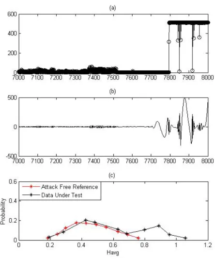
Figure 4.2 presents a case where attacks started around data point 7800. As can be observed from figure 4.2(c), the Havg vs. Probability distribution shifted to the right compared with the reference distribution, indicating the start of an attack in network traffic. Indeed,HW of data with attacks is 23.8944>HW th1, we conclude that attacks just began in the network traffic.
Figure 4.2: Weighted Self-similarity Example 1: Data With Attacks (a) Data Under Test (b) First IMF (c)Havgvs. Probability
Figure 4.3 shows a case where the data under test includes attacks only. As can be observed from figure 4.3(c), theHavgvs. Probabilitydistribution significantly shifted away from the reference. Again, HW of all attacks data is 25.9630>HW th1, we conclude that there are still attacks in the network traffic.
Figure 4.3: Weighted Self-similarity Example 1: All Attacks Data (a) Data Under Test (b) First IMF (c)Havgvs. Probability
Figure 4.4 shows a case when network traffic attacks stopped. As can be seen from figure 4.4(c), the Havg vs. Probability distribution of data under test is significantly narrower and completely shifted away from the attack free reference. This is an indication that the attacks have stopped. The HW of the data under test is 54.0850. As 54.0850 >HW th2, we conclude that the attacks are over.
Figure 4.4: Weighted Self-similarity Example 1: Attacks Stopped Data (a) Data Under Test (b) First IMF (c)Havgvs. Probability
More testing results are shown as follows: Figure 4.5 shows the normal data of sample points at [2001, 3000] and [37001, 38000]; Figure 4.6 shows data with attacks of sample points at [42501, 43500] and [148501, 149500].
HW =13.5088 HW =14.8722
Figure 4.5: Weighted Self-similarity Example 2: Normal Data (a) Data Under Test (b)Havg vs. Probability
HW =24.3820 HW =26.1997
Figure 4.6: Weighted Self-similarity Example 2: Data With Attacks (a) Data Under Test (b)Havg vs. Probability
Figure 4.7 shows all attacks data of sample points at [153001, 154000] and [184501, 185500]; Figure 4.8 shows attacks stopped data of sample points at [342501, 343500] and [490501, 491500] (Note: as automated test did not change the window size, Figure 4.8 is different from Figure 4.4).
HW =27.3815 HW =23.2611
Figure 4.7: Weighted Self-similarity Example 2: All Attacks Data (a) Data Under Test (b)Havg vs. Probability
HW =26.3518 HW =30.3625
Figure 4.8: Weighted Self-similarity Example 2: Attacks Stopped Data (a) Data Under Test (b)Havg vs. Probability
4.2.2 Pearson’s Distance Based on Marginal Spectrum
Ran test on kddcup.data 10 percent.gz dataset with Denial of Service (DoS) attacks. Set the window size at 200 data points (which is 400 seconds in time), as the total length of kddcup.data 10 percent.gz dataset is 494021 data points, so there will be 2469 windows for testing. Tested 2469 windows in total, and 2216 windows were correctly detected.
The detection rate for DoS attacks is: 2216
2469=89.75%
Figure 4.9 shows a case where no attacks occurred in the network traffic. As can be observed from the figure, the marginal spectrum of normal data almost overlaps with the attack free reference. The Pearson’s distance between “Data Under Test” and “Attack Free Reference” is 0.2804, and 0.2804<dth, the traffic is normal (wheredth is 0.5000).
Figure 4.10 shows a case where attacks occurred in the network traffic. As can be observed from the figure, the marginal spectrum of data with attacks has a peak between 0.2 and 0.3, and the shape is totally different with the attack free reference. The Pearson’s distance between “Data Under Test” and “Attack Free Reference” is 0.9529, and 0.9529 >dth, we conclude that there are attacks in the traffic (wheredthis 0.5000).
More testing results are shown as follows:
Pearson’s d=0.2510 Pearson’s d=0.2455
Figure 4.11: Marginal Spectrum Example 2: Normal Data
Pearson’s d=0.9219 Pearson’s d=0.9814
Pearson’s d=0.9604 Pearson’s d=0.9474
Figure 4.13: Marginal Spectrum Example 2: All Attacks Data
Pearson’s d=0.8431 Pearson’s d=0.9361
Figure 4.14: Marginal Spectrum Example 2: Attacks Stopped Data
4.2.3 Rate Change of Energy Density Level
Ran test on kddcup.data 10 percent.gz dataset with Denial of Service (DoS) attacks. Set the window size at 1000 data points (which is 2000 seconds in time), as the total length of kddcup.data 10 percent.gz dataset is 494021 data points, so there will be 987 windows for testing. Tested 987 windows in total, and 747 windows were correctly detected.
The detection rate for DoS attacks is: 747
987=75.68%
Figure 4.15 shows a case where no attacks occurred in the network traffic. As can be observed from the figure, the slopes ofm1andm2are not much different, and they follow
the same trend. The rate of energy change∆m=m1−m2 =0.6125−0.5859=0.0266, and 0.0266<mth(0.5000), the traffic is normal.
Figure 4.16 shows a case where attacks occurred in the network traffic. As can be observed from the figure, the slopes have a significant change between m2 and m1, and they do not follow the same trend any more. The rate of energy change ∆m=m1−m2= 2.1155−0.0006=2.1149, and 2.1149>mth(0.5000), we conclude that there are attacks in the traffic.
More testing results are shown as follows:
∆m=m2−m1=0.0643 ∆m=m2−m1=0.0435
Figure 4.17: Autocorrelation of Energy Density Level Example 2: Normal Data
∆m=m2−m1=2.1162 ∆m=m2−m1=1.6202
∆m=m2−m1=0.5037 ∆m=m2−m1=0.8439
Figure 4.19: Autocorrelation of Energy Density Level Example 2: All Attacks Data
∆m=m2−m1=0.9836 ∆m=m2−m1=0.5547
Figure 4.20: Autocorrelation of Energy Density Level Example 2: Attacks Stopped Data
CHAPTER 5: CONCLUSION AND FUTURE WORK
This thesis proposed three novel methods for network traffic anomaly detection based on three signal characteristics: the first IMF, marginal spectrum and energy density level. The weighted self-similarity parameter is calculated based on the first IMF and is introduced with the concept of entropy. Pearson’s distance is calculated based on the marginal spectrum to differentiate normal traffic from abnormal ones. And the rate change of energy density level is calculated based on the difference of slopes of autocorrelation.
Experimental test results on kddcup.data 10 percent.gz dataset with Denial of Ser-vice attacks show improved detection rates of network traffic anomaly – the weighted simi-larity parameter provides a 62.4% detection rate (without the “Neptune” in the DoS attacks, the detection rate was 78.62%): 616 out of 987 windows were correctly detected; the en-ergy density based detection provides a 75.7% detection rate: 747 out of 987 windows were correctly detected; and the Pearson’s distance yields an 89.8% detection rate: 2216 out of 2469 windows were correctly detected.
Future work includes: (1) Refine each method to future improve the detection rate. (2) Adjust the window size of each method and utilize a combination of the three param-eters, to achieve attack-specific, accurate, and timely detection. (3) Collect real-time data from a network to verify the robustness of the proposed detection methods.
[1] S. Papavassiliou, M. Pace, and L. Ho, “Implementing enhanced network maintenance for transaction access services: Tools and applications,” inIEEE International Confer-ence on Communications, vol. 1, pp. 211- 215, 2000.
[2] D. H. Kang, B. K. Kim, and J. T. Oh, “Protocol anomaly and pattern matching based intrusion detection system,” inWSEAS Transactions on Communication, vol.4, no. 10, pp. 994-1101, 2005.
[3] M. Thottan and J. Chuanyi, “Anomaly detection in IP networks,” in IEEE Trans. on Signal Processing, vol. 51, no. 8, pp. 2191-2204, 2003.
[4] L. Feinstein, and et al., “Statistical approaches to DDoS attack detection and response,” inProc., DARPA information survivability conference and exposition proceedings, vol. 1, pp. 303-314, 2003.
[5] M. Li, “An approach to reliably identifying signs of DDoS flood attacks based on LRD traffic pattern recognition,” inComputers & Security, vol. 23, pp. 549-558, 2004.
[6] M. H. Li, M. Li, and X. Y. Jiang, “DDoS attacks detection model and its application,” inWSEAS Transactions on Computers, Issue 8, vol. 7, pp. 1159-168, 2008.
[7] M. Li, “Change trend of averaged Hurst parameter of traffic under DDoS flood at-tacks,” in Computers & Security, vol. 25, no. 3, pp. 213-220, 2006.
[8] S. S. Kim, A. L. N. Reddy, and M. Vannucci, “Detecting traffic anomalies through aggregate analysis of packet header data,” in International IFIT-TC6 Networking Conference, Greece, vol. 3042, pp. 1047-1059, 2004.
[9] P. Abrey, R. Baraniuk, P. Flaudrin, R. Riedi, and D. Veitch, “Multiscale nature of network traffic,” inIEEE Signal Processing Magazine, pp. 28-46, 2002.
[10] X. Wang, L. Pang Q. Pei and X. Li, “A scheme for fast network traffic anomaly detection,” inComputer Application and System Modeling, Xi’an, China, pp. V1-592-V1-596, 2010.
[11] H. Jiang, L. pang, “Fast Network Traffic Anomaly Detection Based on Iteration,” Computational Intelligence and Security(CIS), 2011 Seventh International Conference, vol., no., pp.1006-1010, Dec 2011.
[12] Limthong, K.; Watanapongse, P.; Kensuke, F. “A wavelet-based anomaly detection for outbound network traffic,” in Information and Telecommunication Technologies (APSITT), pp.1-6, 15-18 June 2010.
[13] J. D. Brutlag, “Aberrant behavior detection in time series for network monitoring,” in LISA ’00: Proceedings of the 14th USENIX conference on System administration, Berkeley, CA, USA: USENIX Association, pp. 139-146, 2000.
[14] C.-M. Cheng, H. Kung, and K.-S. Tan, “Use of spectral analysis in defense against DoS attacks,” in Global Telecommunications Conference, 2002. GLOBECOM ’02. IEEE, vol. 3, pp. 2143-2148 vol.3, Nov. 2002.
[15] Y. Chen and K. Hwang, “Spectral analysis of tcp flows for defense against reduction-of-quality attacks,” in Communications, 2007. ICC ’07. IEEE International Confer-ence, pp. 1203-1210, June 2007.
[16] Y. Gu, A. McCallum, and D. Towsley, “Detecting anomalies in network traffic using maximum entropy estimation,” inIMC ’05: Proceedings of the 5th ACM SIGCOMM conference on Internet Measurement, Berkeley, CA, USA: USENIX Association, pp. 32-32, 2005.
[17] A. Wagner and B. Plattner, “Entropy based worm and anomaly detection in fast IP networks,” in Enabling Technologies: Infrastructure for Collaborative Enterprise, 2005. 14th IEEE International Workshops, pp. 172-177, June 2005.
[18] A. Lakhina, M. Crovella, and C. Diot, “Diagnosing network-wide traffic anomalies,” in SIGCOMM ’04: Proceedings of the 2004 conference on Applications, technolo-gies, architectures, and protocols for computer communications, New York, NY, USA: ACM, pp. 219-230, 2004.
[19] B. I. P. Rubinstein, B. Nelson, L. Huang, A. D. Joseph, S.-h. Lau, N. Taft and D. Tygar, “Compromising pca-based anomaly detectors for network-wide traffic,” EECS Department, University of California, Berkeley, Tech. Rep. UCB/EECS-2008-73, May 2008.
[20] H. Ringberg, A. Soule, J. Rexford, and C. Diot, “Sensitivity of pca for traffic anomaly detection,” inSIGMETRICS Perform. Eval. Rev., vol. 35, no. 1, pp. 109-120, 2007.
[21] V. Alarcon-Aquino and A. Barria, “Anomaly detection in communication networks using wavelets,” inIEEE Proc-Commun, vol. 148, no. 6, pp. 355-362, 2001.
[22] A. Ramanathan, “WADeS: A tool for distributed denial of service attack detection,” inTAMU-ECE-2002-02, Master of Science Thesis, Texas A& M University, 2002.
[23] P. Barford, J. Kline, D. Plonka, and A. Ron, “A signal analysis of traffic anomalies,” inIMW ’02 Proceedings of the 2nd ACM SIGCOMM Workshop on Internet measure-ment, pp. 71-82, 2002.
[24] S. S. Kim and A. Reddy, “Detecting traffic anomalies at the source through aggregate analysis of packet header data,” inProceedings of Networking, 2004.
[25] Li, L., Gyungho Lee, “DDos attack detection and wavelets,” in Computer Com-munications and Networks, 2003. ICCCN 2003. Proceedings. The 12th International Conference, pp.421-427, 20-22 Oct. 2003.
[26] K. Zheng, X. Wang, Y. Yang and S. Guo, “Detecting DDoS Attack With Hilbert-Huang Transformation,” in China Communications, Beijing, China, pp. 126-133, 2011.
[27] N.E. Huang, Z. Shen, S.R. Long, M.C. Wu, H.H. Shih, Q. Zheng, N. Yen, C.C. Tung, and H.H. Liu, “The empirical mode decomposition and the Hilbert spectrum for non-linear and non-stationary time series analysis,” Proc. Roy. Soc., London. A, vol.454, pp. 903-995, 1998.
[28] J. Z. Zhang, B. T. Price, R. D. Adams and T. J. Knaga, “Detection of Involuntary Hu-man Hand Motions Using Empirical Mode Decomposition and Hilbert-Huang Trans-form,” in Circuits and systems, MWSCAS 2008. 51st Midwest Symposium, pp. 157-160, Aug. 2008.
[29] M. S. Taqqu, V. Teverovsky and W. Willinger “Estimators for long-range dependence: an expirical study,” Fractals, vol. 3, no. 4, pp. 785-798, 1995.
[30] M. Tavallaee, E. Bagheri, W. Lu and A. Ghorbani, “A Detailed Analysis of the KDD CUP 99 Data Set,” in Computational Intelligence for Security and Defense Applica-tions, Ottawa, pp. 1-6, 2009.
[31] S. J. Stolfo, W. Fan, W. Lee, A. Prodromidis, and P. K. Chan, “Costbased modeling for fraud and intrusion detection: Results from the jam project,” DARPA Information Survivability Conference and Exposition, 2000. DISCEX ’00. Proceedings , vol. 02, pp. 130-144, 2000.
[32] R. P. Lippmann, D. J. Fried, I. Graf, J. W. Haines, K. R. Kendall, D. McClung, D. Weber, S. E. Webster, D. Wyschogrod, R. K. Cunningham, and M. A. Zissman, “Eval-uating intrusion detection systems: The 1998 darpa off-line intrusion detection evalu-ation,” DARPA Information Survivability Conference and Exposition, 2000. DISCEX ’00. Proceedings, vol. 02, pp. 12-26, 2000.
[33] MIT Lincoln Labs, 1998 DARPA Intrusion Detection Evaluation. Avail-able at: http://www.ll.mit.edu/mission/communications/ist/corpora/ideval/index.html, February 2008.
[34] KDD Cup 1999, Available at: http://kdd.ics.uci.edu/databases/kddcup99/task.html, Ocotber 2007.
[35] Kayacik, H. Gunes, A. Nur Zincir-Heywood, and Malcolm I. Heywood, “Selecting features for intrusion detection: A feature relevance analysis on KDD 99 intrusion de-tection datasets,” inProceedings of the Third Annual Conference on Privacy, Security and Trust (PST-2005), 2005.
[36] X. Cheng, K. Xie and D. Wang, “Network traffic anomaly detection based on self-similarity using HHT and wavelet transform,” in 5th International Conference on In-formation Assurance and Security, Baoding, China, pp. 710-713, 2009.
[37] John J. Shynk (2012). Probability, Random Variables, and Random Processes: The-ory and Signal Processing Applications. Wiley-Interscience.
APPENDIX A: TESTING RESULTS USING METHOD 1
Window size was 1000 sample points, the moving interval was 500 sample points, the total window number was 987. The detection criterion was: if HW ≤HW th1, set ‘c’ (Decision) = 1 (No Attacks); ifHW >HW th1, set ‘c’ (Decision) = 0 (With DoS Attacks). Test results are listed in the following table:
Column a: Window index number
Column b: HW (Weighted Self-similarity)
Column c: Decision (1: No Attacks; 0 With DoS Attacks) Column d: True/False (1: True; 0: False)
a b c d 1 17.95 1 1 2 17.32 1 1 3 13.11 1 1 4 16.77 1 1 5 13.51 1 1 6 15.50 1 1 7 20.06 0 0 8 21.70 0 0 9 24.90 0 0 10 18.94 1 1 11 17.29 1 1 12 17.04 1 1 13 13.46 1 1 14 14.99 1 1 15 23.51 0 1 16 28.22 0 1 17 25.04 0 1 18 25.72 0 1 19 31.92 0 1 20 31.15 0 1 21 25.08 0 1 22 25.62 0 1 23 24.48 0 1 24 28.08 0 0 25 15.23 1 1 26 22.17 0 0 27 15.87 1 1 28 14.67 1 1 29 19.73 1 1 30 24.33 0 0 31 31.13 0 1 32 26.64 0 1 33 29.72 0 0 34 22.52 0 0 35 17.54 1 1 36 15.85 1 1 37 21.51 0 0 38 26.13 0 1 39 27.05 0 1 40 23.41 0 0 41 15.51 1 1 42 13.78 1 1 43 16.25 1 1 44 24.10 0 0 45 21.61 0 0 46 24.77 0 0 47 22.12 0 0 48 14.55 1 1 49 15.64 1 1 50 15.70 1 1 51 17.29 1 1 52 17.89 1 1 53 18.86 1 1 54 24.41 0 0 55 21.92 0 0 56 17.33 1 1 57 14.45 1 1 58 16.63 1 1 59 19.62 1 1 60 18.31 1 1 61 18.70 1 1 62 16.59 1 1 63 15.31 1 0 64 16.12 1 0 65 17.36 1 1 66 15.55 1 1 67 15.48 1 1 68 14.33 1 1 69 15.34 1 1 70 20.76 0 0 71 24.33 0 0 72 21.05 0 0 73 17.37 1 1 74 17.17 1 1 75 14.87 1 1 76 15.86 1 1 77 16.14 1 1 78 17.69 1 1 79 17.60 1 0 80 20.55 0 1 81 22.86 0 1 82 19.68 1 0 83 22.65 0 0 84 22.43 0 0 85 23.03 0 0 86 24.38 0 1 87 24.92 0 1 88 22.03 0 1 89 26.68 0 1 90 27.26 0 1 91 31.37 0 1 92 28.41 0 1 93 19.06 1 0 94 25.36 0 1 95 27.85 0 1 96 24.34 0 1 97 21.93 0 1 98 27.73 0 1 99 22.15 0 1 100 24.26 0 1 101 21.44 0 1 102 26.34 0 1 103 19.44 1 0 104 19.26 1 0 105 24.63 0 0 106 21.08 0 0 107 25.73 0 1 108 24.07 0 1 109 23.34 0 1 110 21.14 0 1 111 21.57 0 1 112 15.10 1 0 113 14.29 1 0 114 15.82 1 0 115 20.29 0 1 116 18.90 1 0 117 16.09 1 0 118 17.55 1 0 119 19.60 1 0 120 16.98 1 0 121 18.74 1 0 122 17.88 1 0 123 15.65 1 0 124 21.53 0 1 125 18.54 1 0 126 11.24 1 0 127 18.16 1 0 128 20.70 0 1 129 20.61 0 1 130 12.70 1 0 131 11.18 1 0 132 11.79 1 0 133 12.05 1 0 134 13.76 1 0 135 15.83 1 0 136 9.49 1 0 137 8.98 1 0 138 12.21 1 0 139 11.58 1 0 140 9.98 1 0 141 10.57 1 0 142 14.36 1 0 143 14.58 1 0 144 10.06 1 0 145 9.05 1 0 146 13.87 1 0 147 15.10 1 0 148 18.40 1 0 149 22.19 0 1 150 24.64 0 0 151 26.52 0 0 152 26.42 0 1 153 26.32 0 1 154 21.39 0 0 155 16.15 1 1 156 22.92 0 1 157 17.04 1 0 158 18.75 1 0 159 12.22 1 1 160 16.02 1 1 161 19.99 1 1 162 18.41 1 1 163 19.49 1 1 164 17.07 1 1 165 19.75 1 0 166 19.11 1 0 167 16.00 1 1 168 16.20 1 1 169 15.76 1 1 170 15.86 1 1 171 18.02 1 1 172 20.91 0 0 173 24.67 0 1 174 27.06 0 1 175 15.27 1 1 176 24.41 0 0 177 16.44 1 1 178 15.66 1 1 179 21.99 0 0 180 22.88 0 0 181 25.40 0 0 182 24.91 0 0 183 27.40 0 0 184 26.44 0 1 185 23.09 0 1 186 29.87 0 1 187 18.08 1 0 188 28.76 0 1 189 25.57 0 1 190 23.19 0 1 191 20.26 0 1 192 20.65 0 1 193 28.17 0 1 194 28.85 0 1 195 27.98 0 1 196 30.69 0 1 197 37.87 0 1 198 27.28 0 1 199 22.02 0 1 200 23.58 0 1 201 24.44 0 1 202 28.56 0 1 203 26.54 0 1
204 30.79 0 1 205 25.12 0 1 206 37.69 0 1 207 26.40 0 1 208 28.54 0 1 209 15.82 1 1 210 14.13 1 1 211 17.56 1 1 212 19.77 1 1 213 17.07 1 1 214 15.86 1 1 215 21.87 0 0 216 20.35 0 1 217 17.03 1 0 218 14.91 1 0 219 13.69 1 0 220 14.18 1 0 221 14.95 1 0 222 14.68 1 0 223 11.98 1 0 224 20.73 0 1 225 16.53 1 0 226 14.37 1 0 227 15.16 1 0 228 20.30 0 1 229 17.92 1 0 230 17.33 1 0 231 14.84 1 0 232 14.52 1 0 233 13.20 1 0 234 14.69 1 0 235 16.06 1 0 236 18.05 1 0 237 16.62 1 0 238 14.11 1 0 239 15.95 1 0 240 14.46 1 0 241 9.94 1 0 242 12.25 1 0 243 15.61 1 0 244 7.97 1 0 245 15.34 1 0 246 8.10 1 0 247 14.27 1 0 248 7.82 1 0 249 10.82 1 0 250 6.21 1 0 251 12.85 1 0 252 6.60 1 0 253 6.99 1 0 254 11.17 1 0 255 14.77 1 0 256 19.85 1 0 257 20.37 0 1 258 30.60 0 1 259 28.37 0 1 260 24.18 0 1 261 26.71 0 1 262 31.08 0 1 263 25.98 0 1 264 23.34 0 1 265 22.41 0 1 266 29.28 0 1 267 24.73 0 1 268 24.61 0 1 269 21.55 0 1 270 28.01 0 1 271 31.25 0 1 272 24.45 0 1 273 24.32 0 1 274 30.00 0 1 275 27.85 0 0 276 16.91 1 1 277 15.88 1 1 278 15.09 1 1 279 16.29 1 1 280 21.07 0 1 281 17.99 1 0 282 24.33 0 0 283 27.23 0 1 284 23.76 0 1 285 18.21 1 0 286 25.44 0 1 287 31.23 0 1 288 20.99 0 0 289 21.02 0 0 290 19.01 1 1 291 30.73 0 0 292 22.37 0 0 293 19.90 1 1 294 20.17 0 0 295 19.38 1 1 296 20.11 0 0 297 20.87 0 0 298 26.20 0 1 299 20.86 0 1 300 24.18 0 1 301 23.85 0 1 302 21.71 0 1 303 22.48 0 1 304 23.24 0 1 305 20.31 0 1 306 20.91 0 1 307 27.38 0 1 308 25.14 0 1 309 21.67 0 1 310 26.66 0 1 311 27.68 0 1 312 22.27 0 1 313 25.34 0 1 314 22.62 0 1 315 23.17 0 1 316 23.46 0 1 317 31.11 0 1 318 27.17 0 1 319 24.09 0 1 320 18.02 1 0 321 16.18 1 0 322 19.94 1 0 323 24.98 0 1 324 25.08 0 1 325 18.09 1 0 326 24.59 0 1 327 27.04 0 1 328 19.25 1 0 329 22.63 0 1 330 21.58 0 1 331 24.01 0 1 332 24.22 0 1 333 22.05 0 1 334 22.65 0 1 335 24.21 0 1 336 26.12 0 1 337 29.45 0 1 338 25.74 0 1 339 19.88 1 0 340 22.65 0 1 341 22.50 0 1 342 22.97 0 1 343 23.25 0 1 344 29.05 0 1 345 27.64 0 1 346 25.36 0 1 347 22.88 0 1 348 27.59 0 1 349 23.22 0 1 350 27.22 0 1 351 29.49 0 1 352 21.94 0 1 353 22.90 0 1 354 20.82 0 1 355 29.65 0 1 356 23.86 0 1 357 25.57 0 1 358 31.89 0 1 359 27.31 0 1 360 27.36 0 1 361 20.54 0 1 362 28.71 0 1 363 22.95 0 1 364 31.10 0 1 365 28.29 0 1 366 25.12 0 1 367 24.02 0 1 368 31.94 0 1 369 28.16 0 1 370 23.26 0 1 371 27.29 0 1 372 24.07 0 1 373 21.48 0 1 374 32.45 0 1 375 22.73 0 1 376 25.75 0 1 377 20.53 0 1 378 21.89 0 1 379 20.62 0 1 380 23.42 0 1 381 25.62 0 1 382 24.01 0 1 383 23.86 0 1 384 20.96 0 1 385 19.58 1 0 386 28.52 0 1 387 20.54 0 1 388 27.21 0 1 389 28.09 0 1 390 21.22 0 1 391 20.03 0 1 392 23.15 0 1 393 19.06 1 0 394 17.63 1 0 395 18.11 1 0 396 19.37 1 0 397 17.55 1 0 398 19.83 1 0 399 22.71 0 1 400 18.12 1 0 401 20.24 0 1 402 16.51 1 0 403 20.71 0 1 404 22.29 0 1 405 22.53 0 1 406 22.09 0 1 407 19.69 1 0
408 17.17 1 0 409 15.32 1 0 410 16.45 1 0 411 15.55 1 0 412 18.28 1 0 413 21.37 0 1 414 18.55 1 0 415 16.29 1 0 416 15.69 1 0 417 17.05 1 0 418 20.74 0 1 419 19.84 1 0 420 18.26 1 0 421 16.48 1 0 422 21.66 0 1 423 21.15 0 1 424 21.98 0 1 425 25.15 0 1 426 25.49 0 1 427 18.05 1 0 428 17.14 1 0 429 19.43 1 0 430 16.70 1 0 431 20.14 0 1 432 20.29 0 1 433 21.20 0 1 434 19.73 1 0 435 18.06 1 0 436 22.09 0 1 437 20.35 0 1 438 21.52 0 1 439 20.72 0 1 440 21.78 0 1 441 22.48 0 1 442 20.30 0 1 443 17.48 1 0 444 17.57 1 0 445 21.64 0 1 446 20.82 0 1 447 18.73 1 0 448 19.93 1 0 449 23.53 0 1 450 19.38 1 0 451 16.95 1 0 452 28.49 0 1 453 20.86 0 1 454 17.83 1 0 455 20.75 0 1 456 18.67 1 0 457 24.45 0 1 458 19.10 1 0 459 16.03 1 0 460 18.27 1 0 461 18.91 1 0 462 18.83 1 0 463 20.70 0 1 464 22.85 0 1 465 23.19 0 1 466 19.66 1 0 467 20.16 0 1 468 18.40 1 0 469 19.97 1 0 470 23.77 0 1 471 18.65 1 0 472 18.22 1 0 473 19.19 1 0 474 18.46 1 0 475 19.43 1 0 476 19.49 1 0 477 17.91 1 0 478 15.90 1 0 479 15.36 1 0 480 17.89 1 0 481 17.83 1 0 482 18.16 1 0 483 22.99 0 1 484 20.54 0 1 485 22.37 0 1 486 24.95 0 1 487 22.36 0 1 488 20.40 0 1 489 16.98 1 0 490 16.20 1 0 491 21.55 0 1 492 23.20 0 1 493 18.18 1 0 494 19.32 1 0 495 20.10 0 1 496 20.31 0 1 497 23.12 0 1 498 19.60 1 0 499 20.01 0 1 500 18.76 1 0 501 18.32 1 0 502 21.89 0 1 503 18.19 1 0 504 22.10 0 1 505 13.99 1 0 506 21.01 0 1 507 24.42 0 1 508 26.55 0 1 509 16.48 1 0 510 23.76 0 1 511 21.31 0 1 512 19.35 1 0 513 18.10 1 0 514 22.55 0 1 515 21.98 0 1 516 20.66 0 1 517 23.81 0 1 518 28.53 0 1 519 20.98 0 1 520 20.22 0 1 521 23.72 0 1 522 21.36 0 1 523 15.31 1 0 524 21.14 0 1 525 22.81 0 1 526 25.11 0 1 527 29.10 0 1 528 26.97 0 1 529 20.55 0 1 530 22.74 0 1 531 24.69 0 1 532 21.75 0 1 533 29.01 0 1 534 23.70 0 1 535 27.11 0 1 536 33.06 0 1 537 22.20 0 1 538 19.83 1 0 539 21.37 0 1 540 23.54 0 1 541 25.63 0 1 542 21.13 0 1 543 28.04 0 1 544 18.48 1 0 545 22.53 0 1 546 26.91 0 1 547 28.12 0 1 548 25.06 0 1 549 23.21 0 1 550 20.67 0 1 551 21.46 0 1 552 22.12 0 1 553 19.36 1 0 554 29.31 0 1 555 25.90 0 1 556 25.73 0 1 557 25.08 0 1 558 34.57 0 1 559 23.75 0 1 560 22.44 0 1 561 28.40 0 1 562 23.76 0 1 563 26.87 0 1 564 22.06 0 1 565 21.56 0 1 566 19.23 1 0 567 26.56 0 1 568 25.36 0 1 569 28.03 0 1 570 35.95 0 1 571 30.87 0 1 572 20.21 0 1 573 24.39 0 1 574 26.58 0 1 575 25.80 0 1 576 22.34 0 1 577 21.94 0 1 578 21.91 0 1 579 25.25 0 1 580 24.73 0 1 581 23.29 0 1 582 23.64 0 1 583 32.30 0 1 584 26.64 0 1 585 23.56 0 1 586 29.20 0 1 587 27.39 0 1 588 17.56 1 0 589 20.92 0 1 590 27.77 0 1 591 24.11 0 1 592 23.42 0 1 593 20.11 0 1 594 22.87 0 1 595 22.38 0 1 596 21.30 0 1 597 19.94 1 0 598 29.23 0 1 599 21.78 0 1 600 27.86 0 1 601 24.62 0 1 602 25.62 0 1 603 21.04 0 1 604 18.47 1 0 605 26.11 0 1 606 25.35 0 1 607 20.24 0 1 608 24.56 0 1 609 25.56 0 1 610 27.11 0 1 611 28.11 0 1
612 20.15 0 1 613 23.96 0 1 614 30.11 0 1 615 26.51 0 1 616 24.16 0 1 617 23.93 0 1 618 22.33 0 1 619 29.37 0 1 620 27.32 0 1 621 31.61 0 1 622 24.06 0 1 623 20.12 0 1 624 26.66 0 1 625 20.16 0 1 626 19.01 1 0 627 23.69 0 1 628 25.06 0 1 629 31.41 0 1 630 28.24 0 1 631 23.93 0 1 632 20.25 0 1 633 26.98 0 1 634 18.01 1 0 635 29.85 0 1 636 22.43 0 1 637 23.37 0 1 638 24.04 0 1 639 20.04 0 1 640 23.95 0 1 641 27.31 0 1 642 30.49 0 1 643 27.42 0 1 644 22.96 0 1 645 24.49 0 1 646 24.71 0 1 647 26.31 0 1 648 26.27 0 1 649 28.81 0 1 650 28.72 0 1 651 20.75 0 1 652 26.82 0 1 653 24.00 0 1 654 28.15 0 1 655 28.29 0 1 656 37.07 0 1 657 28.14 0 1 658 23.50 0 1 659 29.42 0 1 660 22.94 0 1 661 23.30 0 1 662 24.36 0 1 663 19.35 1 0 664 33.85 0 1 665 19.94 1 0 666 20.50 0 1 667 23.84 0 1 668 27.68 0 1 669 23.65 0 1 670 23.70 0 1 671 17.46 1 0 672 27.26 0 1 673 20.42 0 1 674 26.24 0 1 675 27.73 0 1 676 27.71 0 1 677 23.95 0 1 678 22.56 0 1 679 27.63 0 1 680 23.87 0 1 681 18.19 1 0 682 20.72 0 1 683 29.73 0 1 684 23.34 0 1 685 23.37 0 1 686 26.35 0 1 687 20.99 0 0 688 21.14 0 0 689 27.96 0 1 690 22.01 0 1 691 19.50 1 0 692 24.71 0 1 693 25.33 0 1 694 25.85 0 1 695 32.99 0 0 696 30.41 0 0 697 24.31 0 0 698 24.40 0 1 699 18.99 1 0 700 18.36 1 0 701 20.39 0 1 702 16.27 1 0 703 15.48 1 0 704 16.03 1 0 705 15.32 1 0 706 14.49 1 0 707 23.04 0 1 708 18.03 1 0 709 29.24 0 1 710 20.74 0 1 711 17.40 1 0 712 17.13 1 0 713 19.28 1 0 714 15.37 1 0 715 17.04 1 0 716 15.02 1 0 717 16.90 1 0 718 18.14 1 0 719 21.07 0 1 720 17.85 1 0 721 16.78 1 0 722 17.40 1 0 723 15.84 1 0 724 18.13 1 0 725 20.68 0 1 726 17.45 1 0 727 19.52 1 0 728 13.79 1 0 729 13.49 1 0 730 14.92 1 0 731 13.76 1 0 732 22.17 0 1 733 21.19 0 1 734 17.91 1 0 735 17.26 1 0 736 18.57 1 0 737 17.03 1 0 738 15.88 1 0 739 15.59 1 0 740 23.37 0 1 741 25.62 0 1 742 28.50 0 1 743 28.67 0 1 744 25.07 0 1 745 26.11 0 1 746 9.30 1 0 747 6.35 1 0 748 7.08 1 0 749 11.28 1 0 750 9.31 1 0 751 14.05 1 0 752 5.25 1 0 753 8.53 1 0 754 13.22 1 0 755 10.40 1 0 756 14.37 1 0 757 9.63 1 0 758 9.90 1 0 759 9.80 1 0 760 15.48 1 0 761 15.91 1 0 762 10.86 1 0 763 8.94 1 0 764 7.73 1 0 765 7.25 1 0 766 6.70 1 0 767 11.88 1 0 768 13.24 1 0 769 12.35 1 0 770 4.39 1 0 771 6.50 1 0 772 16.08 1 0 773 19.70 1 0 774 24.31 0 1 775 21.64 0 1 776 16.33 1 0 777 11.75 1 0 778 18.46 1 0 779 15.47 1 0 780 5.51 1 0 781 11.94 1 0 782 14.26 1 0 783 17.01 1 0 784 13.50 1 0 785 6.08 1 0 786 7.45 1 0 787 8.86 1 0 788 9.14 1 0 789 13.69 1 0 790 10.14 1 0 791 6.76 1 0 792 4.53 1 0 793 16.51 1 0 794 23.10 0 1 795 27.67 0 1 796 23.72 0 1 797 25.78 0 1 798 20.40 0 1 799 25.55 0 1 800 23.40 0 1 801 19.79 1 0 802 20.96 0 1 803 22.32 0 1 804 22.07 0 1 805 20.84 0 1 806 27.79 0 1 807 28.53 0 1 808 24.37 0 1 809 24.93 0 1 810 22.49 0 1 811 22.35 0 1 812 19.28 1 0 813 20.18 0 1 814 21.73 0 1 815 19.37 1 0
816 21.72 0 1 817 19.03 1 0 818 21.07 0 1 819 19.91 1 0 820 23.23 0 1 821 21.25 0 1 822 24.42 0 1 823 16.62 1 0 824 31.76 0 1 825 24.35 0 1 826 18.42 1 0 827 17.12 1 0 828 16.07 1 0 829 14.39 1 0 830 14.41 1 0 831 16.78 1 0 832 16.05 1 0 833 20.95 0 1 834 23.44 0 1 835 27.99 0 1 836 24.99 0 1 837 23.39 0 1 838 33.27 0 1 839 32.08 0 1 840 34.23 0 1 841 37.07 0 1 842 36.75 0 1 843 33.04 0 1 844 34.13 0 1 845 27.59 0 1 846 35.06 0 1 847 25.77 0 1 848 26.84 0 1 849 36.85 0 1 850 25.81 0 1 851 22.62 0 1 852 26.12 0 1 853 23.47 0 1 854 25.99 0 1 855 21.20 0 1 856 21.61 0 1 857 22.55 0 1 858 24.13 0 1 859 26.82 0 1 860 29.73 0 1 861 37.49 0 1 862 33.75 0 1 863 27.83 0 1 864 29.00 0 1 865 37.71 0 1 866 42.53 0 1 867 34.24 0 1 868 41.59 0 1 869 26.74 0 1 870 31.23 0 1 871 25.20 0 1 872 31.13 0 1 873 30.90 0 1 874 39.45 0 1 875 40.09 0 1 876 28.60 0 1 877 30.87 0 1 878 26.60 0 1 879 29.90 0 1 880 21.07 0 1 881 21.60 0 1 882 21.51 0 1 883 22.51 0 1 884 24.08 0 1 885 25.39 0 1 886 24.73 0 1 887 23.82 0 1 888 22.64 0 1 889 29.36 0 1 890 25.01 0 1 891 37.45 0 1 892 21.89 0 1 893 25.09 0 1 894 25.79 0 1 895 37.69 0 1 896 25.10 0 1 897 25.37 0 1 898 25.48 0 1 899 21.33 0 1 900 25.50 0 1 901 18.62 1 1 902 23.75 0 0 903 21.34 0 0 904 27.66 0 1 905 23.43 0 1 906 26.06 0 0 907 24.04 0 0 908 22.37 0 0 909 21.88 0 0 910 30.94 0 0 911 18.48 1 0 912 18.37 1 0 913 23.11 0 1 914 20.66 0 0 915 18.89 1 1 916 19.77 1 1 917 24.63 0 1 918 20.31 0 1 919 14.94 1 0 920 17.14 1 0 921 21.37 0 1 922 13.35 1 0 923 14.04 1 0 924 15.68 1 0 925 17.46 1 0 926 15.97 1 0 927 15.31 1 0 928 11.08 1 0 929 14.07 1 0 930 17.31 1 0 931 17.36 1 0 932 18.18 1 0 933 17.93 1 0 934 19.69 1 0 935 16.08 1 0 936 14.86 1 0 937 17.84 1 0 938 13.73 1 0 939 14.31 1 0 940 24.67 0 1 941 18.27 1 0 942 14.12 1 0 943 16.02 1 0 944 15.00 1 0 945 11.69 1 0 946 14.25 1 0 947 15.80 1 0 948 7.79 1 0 949 7.60 1 0 950 7.41 1 0 951 13.20 1 0 952 4.89 1 0 953 12.07 1 0 954 7.08 1 0 955 13.32 1 0 956 9.99 1 0 957 12.72 1 0 958 6.74 1 0 959 13.25 1 0 960 32.03 0 1 961 23.39 0 1 962 20.22 0 1 963 19.15 1 1 964 19.40 1 1 965 16.95 1 1 966 15.16 1 1 967 15.48 1 1 968 16.59 1 1 969 13.53 1 1 970 14.37 1 0 971 15.75 1 0 972 14.28 1 0 973 18.56 1 0 974 31.38 0 1 975 25.38 0 1 976 21.65 0 1 977 29.10 0 1 978 19.76 1 0 979 27.72 0 1 980 22.19 0 1 981 26.59 0 1 982 30.36 0 1 983 23.96 0 0 984 25.79 0 0 985 16.46 1 1 986 11.43 1 1 987 13.26 1 1
APPENDIX B: TESTING RESULTS USING METHOD 2
Window size was 200 sample points, the moving interval was 200 sample points, the total window number was 2469. The detection criterion was: ifd ≤dth, set ‘c’ (Deci-sion) = 1 (No Attacks); ifd>dth, set ‘c’ (Decision) = 0 (With DoS Attacks). Test results are listed in the following table:
Column a: Window index number Column b: Pearson’s Distance ‘d’
Column c: Decision (1: No Attacks; 0 With DoS Attacks) Column d: True/False (1: True; 0: False)