6-15-2017
A Nonconvex Splitting Method for Symmetric
Nonnegative Matrix Factorization: Convergence
Analysis and Optimality
Songtao Lu
Iowa State University, [email protected]
Mingyi Hong
Iowa State UniversityZhengdao Wang
Iowa State University, [email protected]
Follow this and additional works at:
http://lib.dr.iastate.edu/ece_pubs
Part of the
Industrial Technology Commons
, and the
Signal Processing Commons
The complete bibliographic information for this item can be found at
http://lib.dr.iastate.edu/
ece_pubs/162
. For information on how to cite this item, please visit
http://lib.dr.iastate.edu/
howtocite.html
.
This Article is brought to you for free and open access by the Electrical and Computer Engineering at Iowa State University Digital Repository. It has been accepted for inclusion in Electrical and Computer Engineering Publications by an authorized administrator of Iowa State University Digital Repository. For more information, please [email protected].
Factorization: Convergence Analysis and Optimality
Abstract
Symmetric nonnegative matrix factorization (SymNMF) has important applications in data analytics
problems such as document clustering, community detection, and image segmentation. In this paper, we
propose a novel nonconvex variable splitting method for solving SymNMF. The proposed algorithm is
guaranteed to converge to the set of Karush-Kuhn-Tucker (KKT) points of the nonconvex SymNMF
problem. Furthermore, it achieves a global sublinear convergence rate. We also show that the algorithm can be
efficiently implemented in parallel. Further, sufficient conditions are provided that guarantee the global and
local optimality of the obtained solutions. Extensive numerical results performed on both synthetic and real
datasets suggest that the proposed algorithm converges quickly to a local minimum solution.
Keywords
Symmetric nonnegative matrix factorization, Karush-Kuhn-Tucker points, variable splitting, global and local
optimality, clustering
Disciplines
Electrical and Computer Engineering | Industrial Technology | Signal Processing
CommentsThis is a manuscript of an article published as Lu, Songtao, Mingyi Hong, and Zhengdao Wang. "A nonconvex
splitting method for symmetric nonnegative matrix factorization: Convergence analysis and optimality." IEEE
Transactions on Signal Processing (2017). DOI:
10.1109/TSP.2017.2679687
. Posted with permission.
Rights© 2017 IEEE. Personal use of this material is permitted. Permission from IEEE must be obtained for all other
uses, in any current or future media, including reprinting/republishing this material for advertising or
promotional purposes, creating new collective works, for resale or redistribution to servers or lists, or reuse of
any copyrighted component of this work in other works.
arXiv:1703.08267v1 [math.OC] 24 Mar 2017
A Nonconvex Splitting Method for Symmetric
Nonnegative Matrix Factorization:
Convergence Analysis and Optimality
Songtao Lu,
Student Member, IEEE
, Mingyi Hong,
Member, IEEE
and Zhengdao Wang,
Fellow, IEEE
Abstract—Symmetric nonnegative matrix factorization
(SymNMF) has important applications in data analytics
problems such as document clustering, community detection and image segmentation. In this paper, we propose a novel nonconvex variable splitting method for solving SymNMF. The proposed algorithm is guaranteed to converge to the set of Karush-Kuhn-Tucker (KKT) points of the nonconvex SymNMF problem. Furthermore, it achieves a global sublinear convergence rate. We also show that the algorithm can be efficiently implemented in parallel. Further, sufficient conditions are provided which guarantee the global and local optimality of the obtained solutions. Extensive numerical results performed on both synthetic and real data sets suggest that the proposed algorithm converges quickly to a local minimum solution.
Index Terms—Symmetric nonnegative matrix factorization, Karush-Kuhn-Tucker points, variable splitting, global and local optimality, clustering
I. INTRODUCTION
Nonnegative matrix factorization (NMF) refers to factoring a given matrix into the product of two matrices whose entries are all nonnegative. It has long been recognized as an important matrix decomposition problem [1], [2]. The requirement that the factors are component-wise nonnegative makes NMF distinct from traditional methods such as the principal component analysis (PCA) and the linear discriminant analysis (LDA), leading to many interesting applications in imaging, signal processing and machine learning [3]–[7]; see [8] for a recent survey. When further requiring that the two factors are identical after transposition, NMF becomes the so-called symmetric nonnegative matrix factorization (SymNMF). In the case where the given matrix cannot be factorized exactly, an approximate solution with a suitably defined approximation error is desired. Mathematically, SymNMF approximates a given (usually symmetric) nonnegative matrix Z ∈ RN×N by a low rank
Manuscript received May 15, 2016; revised October 6, 2016, January 6, 2017, and February 16, 2017; accepted February 20, 2017. The associate editor coordinating the review of this manuscript and approving it for publication was Marco Moretti. Part of the paper was presented at the 42nd IEEE International Conference on Acoustics, Speech, and Signal Processing (ICASSP), New Orleans, March 5–9, 2017. This work was supported in part by NSF under Grants No. 1523374 and No. 1526078, and by AFOSR under Grant No. 15RT0767.
Songtao Lu and Zhengdao Wang are with the Department of Electrical and Computer Engineering, Iowa State University, Ames, IA 50011, USA (emails:
{songtao, zhengdao}@iastate.edu).
Mingyi Hong is with the Department of Industrial and Manufacturing Systems Engineering, Iowa State University, Ames, IA 50011, USA (email: [email protected]).
matrix XXT
, where the factor matrix X ∈ RN×K is
component-wise nonnegative, typically with K ≪ N. Let
k · kF denote the Frobenius norm. The problem can be
formulated as a nonconvex optimization problem [9]–[11]:
min X≥0 f(X) = 1 2kXX T −Zk2F. (1) Recently, SymNMF has found many applications in document clustering, community detection, image segmentation and pattern clustering in bioinformatics [9], [11], [12]. An important class of clustering methods is known as spectral clustering, e.g., [13], [14], which is based on the eigenvalue decomposition of some transformed graph Laplacian matrix. In [15], it has been shown that spectral clustering and SymNMF are two different ways of relaxing the kernel K-means clustering, where the former relaxes the nonnegativity constraint while the latter relaxes certain orthogonality constraint. SymNMF also has the advantage of often yielding more meaningful and interpretable results [11].
A. Related Work
Due to the importance of the NMF problem, many algorithms have been proposed in the literature for finding its high-quality solutions. Well-known algorithms include the multiplicative update [6], alternating projected gradient methods [16], alternating nonnegative least squares (ANLS) with the active set method [17] and a few recent methods such as the bilinear generalized approximate message passing [18], [19], as well as methods based on the block coordinate descent [20]. These methods often possess strong convergence guarantees (to Karush-Kuhn-Tucker (KKT) points of the NMF problem) and most of them lead to satisfactory performance in practice; see [8] and the references therein for detailed comparison and comments for different algorithms. Unfortunately, most of the aforementioned methods for NMF lack effective mechanisms to enforce the symmetry between the resulting factors, therefore they are not directly applicable to SymNMF. Recently, there have been works focusing on customized algorithms for SymNMF, which we review below.
To this end, first rewrite SymNMF equivalently as
min Y≥0,X=Y 1 2kXY T −Zk2F. (2)
A simple strategy is to ignore the equality constraintX=Y, and then alternatingly perform the following two steps: 1) solving Y with X being fixed (a nonnegative least squares
problem); 2) solving X with Y being fixed (a least squares problem). Such ANLS algorithm has been proposed in [11] for dealing with SymNMF. Unfortunately, despite the fact that an optimal solution can be obtained in each subproblem, there is no guarantee that theY-iterate will converge to theX-iterate. The algorithm in [11] adds a regularized term for the difference between the two factors to the objective function and explicitly enforces that the two matrices are equal at the output. Such an extra step enforces symmetry, but unfortunately also leads to the loss of global convergence guarantees. A related ANLS-based method has been introduced in [10]; however the algorithm is based on the assumption that there exists an exact symmetric factorization (i.e., ∃ X≥0 such that XXT =Z
). Without such assumption, the algorithm may not converge to the set of KKT points1of problem (1). A multiplicative update
for SymNMF has been proposed in [9], but the algorithm lacks convergence guarantees (to KKT points of problem (1)) [21], and has a much slower convergence speed than the one proposed in [10]. In [11], [22], algorithms based on the projected gradient descent (PGD) and the projected Newton (PNewton) have been proposed, both of which directly solve the original formulation (1). Again there has been no global convergence analysis since the objective function is a nonconvex fourth-order polynomial. More recently, the work [23] applies the nonconvex coordinate descent (CD) algorithm for SymNMF. Due to the fact that the minimizer of the fourth order polynomial is not unique in each coordinate updating, the CD-based method may not converge to stationary points.
Another popular method for NMF is based on the alternating direction method of multipliers (ADMM), which is a flexible tool for large scale convex optimization [24]. For example, using ADMM for both NMF and matrix completion, high quality results have been obtained in [25] for gray-scale and hyperspectral image recovery. Furthermore, ADMM has been applied to generalized versions of NMF where the objective function is the general beta-divergence [26]. A hybrid alternating optimization and ADMM method was proposed for NMF, as well as tensor factorization, under a variety of constraints and loss measures in [27]. However, despite the promising numerical results, none of the works discussed above has rigorous theoretical justification for SymNMF. Recently, the work [28] has applied the ADMM for NMF and provided one of the first analysis for using ADMM to solve nonconvex matrix-factorization type problems. However, it is important to note that the algorithm in [28] does not apply to the SymNMF case, because our problem is more restrictive in that symmetric factors are desired, while in NMF symmetry is not enforced. Technically, imposing symmetry poses much difficulty in the analysis (we will comment on this point shortly). In fact, the convergence of ADMM for SymNMF is still open in the literature.
An important research question for NMF and SymNMF is whether it is possible to design algorithms that lead toglobally
optimal solutions. At the first sight such problem appears very challenging since finding the exact NMF is NP-hard
1Letd(a, s)denote the distance between two pointsaands. We say that
a sequenceaiconverges to a setSif the distance betweenaiandS, defined
asinfs∈Sd(ai, s), converges to zero, asi→ ∞.
[29] and checking whether a positive semidefinite matrix can be decomposed exactly by SymNMF is also NP-hard [30]. However, some promising recent findings suggest that when the structure of the underlying factors are appropriately utilized, it is possible to obtain rather strong results. For example, in [31], the authors have shown that for the low rank factorized stochastic optimization problem where the two low rank matrices are symmetric, a modified stochastic gradient descent algorithm is capable of converging to a global optimum with constant probability from a random starting point. Related works also include [32]–[34]. However, when the factors are required to be nonnegative and symmetric, it is no longer clear whether the existing analysis can still be used to show convergence to global/local optimal points. For the nonnegative principal component problem (i.e., finding the leading nonnegative eigenvector) under the spiked model, reference [35] shows that certain approximate message passing algorithm is able to find the global optimal solution asymptotically. Unfortunately, this analysis does not generalize to an arbitrary symmetric observation matrix for the case
K > 1. To our best knowledge, a characterization of global and local optimal solutions for SymNMF is still lacking.
B. Contributions
In this paper, we first propose a novel algorithm for SymNMF, which utilizes nonconvex splitting and is capable of converging to the set of KKT points with a provable global convergence rate. The main idea is to relax the symmetry requirement at the beginning and gradually enforce it as the algorithm proceeds. Second, we provide a number of easy-to-check sufficient conditions guaranteeing the local or global optimality of the obtained solutions. Numerical results on both synthetic and real data show that the proposed algorithm achieves fast and stable convergence (often to local minimum solutions) with low computational complexity.
More specifically, the main contributions of this paper are: 1) We design a novel nonconvex splitting SymNMF (NS-SymNMF) algorithm, which converges to the set of KKT points of SymNMF with a global sublinear rate. To our best knowledge, it is the first SymNMF solver that possesses global convergence rate guarantees.
2) We provide a set of easily checkable sufficient conditions (which only involve finding the smallest eigenvalue of certain matrix) that characterize the global and local optimality of the solutions. By utilizing such conditions, we demonstrate numerically that with high probability, our proposed algorithm converges not only to the set of KKT points but to a local optimal solution as well.
Notation:Bold upper case letters without subscripts (e.g.,
X,Y) denote matrices and bold lower case letters without subscripts (e.g., x,y) represent vectors. The notation Zi,j
denotes the (i, j)-th entry of matrix Z. Vector Xi denotes
theith row of matrixX andX′
m denotes themth column of
the matrix.
II. THEPROPOSEDALGORITHM
The proposed algorithm leverages the reformulation (2). Our main idea is to gradually tighten the difficult equality
constraint X = Y as the algorithm proceeds so that when convergence is approached, such equality is eventually satisfied. To this end, let us construct the augmented Lagrangian for (2), given by
L(X,Y;Λ) = 1 2kXY T −Zk2F+hY−X,Λi+ρ 2kY−Xk 2 F (3) where Λ∈ RN×K is a matrix of dual variables, h·idenotes
the inner product operator, and ρ >0 is a penalty parameter whose value will be determined later.
It may be tempting to directly apply the well-known ADMM method to the augmented Lagrangian (3), which alternatingly minimizes the primal variablesXandY, followed by a dual ascent stepΛ←Λ+ρ(Y−X). Unfortunately, the classical result for ADMM presented in [24], [36], [37] only works for convex problems, hence they do not apply to our nonconvex problem (2) (note this is a linearly constrained nonconvex
problem where the nonconvexity arises in the objective function). Recent results such as [38]–[41] that analyze ADMM for nonconvex problems do not apply either, because in these works the basic requirements are: 1) the objective function is separable over the block variables; 2) the smooth part of the augmented Lagrangian has Lipschitz continuous gradient with respect to all variable blocks. Unfortunately neither of these conditions are satisfied in our problem.
Next we begin presenting the proposed algorithm. We start by considering the following reformulation of problem (1)
min X,Y 1 2kXY T −Zk2F (4) s.t. Y≥0, X=Y, kYik22≤τ, ∀ i,
whereτ >0 is some given constant.
Let Ω∗ denote the dual matrix for the constraint X ≥ 0
in the Lagrangian of problem (1). The KKT conditions of problem (1) are given by [42, eq. (5.49)]
2 X∗(X∗)T −Z T+Z 2 X∗−Ω∗= 0, (5a) Ω∗≥0, (5b) X∗≥0, (5c) X∗◦Ω∗=0 (5d) where ◦ denotes the Hadamard product. For a point X∗, if we can find some Ω∗ such that (X∗,Ω∗)satisfies conditions (5a)–(5d), then we term X∗ aKKT point of problem (1).
A stationary point for problem (1) is a point X∗
that satisfies the following optimality condition [43, Proposition 2.1.2]: X∗(X∗)T −Z T +Z 2 X∗,X−X∗ ≥0, ∀X≥0. (6) It can be checked that when τ in (4) is sufficiently large (larger than a threshold dependent on Z), then problem (4) is
equivalentto problem (1), in the sense that the KKT pointsX∗
of the two problems are identical. Also, there is a one-to-one correspondence between the KKT points and stationary points of the SymNMF problem, although in general such one-to-one correspondence may not hold. To be more precise, we have:
Lemma 1. For problem (1), a point X∗, is a KKT point,
which means there exists someΩ∗such that(X∗,Ω∗)satisfies
(5a)–(5d), if and only ifX∗is a stationary point, which means
it satisfies(6).
Proof:See Section VII-A
Lemma 2. Supposeτ > θk,∀kwhere
θk ,
Zk,k+12qPNi=1(Zi,k+Zk,i)2
2 , (7)
then the KKT points of problem (1) and the KKT points of
problem(4) have a one-to-one correspondence.
Proof:See Section VII-B.
We remark that the previous work [23] has made the observation that solving SymNMF with the additional constraints kXik2 ≤
p
2kZkF,∀i will not result in any loss
of theglobaloptimality. Lemma 2 provides a stronger result, that allKKTpoints of SymNMF are preserved within asmaller
bounded feasible set Y , {Y | Yi ≥ 0,kYik2
2 ≤ τ,∀i}
(note, thatτ ≪2kZkF in general).
The proposed NS-SymNMF algorithm alternates between the primal updates of variablesXandY, and the dual update for Λ. Below we present its detailed steps (superscript t is used to denote the iteration number).
Y(t+1)= arg min Y≥0,kYik2 2≤τ,∀i 1 2kX (t)YT −Zk2F +ρ 2kY−X (t)+Λ(t)/ρ k2F+ β(t) 2 kY−Y (t) k2F, (8) X(t+1)= arg min X 1 2kX(Y (t+1))T −Zk2F +ρ 2kX−Λ (t)/ρ −Y(t+1)k2F, (9) Λ(t+1)=Λ(t)+ρ(Y(t+1)−X(t+1)), (10) β(t+1)=6 ρkX (t+1)(Y(t+1))T −Zk2F. (11)
We remark that this algorithm is very close in form to the standard ADMM method applied to problem (4) (which lacks convergence guarantees). The key difference is the use of the proximal term kY−Y(t)k2F multiplied by an iteration
dependent penalty parameter β(t) ≥ 0, whose value is
proportional to the size of the objective value. Intuitively, if the algorithm converges to a solution with a small objective value, then parameter β(t) vanishes in the limit. Introducing such
proximal term is one of the main novelty of the algorithm, and it is crucial in guaranteeing the convergence of NS-SymNMF.
III. CONVERGENCEANALYSIS
In this section we provide convergence analysis of NS-SymNMF for a general SymNMF problem. We do not require Z to be symmetric, positive-semidefinite, or to have positive entries. We assumeK can be any integer in[1, N].
A. Convergence and Convergence Rate
Below we present our first main result, which asserts that when the penalty parameter ρ is sufficiently large, the NS-SymNMF algorithm converges globally to the set of KKT points of problem (1).
Theorem 1. Suppose the following is satisfied
ρ >6N τ. (12)
Then the following statements are true for NS-SymNMF:
1) The equality constraint is satisfied in the limit, i.e.,
lim t→∞kX
(t)
−Y(t)k2F →0.
2) The sequence {X(t),Y(t)Λ(t)} generated by the
algorithm is bounded. And every limit point of the
sequence is a KKT point of problem(1).
An equivalent statement on the convergence is that the sequence{X(t),Y(t)Λ(t)}converges to the set of KKT points of problem (1); cf. footnote 1 on Page 2.
Proof: See Section VII-C.
Our second result characterizes the convergence rate of the algorithm. To this end, we construct a function that measures the optimality of the iterates {X(t),Y(t),Λ(t)}. Define the
proximal gradient of the augmented Lagrangian function as
e ∇L(X,Y,Λ), YT −proj Y[YT− ∇Y(L(Y,X,Λ)] ∇XL(X,Y,Λ) where
projY(W),arg min
Y≥0,kYik2 2≤τ,∀i
kW−Yk2F (13) i.e., it is the projection operator that projects a given matrix
W onto the feasible set of Y. Here we propose to use the following quantity to measure the progress of the algorithm
P(X(t),Y(t),Λ(t)),k∇Le (X(t),Y(t),Λ(t))k2F
+kX(t)−Y(t)k2F. (14) It can be verified that iflimt→∞P(X(t),Y(t),Λ(t)) = 0, then
a KKT point of problem (1) is obtained.
Below we show that the functionP(X(t),Y(t),Λ(t)) goes to zero in a sublinear manner.
Theorem 2. For a given small constantǫ, letT(ǫ)denote the iteration index satisfying the following inequality
T(ǫ),min{t| P(X(t),Y(t),Λ(t))≤ǫ, t≥0}. (15)
Then there exists some constant C >0such that
ǫ≤ CL(X
(1),Y(1),Λ(1))
T(ǫ) . (16)
Proof: See Section VII-D.
The result indicates that it takes O(1/ǫ) iterations for P(X(t),Y(t),Λ(t)) to be less than ǫ. It follows that NS-SymNMF converges sublinearly.
B. Sufficient Global and Local Optimality Conditions
Since problem (1) is not convex, the KKT points obtained by NS-SymNMF could be different from the global optimal solutions. Therefore it is important to characterize the conditions under which these two different types of solutions coincide. Below we provide an easily checkable sufficient condition to ensure that a KKT point X∗ is also a globally optimal solution for problem (1).
Theorem 3. Suppose thatX∗ is a KKT point of problem(1).
Then, X∗ is also a global optimal point if the following is
satisfied
S,X∗(X∗)T −Z
T+Z
2 0. (17)
Proof:See Section VII-E.
It is important to note that condition (17) is only a sufficient condition and hence may be difficult to satisfy in practice. In this section we provide a milder condition which ensures that a KKT point islocally optimal. This type of result is also very useful in practice since it can help identify spurious saddle points such as the pointX∗=0in the case whereZT+Z is
not negative semidefinite.
We have the following characterization of the local optimal solution of the SymNMF problem.
Theorem 4. Suppose thatX∗ is a KKT point of problem(1).
Define a block matrix T∈ RKN×KN whose (m, n)th block
is a matrix of size N×N as follows
Tm,n, (X′∗m)TX′∗n −δkX′∗nk22
I+X′∗n(X′∗m)T+δ m,nS,
(18)
where S is defined in (17), δm,n is the Kronecker delta
function, and X′∗m denotes the mth column of X∗. If there
exists some δ >0 such that T≻0, thenX∗ is a strict local
minimum solution of problem (1), meaning that there exists
someǫ >0 small enough such that for allX≥0 satisfying
kX−X∗kF ≤ǫ, we have
f(X)≥f(X∗) +γ
2kX−X
∗
k2F. (19)
Here the constantγ is given by
γ=− 2K2 δ +K(K−2) ǫ2+ 2λmin(T)>0 (20)
whereλmin(T)>0 is the smallest eigenvalue ofT.
Proof:See Section VII-F.
In the special case of K = 1, the sufficient condition set forth in Theorem 4 can be significantly simplified.
Corollary 1. Suppose that x∗ is the KKT point of problem
(1) whenK= 1. If there exists someδ >0 such that
T1,(1−δ)kx∗k22I+ 2x∗(x∗)T −
ZT +Z
2 ≻0, (21)
thenx∗ is a strict local minimum point of problem(1).
Proof:See Section VII-G.
We comment that the condition given in Theorem 4 is much milder than that in Theorem 3. Further such condition is also very easy to check as it only involves finding the smallest
eigenvalue of a KN ×KN matrix for a given δ 2. In our
numerical results (to be presented shortly), we set a series of consecutiveδwhen performing the test. We have observed that the solutions generated by NS-SymNMF satisfy the condition provided in Theorem 4 with high probability.
IV. IMPLEMENTATION
In this section we discuss the implementation of the proposed algorithm.
A. The X-Subproblem
The subproblem for updatingX(t+1) in (9) is equivalent to the following problem
min X kZ (t+1) X −XA (t+1) X k 2 F (22) where Z(t+1)X ,ZY (t+1)+Λ(t)+ρY(t+1) (23) A(t+1)X ,(Y (t+1))TY(t+1)+ρI ≻0
are two fixed matrices. Clearly problem (22) is just a least squares problem and can be solved in closed-form. The solution is given by
X(t+1)=Z(t+1)X (A (t+1) X )
−1. (24)
We remark that the A(t+1)X is a K×K matrix, where K is
usually small (e.g., the number of clusters for graph clustering applications). As a result, X(t+1) in (24) can be obtained by solving a small system of linear equations and hence computationally cheap.
B. TheY-Subproblem
TheY-subproblem (8) can be decomposed intoN separable constrained least squares problems, each of which can be solved independently, and hence can be implemented in parallel. We may use the conventional gradient projection (GP) for solving each subproblem, using iterations
Y(r+1)i =projY(Y(r)i −α(A(t)YY (r) i −Z (t) Y,i)) (25) where Z(t)Y ,(X (t))TZ +ρ(X(t))T −(Λ(t))T +β(t)(Y(t))T , (26) A(t)Y ,(X (t))TX(t)+ (ρ+β(t))I ≻0, (27)
ZY,i denotes the ith column of matrix ZY, α is the step
size, which is chosen either as a constant1/λmax(A(t)Y), or by
using some line search procedure [43];rdenotes the iteration of the inner loop; for a given vector w , projY(w) denotes the projection of it to the feasible set of Yi, which can be
evaluated in closed-form [44, pp. 80] as follows
w+=proj+(w),max{w,0K×1}, (28)
Yi=projkw+k2 2≤τ(w
+)
,√τw+/max{√τ ,kw+k2}. (29) 2To find such smallest eigenvalue, we can find the largest eigenvalue of
ηI−T, using algorithms such as the power method [14], whereηis sufficient large based onτandkZkF.
Other algorithms such as accelerated version of the gradient projection [45] can also be used to solve the Y-subproblem. It is also worth noting that whenZ is sparse, the complexity of computingZY(t+1) in (23) and(X(t))TZ in (26) is only
proportional to the number of nonzero entries ofA. V. NUMERICALRESULTS
In this section, we compare the proposed algorithm with a few existing SymNMF solvers on both synthetic and real data sets. We run each algorithm with 20 random initializations (except for SNMF, which does not require external initialization). The entries of the initialized X (or
Y) follow an i.i.d. uniform distribution in the range [0, τ]. All algorithms are started with the same initial point each time, and all tests are performed using Matlab on a computer with Intel Core i5-5300U CPU running at 2.30GHz with 8GB RAM. Since the compared algorithms have different computational complexity, we use the objective values versus CPU time for fair comparison. We next describe different SymNMF solvers that are compared in our work.
Algorithms Comparison. In our numerical simulations, we compare the following algorithms.
a) Projected Gradient Descent (PGD) and Projected
Newton method (PNewton) [11], [22]: The PGD and PNewton
directly use the gradient of the objective function. The key difference between them is that PGD adopts the identity matrix as a scaling matrix while PNewton exploits reduced Hessian for accelerating the convergence rate. The PGD algorithm converges slowly if the step size is not well selected, while the PNewton algorithm has high per-iteration complexity compared with ANLS and NS-SymNMF, due to the requirement of computing the Hessian matrix. Note that to the best of our knowledge, neither PGD nor PNewton possesses convergence or rate of convergence guarantees.
b) Alternating Nonnegative Least Square (ANLS)
[11]: The ANLS method is a very competitive SymNMF
solver, which can be implemented in parallel easily. ANLS reformulates SymNMF as
min
X,Y≥0g(X,Y) =kXY T
−Zk2F+νkX−Yk2F
where ν > 0 is the regularization parameter. One of shortcomings is that there is no theoretical guarantee that the ANLS method can converge to the set of KKT points of problem (1) or even producing two symmetric factors, although a penalty term for the difference between the factors (XandY) is included in the objective.
c) Symmetric Nonnegative Matrix Factorization (SNMF)
[10]: The SNMF algorithm transforms the original problem
to another one under the assumption that Z can be exactly decomposed by XXT. Although SNMF often converges
quickly in practice, there has been no theoretical analysis under the general case whereZcannot be exactly decomposed.
d) Coordinate Descent (CD) [23]: The CD method
updates each entry of X in a cyclic way. For updating each entry, we only need to find the roots of a fourth-order univariate function. However, CD may not converge to the set of KKT points of SymNMF. Instead, there is an additional
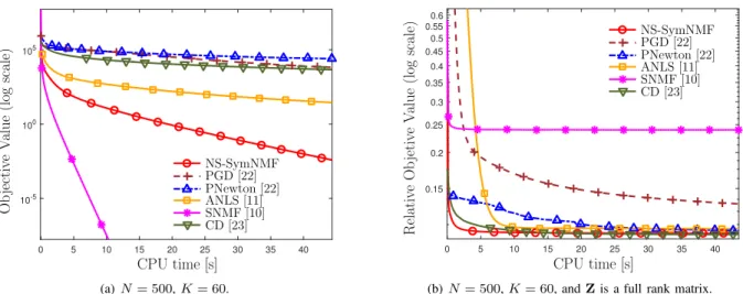
NS-SymNMF PGD [22] PNewton [22] ANLS [11] SNMF [10] CD [23] (a)N= 500,K= 60. Relativ e Ob jetiv e V alue (log scale)
(b)N= 500,K= 60, andZis a full rank matrix. Fig. 1. Data Set I: the convergence behaviors of different SymNMF solvers; each point in the figures is an average of 20 independent MC trials.
Relativ e Ob jetiv e V alue (log scale)
(a) Objective Value
NS-SymNMF PGD [22] PNewton [22] ANLS [11] SNMF [10] CD [23] (b) Optimality Gap
Fig. 2. Data Set II: the convergence behaviors of different SymNMF solvers; each point in the figures is an average of 20 independent MC trials;N= 2000,
K= 4
condition given in [23] for checking whether the generated sequence converges to a unique limit point. A heuristic method for checking the condition is additionally provided, which requires, e.g., plotting the norm between the different iterates.
e) The Proposed NS-SymNMF: The update rule of
NS-SymNMF is similar to that of ANLS. The difference between them is that NS-SymNMF uses one additional block for dual variables and ANLS adds a penalty term. The dual update involved in NS-SymNMF benefits the convergence of the algorithm to KKT points of SymNMF.
We remark that in the implementation of NS-SymNMF we let τ = maxkθk (cf. (7)) and the maximum number of
iterations of GP be40. Also, we gradually increase the value of
ρfrom an initial value to meet condition (12) for accelerating the convergence rate [46]. Here, the choice of ρ follows
ρ(t+1) = min{ρ(t)/(1−ǫ/ρ(t)),6.1N τ} where ǫ= 10−3 as
suggested in [47]. We chooseρ(1)= ¯τfor the case thatZcan
be exactly decomposed and√Nτ¯for the rest of cases, where
¯
τis the mean ofθk,∀k. The similar strategy is also applied for
updatingβ(t). We chooseβ(t)= 6ξ(t)kX(t)Y(t)−Zk2 F/ρ(t)
whereξ(t+1)= min{ξ(t)/(1−ǫ/ξ(t)),1}andξ(1) = 0.01, and
only updateβ(t) once every 100 iterations to save CPU time.
To update Y, we implement the block pivoting method [17] since such method is faster than the GP method for solving the nonnegative least squares problem. If kY(t+1)i k2
2 ≤ τ
is not satisfied, then we switch to GP on Y(t)i . We also remark that we set the step size of PGD to10−5for all tested
cases, and use the Matlab codes of PNewton and ANLS from http://math.ucla.edu/∼dakuang/.
Performance on Synthetic Data. First we describe the two synthetic data sets that we have used in the first part of the numerical results.
Data set I (Random symmetric matrices): We randomly generate two types of symmetric matrices, one is of low rank and the other is of full rank.
For the low rank matrix, we first generate a matrixMwith dimension N ×K, whose entries follow an i.i.d. Gaussian distribution with zero mean and unit variance. We use Mi,j
to denote the(i, j)th entry ofM. Then generate a new matrix
f
Mwhose(i, j)th entry is|Mi,j|. Finally, we obtain a positive
symmetricZ=MfMfT as the given matrix to be decomposed.
For the full rank matrix, we first randomly generate aN×N
in the interval[0,1]. Then we computeZ= (P+PT)/2.
Data set II (Adjacency matrices): One important application of SymNMF is graph partitioning, where the adjacency matrix of a graph is factorized. We randomly generate a graph as follows. First, set the number of nodes to N and the number of cluster to4, and the numbers of nodes within each cluster to 300,500,800,400. Second, we randomly generate data points whose relative distance will be used to construct the adjacency matrix. Specifically, data points {xi} ∈ R, i = 1, . . . , N, are generated in one dimension. Within one cluster, data points follow an i.i.d.Gaussian distribution. The means of the random variables in these 4 clusters are2,3,6,8, respectively, and the variance is 0.5 for all distributions. Construct the similarity matrix A ∈ RN×N, whose (i, j)th
entry is Ai,j= exp(−(xi−xj)2/(2σ2))whereσ2= 0.5.
The convergence behaviors of different SymNMF solvers for the synthetic data sets are shown in Figure 1 and Figure 2. The results are averaged over 20 Monte Carlo (MC) trials with independently generated data. In Figure 1(a), the generatedZ
can be exactly decomposed by SymNMF. It can be observed that NS-SymNMF and SNMF converge to the global optimal solution quickly, and SNMF is the fastest one among all compared algorithms. However, the case where the matrix can be exactly factorized is not common in most practical applications. Hence, we also consider the case where matrixZ
cannot be factorized exactly by aN×Kmatrix. The results are shown in Figure 1(b) and we use the relative objective value for comparison, i.e.,kXXT
−Zk2
F/kZk2F. We can observe that
NS-SymNMF and CD can achieve a lower objective value than other methods. It is worth noting that there is a gap between SNMF and others, since the assumption of SNMF is not satisfied in this case.
We also implement the algorithms on the adjacency matrices (data set II), where the results are shown in Figure 2. The NS-SymNMF and SNMF algorithms converge very fast, but it can be observed that there is still a gap between SNMF and NS-SymNMF as shown in Figure 2(a). We further show the convergence rates with respective to optimality gap versus CPU time in Figure 2(b). The optimality gap (14) measures the closeness between the generated sequence and the true stationary point. To get rid of the effect of the dimension of
Z, we usekX−proj+[X− ∇X(f(X))]k∞as the optimality
gap. It is interesting to see the “swamp” effect [48], where the objective value generated by the CD algorithm remains almost constant during the time period from around 25s to 75s although actually the corresponding iterates do not converge, and then the objective value starts decreasing again.
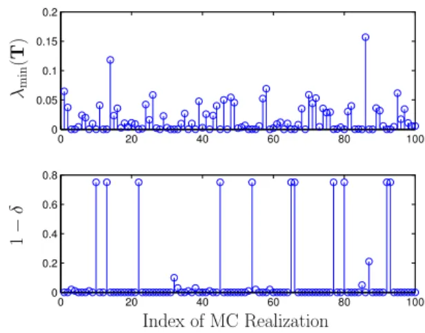
Checking Global/Local Optimality. After the NS-SymNMF algorithm has converged, the local/global optimality can be checked according to Theorem 3 and Theorem 4. To find an appropriateδthat satisfying the condition whereλmin(T)>0,
we initializeδas 1 and decrease it by0.01each time and check the minimum eigenvalue of T. Here, we use data set II with the fixed ratio of the number of nodes within each cluster (i.e., 3 : 5 : 8 : 4) and test on the different total numbers of nodes. The simulation results are shown in Table I with 100 MC trials, where the average value ofλmin(T)andδare
given. Further, the percentage of being able to find a valid
δ >0 that ensures λmin(T)>0 is listed as the last column.
We note that there always existed aδ such thatT is positive definite in all cases that we tested. This indicates that (with high probability) the proposed algorithm converges to a locally optimal solution. In Figure 3, we provide the values ofδthat make the correspondingλmin(T)>0 at each realization.
We also remark that in practice we stop the algorithm in finite steps, so only an approximate KKT point will be obtained, and the degree of such approximation can be measured by the optimality gap defined in (14).
λmin
(
T
)
Fig. 3. Checking local optimality condition, whereN= 500. TABLE I
LOCALOPTIMALITY
N λmin(T) δ Local Optimality (true) 50 2.71×10⁻⁴ 0.42 100% 100 4.16×10⁻⁴ 0.37 100%
500 1.8×10⁻² 0.91 100%
Performance on Real Data.We also implement the algorithm on a few real data sets in clustering applications, which will be described in the next paragraphs.
1) Dense Similarity Matrix: we generate the dense
similarity matrices based on the two real data sets: Reuters-21578 and TDT2 [49]. We use the 10th subset of the processed Reuters-21578 data set, which includes
N = 4,633 documents divided into K = 25 classes. The number of features is 18,933. Topic detection and tracking 2 (TDT2) corpus includes two newswires (APW and NYT), two radio programs (VOA and PRI) and two television programs (CNN and ABC). We use the 10th subset of the processed TDT2 data set withK= 25classes which includes
N = 8,939documents and each of them has 36,771 features. We comment that the 10th TDT2 subset is the largest among the all TDT2 and Reuters subsets. Any other subset can be used equally well. The similarity matrix is constructed by the Gaussian function where the difference between two documents is measured by all features using the Euclidean distance [49].
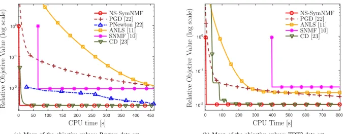
The means and standard deviations of the objective values of the final solutions are shown in Table II. Convergence results of the algorithms are shown in Figure 4. For the Reuters and TDT2 datasets, before SNMF completes the
Relativ e Ob jetiv e V alue (log scale)
(a) Mean of the objective values: Reuters data set
Relativ e Ob jetiv e V alue (log scale)
(b) Mean of the objective values: TDT2 data set
Fig. 4. The convergence behaviors of different SymNMF solvers for the dense similarity matrix; each point in the figures is an average of 20 independent MC trials based on random initializations.
Relativ e Ob jetiv e V alue (log scale)
(a) Mean of the objective values: email-Enron data set
Relativ e Ob jetiv e V alue (log scale)
(b) Mean of the objective values: loc-Brightkite data set
Fig. 5. The convergence behaviors of different SymNMF solvers for the sparse similarity matrix; each point in the figures is an average of 20 independent MC trials based on random initializations.
TABLE II MEAN ANDSTANDARDDEVIATION OFkXXT−Zk2
F/kZk2F OF THEFINALSOLUTION OFEACHALGORITHM BASED ONRANDOMINITIALIZATIONS
Dense Data Sets N K NS-SymNMF PGD [22] PNewton [22] ANLS [11] SNMF [10] CD [23] Reuters [49] 4,633 25 2.65e-3±3.31e-10 1.14e-2±1.18e-5 2.98e-3±3.71e-6 1.16e-2±1.61e-5 9.32e-3 2.66e-3±2.04e-8
TDT2 [49] 8,939 25 1.01e-2±5.35e-9 1.74e-2±7.34e-6 - 2.25e-2±1.25e-6 3.29e-2 1.01e-2±1.21e-6
eigenvalue decomposition for the first iteration, CD and NS-SymNMF have already obtained low objective values. Also, since calculating Hessian in PNewton is time consuming, the result of PNewton is out of range in Figure 4(b).
2) Sparse Similarity Matrix: we also generate multiple
convergence curves for each algorithm with random initializations based on some sparse real data sets.
Email-Enron network data set [50]: Enron email corpus includes around half million emails. We use the relationships between two email addresses to construct the similarity matrix for decomposing. If an address i sent at least one email to addressj, then we take Ai,j=Aj,i= 1. Otherwise,
we set Ai,j=Aj,i= 0.
Brightkite data set [51]: Brightkite was a location-based social networking website. Users were able to share their current
locations by checking-in. The friendships of the users were maintained by Brightkite. The way of constructing the similarity matrix is the same as the Enron email data set.
The means and standard deviations of the objective values of the final solutions are shown in Table III. From the simulation results shown in Figure 5, it can be observed that the NS-SymNMF algorithm converges faster than CD, while SNMF and ANLS converge to some points where the relative objective values are higher than the one obtained by NS-SymNMF.
VI. CONCLUSIONS
In this paper, we propose a nonconvex splitting algorithm for solving the SymNMF problem. We show that the proposed algorithm converges to a KKT point in a sublinear manner.
TABLE III MEAN ANDSTANDARDDEVIATION OFkXXT−Zk2
F/kZk2F OF THEFINALSOLUTION OFEACHALGORITHM BASED ONRANDOMINITIALIZATIONS
Sparse Data Sets N K #nonzero NS-SymNMF ANLS [11] SNMF [10] CD [23] email-Enron [50] 36,692 50 367,662 8.05e-1±4.66e-4 9.18e-1±6.20e-3 9.69e-1 8.13e-1±1.47e-3 loc-Brightkite [51] 58,228 50 428,156 8.75e-1±9.52e-4 9.33e-1±1.93e-3 9.43e-1 8.84e-1±1.49e-3
Further, we provide sufficient conditions to identify global or local optimal solutions of the SymNMF problem. Numerical experiments show that the proposed method can converge quickly to local optimal solutions.
In the future, we plan to extend the proposed methods in a way such that the algorithms can converge to the local or even global optimal solutions of SymNMF without requiring checking conditions. Also, it is possible to apply the nonconvex splitting method to more general matrix factorization problems, such as the quadratic nonnegative matrix factorization problem [52].
VII. APPENDIX
A. Proof of Lemma 1
Sufficiency: the stationary points satisfy
X∗(X∗)T −(ZT +Z)/2X∗,X −X∗ ≥0, ∀X≥0. (30) Let Ω,(X∗(X∗)T −(ZT +Z)/2)X∗/2. We havehΩ,X− X∗i ≥ 0,∀X ≥0. By setting Xappropriately as 0 ≤X≤ X∗, we have Ωi,j ≥ 0,(i, j) ∈ S where S = {i, j|X∗i,j 6= 0}. Also, by setting X appropriately as X ≥ X∗, we have
Ωi,j ≥0,(i, j)∈ S/ . Combining the two cases, we conclude
thatΩ≥0.
From (30), we know thathΩ,Xi ≥ hΩ,X∗i. SinceΩ≥0
and X ≥ 0, we have hΩ,Xi ≥ 0,∀X, meaning that
hΩ,X∗i ≤0. Combining withX∗ ≥0 and Ω≥0, we have
hΩ,X∗i ≥0, which results inhΩ,X∗i= 0. In summary, we have 2 X∗(X∗)T −Z T +Z 2 X∗−Ω= 0, (31a) Ω≥0, (31b) X∗≥0, (31c) hX∗,Ωi= 0, (31d) which are the KKT conditions of the SymNMF problem.
Necessity: If the point is a KKT point of SymNMF, we have
Ω∗= 2 X∗(X∗)T −Z T+Z 2 X∗. (32) Combining with hX∗,Ω∗i= 0, we know that
hΩ∗,X−X∗i ≥0, ∀X≥0, (33) which is the condition of stationary points.
B. Proof of Lemma 2
We prove that ifτis large enough, then the KKT conditions of (1) and (4) are the same.
Proof:It is sufficient to show that whenτis large enough,
there can be no KKT point whose column has sizeτ, leading to the fact that the constraintkX∗kk2≤τ is always inactive.
We check the optimality condition of the SymNMF problem at kX∗kk2 =τk, where τk >0 is a constant. We can rewrite
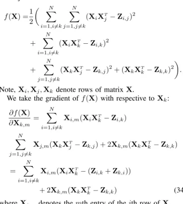
the objective function as
f(X) =1 2 XN i=1,i6=k N X j=1,j6=k (XiXTj −Zi,j)2 + N X i=1,i6=k (XiXTk−Zi,k)2 + N X j=1,j6=k (XkXT j −Zk,j)2+ (XkXTk −Zk,k)2 .
Note,Xi,Xj,Xk denote rows of matrixX.
We take the gradient off(X)with respective toXk: ∂f(X) ∂Xk,m = N X i=1,i6=k Xi,m(XiXTk−Zi,k) N X j=1,j6=k Xj,m(XkXT j −Zk,j) + 2Xk,m(XkXTk−Zk,k) = N X i=1,i6=k
Xi,m(XiXTk−(Zi,k+Zk,i))
+ 2Xk,m(XkXTk−Zk,k) (34)
whereXi,m denotes themth entry of theith row ofX.
Assume thatX∗k is a KKT point. We have(∂f(X∗k) ∂Xk )(Xk− X∗k)T ≥0,∀ X k ∈ X, where X ={Xk|Xk ≥0,kXkk2 ≤ τk}, which implies ∂f(X∗k) ∂Xk,m (Xk,m−X∗k,m)≥0 0≤Xk,m≤X∗k,m= v u u tτk− K X n=1,n6=m (X∗k,n)2 ∀ m. (35)
Since kX∗kk2 = τk, there exists an index m such that
X∗k,m > 0. Consider a feasible point 0 ≤ Xk,m < X∗k,m,
wherem∈ Sm,{m|X∗k,m6= 0}. Thanks to (35), we have ∂f(X∗k,m)
∂Xk,m ≤
0, 0≤Xk,m<X∗k,m ∀m∈ Sm. (36)
Plugging (34) into (36) and multiplyingX∗
k,mon both sides of (36), we can obtain X∗k,m XN i=1,i6=k X∗i,m X∗i(X∗k)T −Zi,k+2 Zk,i +X∗k,m(X∗k(X∗k)T −Zk,k) ≤0 ∀ m∈ Sm. (37)
For the case m /∈ Sm, we know thatX∗k,m= 0. Summing
up (37) ∀m, and noting that|Sm| ≥1we can get
p, N X i=1,i6=k X∗i(X∗k)T X∗ i(X ∗ k) T −Zi,k+2 Zk,i | {z } ,Mi,k +X∗k(X∗k)T (X∗k(X∗k)T −Zk,k)≤0. (38)
In (38), Mi,k is a quadratic function with respective to Ci,k, where Ci,k , X∗i(X∗k)
T
, so the minimum of Mi,k
is −1/4((Zi,k +Zk,i)/2)2. Consequently, the minimum of
PN
i=1,i6=kMi,k is−1/4
PN
i=1,i6=k((Zi,k+Zk,i)/2)2.
In addition, since we havekX∗kk2=τk, the lower bound of pis pL,−1/4PNi=1,i6=k((Zi,k+Zk,i)/2)2+τk(τk−Zk,k)
which is a quadratic function in terms of τk. Therefore, if
τk > θk ,
Zk,k+12qPNi=1(Zi,k+Zk,i)2
2 , (39)
then p≥pL >0, which contradicts the optimality condition
(37). It can be concluded that whenever τk is large enough,
at any KKT point no column will have size equal to τk.
Furthermore, it can be easily checked that τ > maxkθk is
a sufficient condition. The proof is complete.
C. Convergence Proof of the Proposed Algorithm
In this section, we prove Theorem 1. The analysis consists of a series of lemmas.
Lemma 3. Consider using the update rules(8)–(10)to solve
problem (1). Then we have
kΛ(t+1)−Λ(t)k2F ≤3N2τ2kX(t+1)−X(t)k2F
+ 3kX(t)(Y(t))T
−Zk2FkY(t+1)−Y(t)k2F
+ 3N τkX(t)(Y(t+1)−Y(t))T
k2F. (40)
Proof:The optimality condition of theXsubproblem (9)
is given by
(X(t+1)(Y(t+1))T
−Z)Y(t+1)
+ρ(X(t+1)−Y(t+1)+Λ(t)/ρ) = 0. (41) Substituting (10) into (41), we have
Λ(t+1)=−(X(t+1)(Y(t+1))T
−Z)Y(t+1). (42) Subtracting the same equation in iteration t, we have the successive difference of the dual matrix (44), shown at the top of the next page.
Note that the following is true
Q=1 2 X (t)(Y(t+1) −Y(t))T(Y(t+1) −Y(t)) + 2X(t)(Y(t))T(Y(t+1) −Y(t)) +1 2X (t)(Y(t+1) −Y(t))T(Y(t+1)+Y(t)) =X(t)(Y(t))T(Y(t+1) −Y(t)) +X(t)(Y(t+1)−Y(t))TY(t+1). (45)
Plugging (45) into (44), we have
Λ(t+1)−Λ(t) =Z(Y(t+1)−Y(t))−(X(t+1)−X(t))(Y(t+1))TY(t+1) −X(t)(Y(t))T(Y(t+1) −Y(t)) −X(t)(Y(t+1)−Y(t))Y(t+1) =(Z−X(t)(Y(t))T)(Y(t+1) −Y(t)) −(X(t+1)−X(t))(Y(t+1))T Y(t+1) −X(t)(Y(t+1)−Y(t))TY(t+1). (46)
Using triangle inequality, we arrive at
kΛ(t+1)−Λ(t)kF ≤ kX(t+1)−X(t)kFk(Y(t+1))TY(t+1)kF +kX(t)(Y(t))T
−ZkFkY(t+1)−Y(t)kF +kX(t)(Y(t+1)−Y(t))T
kFkY(t+1)kF. (47)
Since kYik2 ≤ τ, we know that kYkF ≤
√
N τ. Squaring both sides of (47), we obtain
kΛ(t+1)−Λ(t)k2F ≤3N2τ2kX(t+1)−X(t)k2F
+ 3kX(t)(Y(t))T
−Zk2FkY(t+1)−Y(t)k2F
+ 3N τkX(t)(Y(t+1)−Y(t))T
k2F. (48)
The claim is proved.
In the second step, we bound the successive difference of the augmented Lagrangian.
Lemma 4. Consider using the update rules(8)–(10). If
ρ >6N τ and β(t)> 6 ρkX (t)(Y(t))T −Zk2F−ρ, (49) we have L(X(t+1),Y(t+1),Λ(t+1))− L(X(t),Y(t),Λ(t)) ≤ −c1kX(t+1)−X(t)k2F−c2kX(t)(Y(t+1)−Y(t))Tk2F −c3kY(t+1)−Y(t)k2F (50)
wherec1, c2, c3>0 are some positive constants.
Proof:Let b L(X(t),Y,Λ(t)), 1 2kX (t)YT −Zk2F +ρ 2kX (t) −Y+Λ(t)/ρk2F+ β(t) 2 kY−Y (t) k2F, (51)
which is an upper bound ofL(X(t),Y,Λ(t)), and
A,L(X(t),Y(t+1),Λ(t))− L(X(t),Y(t),Λ(t)),
B,L(X(t+1),Y(t+1),Λ(t))− L(X(t),Y(t+1),Λ(t)),
C,L(X(t+1),Y(t+1),Λ(t+1))− L(X(t+1),Y(t+1),Λ(t)),
b
A,Lb(X(t),Y(t+1),Λ(t))− L(X(t),Y(t),Λ(t)).
We have the following descent estimate
L(X(t+1),Y(t+1),Λ(t+1))− L(X(t),Y(t),Λ(t))
Λ(t+1)−Λ(t)=−hX(t+1)(Y(t+1))TY(t+1) −X(t)(Y(t))TY(t) −Z(Y(t+1)−Y(t))i (43) =−h(X(t+1)−X(t))(Y(t+1))TY(t+1)+X(t) (Y(t+1))TY(t+1) −(Y(t))TY(t)+Z(Y(t+1) −Y(t))i =Z(Y(t+1)−Y(t))−(X(t+1)−X(t))(Y(t+1))TY(t+1) −1 2 X (t) (Y(t+1)+Y(t))T(Y(t+1)−Y(t)) + (Y(t+1)−Y(t))T(Y(t+1)+Y(t)) | {z } ,Q . (44)
Next we bound the quantities in (52)
b A=1 2kX (t)(Y(t+1))T −Zk2F−1 2kX (t)(Y(t))T −Zk2F +ρ 2kX (t) −Y(t+1)+Λ(t)/ρk2F −ρ2kX(t)−Y(t)+Λ(t)/ρk2F+ β(t) 2 kY (t+1) −Y(t)k2F (a) =h(X(t)(Y(t+1))T −Z)X(t),Y(t+1)−Y(t)i −1 2kX (t)(Y(t+1)−Y(t))T k2 F +ρhX(t)−Y(t+1)+Λ(t)/ρ,Y(t+1)−Y(t)i −ρ2kY(t+1)−Y(t)k2F+β (t) 2 kY (t+1) −Y(t)k2F (b) ≤ − 12kX(t)(Y(t+1)−Y(t))T k2F− ρ 2kY (t+1) −Y(t)k2F −β (t) 2 kY (t+1) −Y(t)k2F
where(a)is due to the fact that Taylor expansion for quadratic problems is exact, and (b)is due to the optimality condition for problem (8). Similarly, we have
B ≤ −12k(X(t+1)−X(t))(Y(t+1))T k2F −ρ 2kX (t+1) −X(t)k2F, (53) C=hX(t+1)−Y(t+1),Λ(t+1)−Λ(t)i (a) =1 ρkΛ (t+1) −Λ(t)k2F (54) where(a)is from (10).
Substituting the result of Lemma 3 into (54), we can obtain
L(X(t+1),Y(t+1),Λ(t+1))− L(X(t),Y(t),Λ(t)) ≤ − ρ 2 − 3N2τ2 ρ kX(t+1)−X(t)k2F − 1 2− 3N τ ρ kX(t)(Y(t+1)−Y(t))T k2F − ρ 2+ β(t) 2 − 3kX(t)(Y(t))T −Zk2 F ρ kY(t+1)−Y(t)k2F −12k(X(t+1)−X(t))(Y(t+1))T k2F. (55) Therefore, from (55) if ρ2−3N2τ2 ρ >0, 1 2− 3N τ ρ >0, and ρ+β(t) 2 − 3kX(t)(Y(t))T−Zk2 F ρ >0, (56)
which are equivalent to
ρ >6N τ and β(t)>6kX (t)(Y(t))T −Zk2 F−ρ2 ρ , (57) thenL(X(t+1),Y(t+1),Λ(t+1))− L(X(t),Y(t),Λ(t))<0. Then, it is concluded that L(X(t+1),Y(t+1),Λ(t+1)) is decreasing.
In the next step we prove thatL(X(t+1),Y(t+1),Λ(t+1))is lower bounded.
Lemma 5. Consider using the update rules (8) (9) (10). If
ρ≥N τ is satisfied, we have
L(X(t+1),Y(t+1),Λ(t+1))≥0. (58)
Proof:At iterationt+ 1, the augmented Lagrangian can
be lower bounded as L(X(t+1),Y(t+1),Λ(t+1)) =1 2kX (t+1)(Y(t+1))T −Zk2F+hX(t+1)−Y(t+1),Λ(t+1)i +ρ 2kX (t+1)−Y(t+1)k2 F (a) =1 2kX (t+1)(Y(t+1))T −Zk2F +hX(t+1)−Y(t+1),−(X(t+1)(Y(t+1))T −Z)Y(t+1)i +ρ 2kX (t+1) −Y(t+1)k2F (b) ≥12(ρ−N τ)kX(t+1)−Y(t+1)k2F (59) where(a)is due to (42), and (b)is true because
0≤k(X(t+1)−Y(t+1))(Y(t+1))T −(X(t+1)(Y(t+1))T −Z)k2F =k(X(t+1)−Y(t+1))(Y(t+1))T k2F −2h(Y(t+1))T(X(t+1) −Y(t+1)),X(t+1)(Y(t+1))T −Zi +kX(t+1)(Y(t+1))T −Z)k2F, andkYk2F ≤N τ.
From (59), we know that if ρ ≥ N τ, we have
L(X(t+1),Y(t+1),Λ(t+1))≥0.
These lemmas lead to the main convergence claim.
Proof:Combing (50) and (58), we have
lim t→∞kX (t+1) −X(t)k2F = 0, (60) lim t→∞kX (t)(Y(t+1) −Y(t))T k2F = 0, lim t→∞kX (t)(Y(t))T −Zk2FkY(t+1)−Y(t)k2F = 0.
By Lemma 3, we have
lim t→∞kΛ
(t+1)
−Λ(t)k2F = 0, (61) which implieslimt→∞kX(t)−Y(t)k2F = 0. Combining with
(60), we can further know thatlimt→∞kY(t+1)−Y(t)k2F = 0.
The boundedness assumption of X(t) then follows from the
boundedness of Y(t). Using the expression of Λ(t) in (42),
one can show that{Λ(t)} is also bounded. The optimality condition of (8) is given by
(X(t))T(X(t)(Y(t+1))T −Z)−ρ(X(t)−Y(t+1)+Λ(t)/ρ)T +β(t)(Y(t+1)−Y(t))T,(Y −Y(t+1))T ≥0, ∀Y≥0 and kYik22≤τ ∀i. (62)
Substituting (42) into (62), using (60), and taking limit over any converging subsequence of {X(t),Y(t),Λ(t)}, we have
h(X∗)T(X∗(Y∗)T −Z) + ((X∗(Y∗)T −Z)Y∗)T −ρ(X∗−Y∗)T ,(Y−Y∗)T i ≥0, ∀Y≥0 and kYik22≤τ∀i. (63)
The optimality condition of (9) is given by
(X(t+1)(Y(t+1))T
−Z)(Y(t+1))
+ρ(X(t+1)−Y(t+1)+Λ(t)/ρ) = 0. (64) Taking limit of (64) over the same subsequence, we have
(X∗(Y∗)T
−Z)Y∗+ρ(X∗−Y∗+Λ∗/ρ) = 0. (65) Using the factX∗=Y∗, we have
X∗(X∗)T −Z T +Z 2 X∗,X−X∗ ≥0, ∀X≥0, kXik22≤τ∀i, (66) (X∗(X∗)T −Z)X∗+Λ∗= 0, (67)
which are the KKT conditions of problem (1).
D. Convergence Rate Proof of the Proposed Algorithm
Proof: Based on Theorem 1,kX(t)k2F is bounded. There
must exist a finiteγ >0such that kX(t)k2
F ≤N γ,∀t, where γ is only dependent onτ,N andkZkF.
From the optimality condition of Yin (8), we have
(Y(t+1))T = projY (Y(t+1))T −((X(t))T(X(t)(Y(t+1))T −Z)−ρ(X(t) −Y(t+1)+Λ(t)/ρ)T +β(t)(Y(t+1)−Y(t))T) . Then, we have (Y(t))T−projY (Y(t))T −((X(t))T(X(t)(Y(t))T −Z) −ρ(X(t)−Y(t)+Λ(t)/ρ)T) F = (Y(t))T −(Y(t+1))T+ (Y(t+1))T −projY(Y(t))T −((X(t))T(X(t)(Y(t))T −Z) −ρ(X(t)−Y(t)+Λ(t)/ρ)T ) F (a) ≤ kY(t)−Y(t+1)kF + projY (Y(t+1))T −((X(t))T (X(t)(Y(t+1))T −Z) −ρ(X(t)−Y(t+1)+Λ(t)/ρ)T +β(t)(Y(t+1)−Y(t))T) −projY(Y(t))T −((X(t))T(X(t)(Y(t))T −Z) −ρ(X(t)−Y(t)+Λ(t)/ρ)T ) F (b) ≤(2 +ρ+β(t))kY(t+1)−Y(t)kF +k(X(t))TX(t)(Y(t+1) −Y(t))T kF (c) ≤(2 +ρ+β(t))kY(t+1)−Y(t)kF +pN γkX(t)(Y(t+1)−Y(t))T kF (68)
where projY denotes the projection of Y to the feasible space; in (a) we used triangle inequality; (b) is due to the nonexpansiveness of the projection operator; and(c)is due to the boundedness ofkXkF.
Similarly, we can bound the size of the gradient of the augmented Lagrangian with respect to X by the following series of inequalities k∇XL(X(t),Y(t),Λ(t))kF =k(X(t)(Y(t))T −Z)Y(t) +ρ(X(t)−Y(t)+Λ(t)/ρ)kF (a) =(X(t)(Y(t))T −Z)Y(t)+ρ(X(t)−Y(t)+Λ(t)/ρ) −((X(t+1)(Y(t+1))T −Z)Y(t+1) +ρ(X(t+1)−Y(t+1)+Λ(t)/ρ))F ≤ k(X(t)(Y(t))T −Z)Y(t) −((X(t+1)(Y(t+1))T −Z)Y(t+1))kF +ρkY(t+1)−Y(t)kF+ρkX(t+1)−X(t)kF (69) (b) =kΛ(t+1)−Λ(t)kF+ρkY(t+1)−Y(t)kF +ρkX(t+1)−X(t)kF (70)
where (a) is from the optimality condition of the
X-subproblem (41); (b) is true due to (43) and (42). Squaring both sides of (70) and applying Lemma 3, we have
k∇XL(X(t),Y(t),Λ(t))k2F ≤3(3N2τ2+ρ2)kX(t+1)−X(t)k2 F + 3(3kX(t)(Y(t))T −Zk2F+ρ2)kY(t+1)−Y(t)k2 F + 9N τkX(t)(Y(t+1)−Y(t))T k2F. (71)
Due to the boundedness of X(t) andY(t), we must have that for some δ >0,kX(t)(Y(t))T−Zk
F ≤δ.
Therefore, combining (68) and (71), there must exists a finite positive numberσ1 such that
k∇Le (X(t),Y(t),Λ(t))k2 F ≤σ1F (72) where F ,kX(t+1)−X(t)kF2 +kY(t+1)−Y(t)k2F +kX(t)(Y(t+1)−Y(t))T k2F (73)
In particular, we have σ1 ,max{3(3N2τ2+ρ2),3(2 +ρ+ β(t))2+ 3(3δ2+ρ2),3γ+ 9N τ} andβ(t)≤6δ2/ρ.
According to Lemma 3, we have
kX(t+1)−Y(t+1)k2F= 1 ρ2kΛ
(t+1)−Λ(t)k2
F ≤σ2F (74)
where some constantσ2,max{3N2τ2/ρ2,3δ2/ρ2,3N τ /ρ2}.
Also, we have kX(t)−Y(t)kF =kX(t)−X(t+1)+X(t+1)−Y(t+1)+Y(t+1)−Y(t)kF ≤kX(t)−X(t+1)kF +kX(t+1)−Y(t+1)kF +kY(t+1)−Y(t)kF, (75) which yields kX(t)−Y(t)k2F ≤σ3F (76) forσ3,max{9N2τ2/ρ2+ 3,9δ2/ρ2+ 3,9N τ /ρ2}.
The inequalities (72) and (76) imply that
k∇Le (X(t),Y(t),Λ(t))k2F +kX(t)−Y(t)k2F ≤(σ1+σ3)F.
(77) According to Lemma 4, there exists a constant σ4 , min{c1, c2, c3}such that
L(X(t),Y(t),Λ(t))− L(X(t+1),Y(t+1),Λ(t+1))≥σ4F.
(78) Combining (77) and (78), we have
k∇Le (X(t),Y(t),Λ(t)k2F+kX(t)−Y(t)k2F ≤
σ1+σ3 σ4
(L(X(t),Y(t),Λ(t))−L(X(t+1),Y(t+1),Λ(t+1))).
(79) Summing both sides of (79) over t= 1, . . . , r, we have
r X t=1 k∇Le (X(t),Y(t),Λ(t))k2F+kX(t)−Y(t)k2F ≤σ1σ+σ3 4 (L(X(1),Y(1),Λ(1))− L(X(t+1),Y(t+1),Λ(t+1))) (a) ≤σ1σ+σ3 4 L (X(1),Y(1),Λ(1)) (80) where(a)is due to Lemma 5.
According to the definition ofT(ǫ)andP(X(t),Y(t),Λ(t)), the above inequality becomes
T(ǫ)ǫ≤ σ1+σ3
σ4 L
(X(1),Y(1),Λ(1)). (81) Dividing both sides by T(ǫ), and by setting C , (σ1+ σ3)/σ4, the desired result is obtained.
E. Sufficient Condition of Global Optimality
Proof: Let Ω be the Lagrange multipliers matrix. The
Lagrangian of problem (1) is given by
L(X,Ω) =1
2Tr((XX
T
−Z)T(XXT
−Z))− hX,Ωi. (82)
Let (X∗,Ω∗) be a KKT point of problem (1). To show global optimality of (X∗,Ω∗), it is sufficient to prove the
following saddle point condition [42, pp. 238]
L(X∗,Ω)≤ L(X∗,Ω∗)≤ L(X,Ω∗), ∀ Ω≥0, ∀ X. (83) To show the left hand side of (83), we have the following
L(X∗,Ω∗)− L(X∗,Ω) =−hX∗,Ω∗i −(−hX∗,Ωi) =hX∗,Ω−Ω∗i(a)=hX∗,Ωi
(b)
≥0. (84)
where(a)is due to (5d), and (b)is due toΩ≥0 and (5c). Next we show the right hand side of (83)
L(X,Ω∗)− L(X∗,Ω∗) =1 2Tr[(XX T −X∗(X∗)T)(XXT −X∗(X∗)T)] | {z } ,M +Tr[(X∗(X∗)T −ZT)(XXT −X∗(X∗)T)] − hX−X∗,Ω∗i (a) ≥ hX−X∗, X∗(X∗)T −Z T+Z 2 (X+X∗)i (85) − hX−X∗,Ω∗i (b) =hX−X∗, X∗(X∗)T −Z T+Z 2 (X−X∗)i =Tr(X−X∗)T X∗(X∗)T −Z T+Z 2 | {z } ,S (X−X∗) (86)
where(a)is due toM ≥0 and the fact that
XXT −X∗(X∗)T = 1 2 (X+X∗)(X−X∗)T +(X−X∗)(X+X∗)T; (87)
(b) is true because of (5a). Clearly, if we have S 0, then the following inequality must be true
L(X,Ω∗)− L(X∗,Ω∗)≥0.
F. Sufficient Condition of Local Optimality
Proof: We first simplify the termMin (85) as follows.
1 2Tr[(XX T −X∗(X∗)T)T(XXT −X∗(X∗)T)] (a) =1 2Tr ((X−X∗)XT+X∗(X−X∗)T)T ((X−X∗)XT +X∗(X −X∗)T) (b) =1 2Tr Yb(Yb +X ∗)T+X∗YbTT b Y(Yb +X∗)T +X∗YbT (c) =1 2Tr UTU+X∗YbTU+Yb(X∗)TU+X∗YbTU +X∗YbTYb(X∗)T +X∗YbTX∗YbT +Yb(X∗)TU+Yb(X∗)TYb(X∗)T +Yb(X∗)TX∗YbT =1 2Tr h UUT+ 4UX∗YbT + 2Yb(X∗)TX∗YbTi +TrhX∗YbTX∗YbTi =1 2Tr b Yh YbT I i I 4X∗ 0 2(X∗)TX∗ h b YT I iT b YT +TrhX∗YbTX∗YbTi (88) where(a)is due to the fact that
XXT
−X∗(X∗)T = (X
−X∗)XT +X∗(X
−X∗)T;
(89) in (b) we defined Yb ,X−X∗ which shows the difference betweenXandX∗; and in(c)we definedU,YbYbT =UT.
Combining (86) and (88), we have
L(X,Ω∗)− L(X∗,Ω∗) =Tr b Y 1 2Yb TYb + 2YbTX∗+ (X∗)TX∗ b YT +Tr h X∗YbTX∗YbTi+ Tr b YT X∗(X∗)T −Z T +Z 2 b Y = K X m K X n (Yb′m)T Km,nYb′n+ K X m K X n (Yb′m)Te Km,nYb′n + K X m (Yb′m)TSYb′ m =vec(Yb)TT vec(Yb) where T, K1,1I+Ke1,1+S · · · K1,KI+Ke1,K .. . · · · ... KK,1I+KeK,1 · · · KK,KI+KeK,K+S , Km,n, 1 2(Yb ′ m)TYb′n+ 2(Ybm′ )TX′∗n + (X′∗m)TX′∗n, (90)
and Kem,n ,X′∗n(Xm′∗)T, (m, n) denotes the (m, n)th block
of a matrix, X′∗m (Yb′n) denotes the mth (or nth) column of matrix X∗ (orYb).
For the(m, n)th block, we have
(Yb′m)T 1 2(Yb ′ m) TYb′ n+ 2(Yb′m) TX′∗ n + (X′∗m) TX′∗ n I +X′∗n(X′∗m)T+δ m,nS b Yn′ (a) ≥(Yb′m)T −14kYbm′ k22+kYb′nk22−1 δkYb ′ mk22 −δkX′∗nk22+ (X′∗m)TX′∗ n I+X′∗n(X′∗m)T +δ m,nS b Yn′ =(Yb′m)T −(1 4 + 1 δ)kYb ′ mk22− 1 4kYb ′ nk22 b Y′n + (Yb′m)T (X′∗m)TX′∗ n −δkX′∗nk22 I+X′∗n(X′∗m)T +δm,nS b Y′n (b) ≥kYbm′ kkYb′nk −(1 4 + 1 δ)kYb ′ mk22− 1 4kYb ′ nk22 + (Yb′m)TT m,nYb′n where Tm,n, (X′∗m) TX′∗ n −δkX′∗nk22 I+X′∗n(X′∗m)T+δ m,nS, δm,nis the Kronecker delta function, andTm,nis the(m, n)th
block of matrix T, and (a) we use triangle inequality and
δ > 0 is any positive number; (b) we use Cauchy-Schwarz inequality.
If there exists δ such that T is positive definite, then X∗
is a strict local minimum point of problem (1). That is, there exist someγ, ǫ >0 such that
L(X,Ω∗)− L(X∗,Ω∗)≥γ2kX−X∗k2F, ∀ Xsuch thatkX′m−X′∗mk22≤ǫ, (91) whereγis given by γ=− 2K2 δ +K(K−2) ǫ2+ 2λmin(T) (92)
whereλmin(T)is the smallest eigenvalue of matrixT. Clearly γ can be made positive for sufficiently smallǫ.
According to the definition of Lagrangian (82), we have
L(X,Ω∗) =f(X)− hX,Ω∗i. (93) Combing with (91) and KKT conditions (5b)–(5d), we can obtain f(X)≥ L(X,Ω∗)≥f(X∗) +γ 2kX−X ∗ k22, ∀ X≥0such that kX−X∗k ≤ǫ. (94) ThereforeX∗ is a strict local minimum point of problem (1).
G. Sufficient Local Optimality Condition WhenK= 1
Proof:The termM is as follows.
M=1 2Tr[Yb[ Yb T I ] I 4X∗ 0 2(X∗)TX∗ [ YbT I ]TYbT] +Tr h X∗YbTX∗YbTi. (95)