Invariants of binary forms

(1)

Invariants of binary forms

Inauguraldissertation

zur

Erlangung der Würde eines Doktors der Philosophie

vorgelegt der

Philosophisch-Naturwissenschaftlichen Fakultät

der Universität Basel

von

Mihaela Ileana Popoviciu Draisma

von Rumänien

(2)

auf Antrag von

Prof. Dr. Hanspeter Kraft und Prof. Dr. Jerzy Weyman

Basel, den 12. November 2013

(3)

Acknowledgments

I thank Hanspeter Kraft for trusting me with the study of invariants, for oering

me this work that gave me joy and inspiration, for his guidance and advice.

I thank Andries Brouwer for being such a nice and supportive collaborator and

co-author. It is a joy and an honour to work with him.

I thank Jerzy Weyman for the crash course on invariant theory he gave me in

the short moments we met in Basel and Boston.

I thank Varga Csaba, one of the brightest gures from my childhood and later

times. His maths circles were spots of light in the gray of communistic

school-time.

I thank my professors at Babes-Bolyai University and at Kaiserslautern

Univer-sity for the many inspiring lectures. I thank my colleagues and friends at the

Mathematical Institute Basel for the nice moments we had together.

I thank Renate and Hanspeter for hosting me in Basel whenever I came there

for working on my thesis, for listening to me, encouraging me, and supporting

me in their kind way. I thank them and my friends Joswitte, Simon, Regula,

Andreas, Jonas, Monika, Marine, Stéphane, Sebastian, Christoph, and Jaqueline

for making returning to Basel feel like returning to a second home.

I thank Oana, Catalin, and Marius for being such good friends, despite the

geographical distance. I thank my friends and relatives in the Netherlands for

their support.

I thank my parents, especially my mother, for unconditionally coming to help

me whenever I need.

I thank Jan and Mirona for making my days so bright.

(4)

Introduction

We work over the eld

C

of complex numbers. We denote by

SL

2

the group

of complex 2

×

2-matrices with determinant 1. Let

Vn

=

C

[

x, y

]

n

be the

SL

2

-module of binary forms (homogeneous polynomials in

x

and

y

of degree

n

), on

which

SL

2

acts via

g

· f

(

v

) =

f

(

g

−1

v

)

,

for

g

∈

SL

2

,

f

∈

C

[

x, y

]

and

v

∈

C

2

. The algebra of polynomial functions on

Vn

, denoted by

O(

Vn

)

, is a polynomial ring in

n

+ 1

variables. The group

SL

2

acts on

O(

Vn

)

via the action

g

· j

(

f

) =

j

(

g

−1

· f

)

,

for

g

∈

SL

2

,

j

∈ O(

V

n

)

and

f

∈

V

n

. An invariant of

V

n

is an element

j

∈ O(

V

n

)

such that

g

· j

=

j

for all

g

∈

SL

2

. The set of invariants of

V

n

forms the algebra

of invariants

I

:=

O(

V

n

)

SL2

.

The theory of invariants originated in England about the middle

of the nineteenth century as the genuine analytic instrument for

describing congurations and their inner geometric relations in

pro-jective geometry. The functions and algebraic relations expressing

them in terms of projective coordinates are to be invariant under all

homogeneous linear transformations. ([Wey46, page 27])

In the nineteenth century mathematicians studied invariants of binary forms

motivated by the philosophy that `any' property of polynomials unaected by

linear transformations can be expressed by the vanishing of invariants. The

polynomial

ax

2

_{+ 2}

_bx

₊

_c

_{for example has a double root if and only if the}

invariant

b

2

₋

_ac

_of

_ax

2

_{+ 2}

_bxy

₊

_cy

2

_{vanishes. Consider, as another example,}

the non-zero quartic

q

(

x, y

) =

ax

4

₊

_bx

3

_y

₊

_{. . .}

₊

_ey

4

_{; the solutions of the equation}

q

(

x, y

) = 0

correspond to 4 points on the projective line. These four points form

a harmonic division if and only if the invariant

j

3

=

a

b

c

b

c

d

c

d

e

7

(8)

of the quartic

q

vanishes (cf. Dixmier [Dix90], p.42). The invariants of binary

forms are related to the study of algebraic equations as well. For example,

the binary form

q

(

x, y

)

of degree 5 has an invariant of degree 18 with a nice

property: if this invariant vanishes, then the equation

q

(

x,

1) = 0

can be solved

by radicals (cf. Dixmier [Dix90], p.43).

Early in the 1800s it was known that the invariants of

V

2

are spanned by

the discriminant

b

2

₋

_ac

_of

_ax

2

_{+ 2}

_bxy

₊

_cy

2

_{, and that the invariants of}

_V

3

are

generated by the discriminant

(

ad

−

bc

)

2

₋

₄₍

_ac

₋

_b

2

₎₍

_bd

₋

_c

2

₎

_of

_ax

3

_{+ 3}

_bx

2

_y

₊

3 cxy

2

₊

_dy

3

_{. About the binary forms}

_ax

4

_{+ 4}

_bx

3

_y

₊

_{. . .}

₊

_ey

4

_{of degree 4 it}

was known that the invariant

j

3

dened above and

j

2

=

ae

−

4 bd

+ 3

c

2

are

algebraically independent and generate the invariants of

V

4

. The invariants

j

2

and

j

3

were discovered in the period 1840-1850 by Boole, Cayley, Eisenstein

(cf. Dixmier [Dix90], p.41). Regarding the invariants of

V

5

, Hermite ([Her54])

proved in 1854 that they were generated by 4 irreducible invariants of degrees

4, 8, 12, and 18. Before that, only the invariants of degrees 4, 8, and 12 had

been known, and for a long time people believed that all invariants of

V

5

had

degrees divisible by 4 (cf. Dixmier [Dix90], p.41).

Cayley [Cay56] claimed in 1856 that that the algebra

I

of invariants of

V

n

had no nite bases for the cases

n

= 7

and

n

= 8

. However, twelve years later,

in 1868, Gordan [Gor68] proved the contrary: he showed that

I

has a nite basis

for all

n

.

Im

146

sten

_{Bande der Philosophical Transactions pag. 101 hat Herr}

Cayley sich mit der Frage beschäftigt, ob alle aus einer binären

Form entstehenden Covarianten und Invarianten als ganze

Functio-nen einer begrenzten Anzahl von Former mit numerischen

Coe-cienten darstellbar seien; er hat gezeigt, dass bei Formen zweiten,

dritten und vierten Grades sich alles in der verlangten Weise

aus-drücken lässt. Im Folgenden gebe ich für binäre Formen

n

ten

Grades

ein endliches System von Covarianten und Invarianten an, von

de-nen ich zeige, dass und wie alle aus der Form abgeleitete Formen

sich als ganze rationale Functionen derselben mit numerischen

Coef-cienten darstellen lassen. Dieses für den allgemeinen Fall gegebene

System ist immer zu gross und lässt sich in jedem besonderen Falle

reduciren; für Formen fünften und sechsten Grades habe ich auch

diese Reduction ausgeführt und ein möglichst kleines System von

Grundformen geliefert. ([Gor68])

The study of invariants of binary forms was an important part of a new

disci-pline, die neue Algebra (the new Algebra), as Clebsch named it in 1872. At

that time Clebsch wrote that

die fundamentalen Untersuchungen von Gordan über die Endlichkeit

der Formensysteme [

. . .

] eine Perspective in eine neue Classe tiefer

und wichtiger Forschungen errönet.[Cle72]

About twenty years later, in 1890, Hilbert [Hil90] generalised the result of

Gor-dan to a system of several homogeneous forms in a nite number of variables.

(9)

His proof was non-constructive and did not provide any tools to determine such

nite bases. Hilbert `only' proved that these nite bases existed, to which

Gor-dan reacted with the famous exclamation ([Rei96]):

Das ist nicht Mathematik. Das ist Theologie.

Hilbert [Hil93] returned to the problem and in 1893 gave a proof which was

this time constructive. Eventually Gordan appreciated Hilbert's new ideas,

remarking

I have convinced myself that Theology also has its merits.[Rei96]

With his article from 1893 Hilbert opened a new chapter in mathematics: the

article contains famous results such as Hilbert's basis theorem and Hilbert's

Nullstellensatz (as they are known nowadays), without which it is hard to

imagine the mathematics of today.

It is known, hence, since the nineteenth century, that the algebra

I

of

in-variants of binary forms of degree

n

is nitely generated over

_C

, i.e. there exist

nitely many invariants

j

1

, . . . , j

r

∈

I

, such that

I

=

C

[

j

1

, . . . , j

r

]

. Nevertheless,

nding the generators of

I

is, in general, a dicult problem. Two methods were

developed in the nineteenth century: the symbolic method, and the enumerative

method.

The symbolic method was developed by Aronhold and Clebsch in the middle

of the nineteenth century. Called by Hermann Weyl the great war-horse of

nineteenth century invariant theory, the symbolic calculus allows the reduction

of the computations with binary forms of degree

n

to the special cases of the

n

th

power of a linear form

(

α

1

x

+

α

2

y

)

n

. The classics proved that the invariants

of binary forms have symbolic representations as products of factors of type

[

αβ

]

, where

[

αβ

]

stands for the determinant

α

1

β

2

−

α

2

β

1

. The manipulation of

invariants got simplied by representing them in succinct symbolic expressions.

Kung & Rota [KR84] gave in 1984 a rigorous and yet manageable account of the

umbral or symbolic calculus that was performed in the nineteenth century (see

also Chap.

2.2). With the help of the symbolic method, Gordan [Gor68] proved,

in 1868, that the covariants of a binary form

f

of degree

n

are generated by a

nite number of iterated transvectants

f,

(

f, f

)

d

,

(

f,

(

f, f

)

d

)

e

, . . .

. For a modern

interpretation of Gordan's algorithm we refer to Weyman [Wey93]. Gordan's

proof was constructive and provided sets of generators for the invariants and

covariants of

V

6

([Gor87]). Following Gordan's method, von Gall [Gal88] found

in 1888 a set of generating covariants of

V

7

, but this set was not minimal. In

two papers published in 1880, von Gall [Gal80] computed a set of generating

covariants of

V

8

, but this set was again not minimal (he did found the correct

number of the generating invariants of

V

8

). No sets of generating invariants

of covariants of

Vn

for

n

≥

9 were computed in the nineteenth century using

Gordan's method.

The enumerative method was developed by Sylvester in the nineteenth

cen-tury and aimed to nd lower bounds for the number of generators of the

invari-ants of binary forms. This method used the Poincaré series of the algebra

I

of

in-variants of binary forms and tamisage for nding these bounds. Tamisage meant

(10)

the following: suppose that the Poincaré series of

I

is

P

(

t

) = 1+

a

2

t

2

+

a

3

t

3

+

. . .

.

We look for the smallest

i

such that the coecient

a

i

is nonzero, as long as such

an

i

exists. If

a

i

>

0 , we put

m

i

:=

a

i

, replace

P

(

t

)

by

P

(

t

)(1

−

t

i

)

mi

, and

repeat the procedure. If

a

i

<

0 , we stop. Undened

m

i

are considered equal to

0. Sylvester claimed that the number of generators of

I

is at least

P

i

mi

(more

precisely, that the number of generators of

Ii

is at least

mi

). For illustration,

the Poincaré series of the algebra of invariants of binary forms of degree 10 is:

P

(

t

) = 1 +

t

2

+ 2

t

4

+ 6

t

6

+ 12

t

8

+ 5

t

9

+ 24

t

10

+ 13

t

11

+ 52

t

12

+ 33

t

13

+

97 t

14

+ 80

t

15

+ 177

t

16

+ 160

t

17

+ 319

t

18

+ 301

t

19

+

· · ·

(

see Chap.

4 .

9 )

Using tamisage we obtain the following bounds

mi

on the number of generators

of invariants of degree

i

of

V

10

(the last row contains the actual number

di

of

generators of degree

i

, obtained in Chap.

4.9):

i

2 4 6 8 9 10 11 12 13 14 15 16 17 18 19 21

mi

1 1 4 5 5 8

8 12 15 13 19 5

3

0

0 di

1 1 4 5 5 8

8 12 15 13 19 5

5

1

2

2 Sylvester formulated a postulate as well, which stated that in a degree

i

one gets

either a new generator of

I

, or new relations among the already found generators,

but not both. This was not true: Hammond [Ham82] found a counterexample

in 1882. Assisted by Franklin, Sylvester [Sy79b] used tamisage and his postulate

for nding the number of generators of invariants of binary forms of degree up

to 10. His predictions regarding the invariants of

Vn

were correct for

n

≤

6 and for

n

= 8

. For the remaining cases, Sylvester's numbers were correct up to

degree 18 for

n

= 7

and for

n

= 9

, and up to degree 16 for

n

= 10

.

Both techniques were not powerful enough for solving complicated cases.

Grace and Young noted in 1903:

Theoretically then Gordan's process gives an upper limit to the

ir-reducible systems. The enumerative method

[

. . .

]

gives a lower limit

to the system and when the two methods give the same result the

irreducible set has been obtained. The results even when identical

have to be received with some caution on account of the enormous

labour involved. It may be recalled in fact in connection with the

si-multaneous system of a cubic and quartic (Gundelnger, Math.Ann.

Bd.iv.) that the two results originally agreed, but a revision of the

generating function led to a reduction of the lower limit which it

theoretically gives, and afterwards two forms included in the

irredu-cible system as derived by the methods of Gordan and Clebsch were

found to be reducible. The complete systems for the binary forms

up to the octavic may be considered as accurately determined by

the two methods combined.([GY03, page 131])

In reality, the cases

n

= 7

and

n

= 8

were surrounded by a shade of doubt until

late in the 20th century. Gall's results [Gal88] regarding the generating

invari-ants of

V

7

were corrected by Dixmier & Lazard [DL86] in 1986. Shioda [Shi67]

(11)

proved in 1967 that the algebra of invariants of

V

8

was generated by the nine

invariants found by Gall in 1880 and also explicitly calculated the relations

be-tween these nine invariants. Regarding the covariants of

V

7

, Cröni [Crö02] and

Bedratyuk [Bed09] indicated that Gall [Gal88] had six superuous generatoring

covariants in his set. However, they didn't prove that Gall's set was indeed a

generating set for the covariants of

V

7

(in particular they did not give an

inde-pendent proof of the fact that there were no generators in higher degrees than

the one indicated by Gall, but instead relied on Gall's results). Bedratyuk &

Bedratiuk [BB08] showed in 2008 that the set of generating covariants of

V

8

found by Gall [Gal80] contained a superuous generator, conrming a result of

Sylvester [Sy79b]. Again, they did not prove that no generators will appear in

degrees higher than the one indicated by Gall, but relied on this information. In

Chap.

5.7 and

5.8 we nd sets of generating covariants of

V

7

, respectively of

V

8

,

independently of von Gall's work. As for the case of the simultaneous system

of a cubic and quartic, this was settled in 2012 by Brouwer and me [BP12] (see

also Chap.

5.19).

Earlier work on the cases

n

= 9

and

n

= 10

was done by Cröni [Crö02], and,

respectively by Hagedorn (unpublished). These last two cases were completed in

2010, when Brouwer and I [BP10a,

BP10b] found sets of generators of

O(

V

n

)

SL2

for

n

= 9

and

n

= 10

(see also Chap.

4.8 and

4.9 in this thesis). The existence

of a generator of degree 22 in the case

n

= 9

and the existence of a generator of

degree 21 in the case

n

= 10

were new. No sets of generators of

O(

Vn

)

SL2

are

known for

n

≥

11 . The bigger

n

is, the more dicult it is to nd the generating

invariants of

Vn

. The computations required for nding such sets of generators

for the cases

n

= 11

and

n

= 12

are still too large.

An upper bound on the degree of the generating invariants of

Vn

is known

from the nineteenth century, found by Camille Jordan [Jor76,

Jor79]. He proved

that the degree of the generating invariants of

Vn

was

≤

n

6

. About a century

later, Popov [Pop81,

Pop82] generalised this result and determined a bound

on the degree of the generating invariants of a

G

-module, where

G

was any

semi-simple group. However, applied to the particular case of the binary forms,

Popov's result gives a weaker bound, compared to the one found by Jordan.

In 2001 Derksen [Der01] improved Popov's result, but again, applied to the

particular case of the binary forms, Derksen's bound was weaker than Jordan's

bound.

Another direction that the classics followed in the nineteenth century was

to nd the generators of the invariants and of the covariants of several binary

forms

Vn

₁

⊕

. . .

⊕

Vn

_p

, with

p

≥

2 and

ni

≥

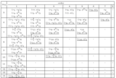
1 . Table

1.1 contains results of

computations made in the nineteenth century, for some particular

SL

2

-modules

(we use the notation

mVn

for the direct sum

L

m

i=1

Vn

of

m

copies of

Vn

).

The references [Bes69,

Ell95,

Gor69,

Gor87,

GY03,

Per87] give sets of generating

invariants of

mV

1

⊕

nV

2

in few particular cases, with small

m

and

n

. Gordan and

Grace & Young ([Gor75,

GY03]) gave an algorithm for computing the generators

of the covariants of

V

2

⊕

V

. Gordan ([Gor69,

Gor87]) gave good estimates on the

number of generators of the invariants of

nV

1

and of

V

1

⊕

nV

2

, with

n

≥

2 . Peano

(12)

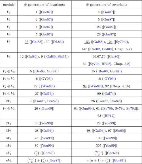
module #generators of invariants #generators of covariants V3 1 ([Gor87]) 4 ([Gor87])

V4 2 ([Gor87]) 5 ([Gor87])

V5 4 ([Gor87]) 23 ([Gor87])

V6 5 ([Gor87]) 26 ([Gor87])

V7 33 ([Gal88]), 30 ([DL86]) 153 ([Gal88]), 124 ([Sy79b]),

147 ([Crö02,Bed09], Chap. 5.7)

V8 12 ([Gal80]), 9 ([Gal80,Shi67]) 96,67,70 ([Gal80])

69 ([Sy79b,BB08], Chap. 5.8)

V2⊕V3 5 ([Bes69,Gor87]) 15 ([Bes69,Gor87])

V2⊕V4 6 ([GY03]) 18 ([GY03])

V2⊕V5 29 ( [Win80]) 94 ([Win80]), 92 (Chap. 5.16)

V2⊕V6 27 ([Gal74]) 99 ([Gal74]) 2V3 7 ([Gor87,Pea82]) 26 ([Gor87,Pea82])

V3⊕V4 20 ([Gun69]) 64 ([Gun69]), 61 ([Sy78b,Sy78c,Sy78d]),

63 ([BP12])

2V4 8 ([You99]) 28 ([You99]) 3V3 28 ([Gal94]) 98 ([Gal94]), 97 ([Sin05]) 3V4 25 ([You99]) 103 ([You99]) 4V4 80 ([You99]) 305 ([You99]) nV1 `n 2 ´ ([Gor69]) `n+1 2 ´ ([Gor69]) nV2 `n+1₂ ´+`n₃´([Gor87]) n(n+ 1) +`n₃´([Gor87])

Table 1.1: Cases treated in the 19th century (the underlined entries are results that

in the rst place turned out to be false and were later corrected)

of degree

≤

6 and order

≤

4 . Young ([You99]) showed that the covariants of

nV

4

, with

n

≥

5 , are generated by those of degree

≤

6 and order

≤

6 . These last

results were conrmed and proved with modern methods by Kraft & Weyman

([KW99]) in 1999. They are extended in Chap.

5 of this thesis: we give sets of

generating invariants for

mV

1

⊕

nV

2

,

mV

1

⊕

nV

3

, and

mV

1

⊕

nV

4

, with

m

≥

2 .

The diculty of nding generators of the algebra

I

of invariants is captured

by the homological dimension

hd

I

of

I

. If

r

is the minimal number of generators

of

I

, and

m

is the size of a system of parameters of

I

(set of algebraically

(13)

independent elements

P

1

, . . . , P

m

∈

I

such that

I

is integral over

C

[

P

1

, . . . , P

m

]

),

then

m

equals

n

−

2 for

n

≥

3 , and the homological dimension

hd

I

equals

r

−

m

([Pop83, Corollary 1]). Popov [Pop83] classied in 1983 all the

SL

2

-modules

V

n1

⊕

. . .

⊕

V

np

with

hd

I

≤

10 for a single binary form (

p

= 1

) and

hd

I

≤

3 for several binary forms (

p >

1 ). It turned out that all these cases

were known classically, as cases in which one could easily nd minimal sets of

generating invariants. Brouwer and I [BP11] extended Popov's classication

and determined for

p

= 1

the cases with

hd

I

≤

100 and for

p >

1 the cases

with

hd

I

≤

15 (see also Chap.

6 in this thesis). In the case of a single binary

form, the homological dimension

hd

I

rapidly increases if the degree is

≥

9 . The

bigger the homological dimension

hd

I

is, the harder it is to nd generating

invariants of

I

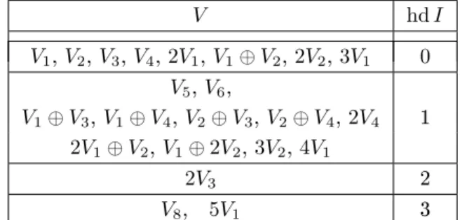
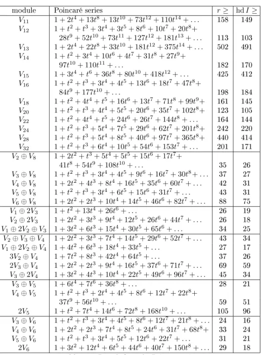
. The following table contains, for illustration, the values of

hd

I

for binary forms of degree less than 14:

degree

1

2

3

4

5

6

7

8

9

10

11

12

13 hd

I

0

1

25

3

85

98 ≥

149 ≥

103 ≥

491 r

1

2

4

5

30

9

92

106 ≥

158 ≥

113 ≥

502 With his book published in 1939 Weyl [Wey46] aimed to give a modern

introduction to the theory of invariants, translating the problem of nding the

generating invariants of binary forms into the language of representation theory

and the study of actions of the semisimple groups. He thought it was high time

for a rejuvenation of the classic invariant theory, which has fallen into an almost

petried state([Wey46]). Parshall [Par90] talks in 1990 about a myth saying

that

the death certicate of invariant theory eectively reads 15 February

1890. On that date, the twenty-eight-years-old David Hilbert signed

o his paper Über die Theorie der algebraischen Formen [Hil90] and

presented his proof of the so-called nite basis theorem to the

read-ership of the mathematische Annalen, a theorem and proof that

killed an entire area. Two and a half years later, he completed

yet another invariant-theoretic work, entitled Über die vollen

Invari-antensysteme [Hil93] and put an end to any lingering hopes of the

theory's resurrection. Thus, after fty years of vigorous life, one

of the nineteenth century's major areas of mathematical research

abruptly ceased to exist.([Par90])

This myth originated probably from Weyl's words on Hilberts papers:

His papers (1890/92) mark a turning point in the history of

invari-ant theory. He solves the main problems and thus almost kills the

whole subject. ([Wey46, page 27])

But we should note the words turning point and almost in Weyl's quote,

as Parshall [Par90] suggested. In the 1960's Mumford [Mum65] translated

pro-blems of invariant theory into the language of algebraic geometry. One of his

(14)

key insights was that one could analyse the geometry of group actions without

actually knowing the invariants. For instance, he proved that a vector in a

repre-sentation cannot be distinguished from zero by means of invariants if and only

if there is a one-parameter subgroup sending the vector arbitrarily close to zero.

The remarkable thing here is that a purely algebraic property (namely that all

non constant homogeneous invariants vanish on a vector) can be checked in a

purely geometric fashion (involving orbits of the vector under one-parameter

subgroups). As a consequence, we know for instance that all invariants of

bi-nary forms of degree

n

vanish on the forms having a root of multiplicity

>

n₂

without any a priori information on the invariants themselves. Mumford's

re-sult generalises Hilbert's criterion mentioned in Chap.

2.7.1, which will be used

throughout this thesis.

In the second half of the 20th century new techniques in commutative algebra

became available that can be applied to invariant theory. These techniques are

both of a theoretical nature, such as Hochster& Roberts's result that invariant

rings of reductive group representations are Cohen Macaulay [HR74], and of an

algorithmic nature, such as the use of Gröbner bases in invariant theory [DK00]

or the computation of Poincaré series of invariant rings [Spr77,

Bri82,

Bro94].

Such algebraic and algorithmic techniques are the starting point of this thesis.

This thesis is organised as follows.

In Chapter

2 we introduce the denitions and notations that will be used in

this thesis. In Chapter

3 we present the computational methods that we use for

nding the generating invariants of

SL

2

-modules. In Chapter

4 we nd the basic

invariants of

Vn

for

n

∈ {2

,

3 , . . . ,

10}

, and give explicit systems of parameters in

all these cases (Chap.

4.8 and

4.9 are joint work with Brouwer [BP10a,

BP10b]).

In Chapter

5 we review classical results regarding the invariants of

Vn

₁

⊕

. . .

⊕

Vn

_p

, with

p

≥

2 . We correct a result of Winter [Win80] on the generating

covariants of

V

2

⊕

V

5

(see Chapter

5.16) and results of Gundelnger [Gun69]

and Sylvester [Sy78b,

Sy78c,

Sy78d] on the generating covariants of

V

3

⊕

V

4

(see

Chap.

5.19, joint work with Brouwer [BP12]). In Chapter

6 we classify the

mo-dules

V

n1

⊕

. . .

⊕

V

np

whose algebras of invariants have a homological dimension

(15)

Chapter 2

Invariant Theory

2.1 Denitions and notation

Recall from the introduction the denition of the group

SL

2

. Denote by

Vn

the

space of binary forms of degree

n

.

Consider a rational, nite-dimensional

SL

2

-module

V

. Then there exist

(

n

1

, . . . , n

p

)

such that

V

'

V

n1

⊕

. . .

⊕

V

np

as

SL

2

-modules (cf. [Spr77, 3.2.2]).

The group

SL

2

acts on the algebra of polynomial functions on

V

n1

⊕

. . .

⊕

V

np

via

g

· j

(

f

1

, . . . , f

p

) =

j

(

g

−1

· f

1

, . . . , g

−1

· f

p

)

,

where

g

∈

SL

2

,

j

∈ O(

Vn1

⊕

. . .

⊕

Vn

p

)

and

(

f

1

, . . . , fp

)

∈

Vn1

⊕

. . .

⊕

Vn

p

.

Denition 2.1.1. Consider

V

=

V

n1

⊕

. . .

⊕

V

np

. An invariant of

V

is an

element

j

in the algebra

O(

V

)

of polynomial functions on

V

such that

g

· j

=

j

for all

g

∈

SL

2

. The set of invariants of

V

is denoted

O(

V

)

SL2

.

Example 2.1.1. Consider the binary form

f

=

a

0

x

2

+ 2

a

1

xy

+

a

2

y

2

∈

V

2

of

degree 2. The polynomial

j

(

f

) =

a

2

1

−

a

0

a

2

is an invariant of

V

2

.

Indeed, for

g

=

m np q

∈

SL

2

,

mq

−

np

= 1

, we have

g

· j

(

f

) =

j

(

g

−1

· f

)

and

g

−1

· f

=

a

0

(

mx

+

ny

)

2

+ 2

a

1

(

mx

+

ny

)(

px

+

qy

) +

a

2

(

px

+

qy

)

2

=

= (

a

0

m

2

+ 2

a

1

mp

+

a

2

p

2

)

x

2

+ 2(

a

0

mn

+

a

1

np

+

a

1

mq

+

a

2

pq

)

xy

+

+ (

a

0

n

2

+ 2

a

1

nq

+

a

2

q

2

)

y

2

.

It follows that

j

(

g

−1

· f

) = (

a

0

mn

+

a

1

np

+

a

1

mq

+

a

2

pq

)

2

−

(

a

0

m

2

+ 2

a

1

mp

+

a

2

p

2

)(

a

0

n

2

+

+ 2

a

1

nq

+

a

2

q

2

) = (

a

21

−

a

0

a

2

)(

mq

−

np

)

2

=

a

21

−

a

0

a

2

=

j

(

f

)

,

hence

g

· j

(

f

) =

j

(

f

)

for all

g

∈

SL

2

.

The invariant

j

has a geometric interpretation:

j

(

f

) = 0

if and only if

f

has a

double root.

(16)

Example 2.1.2. Let

f, `

∈

V

2

⊕

V

1

, with

f

=

a

0

x

2

+ 2

a

1

xy

+

a

2

y

2

∈

V

2

and

`

=

b

0

x

+

b

1

y

∈

V

1

. The polynomial

j

(

f, `

) =

a

0

b

21

−

2 a

1

b

0

b

1

+

a

2

b

20

is an

invariant of

V

2

⊕

V

1

. Indeed, for

g

=

m n p q

∈

SL

2

,

mq

−

np

= 1

, we have

g

· j

(

f, `

) =

j

(

g

−1

_·

_{f, g}

−1

_·

_`

₎

_and

g

−1

· f

= (

a

0

m

2

+ 2

a

1

mp

+

a

2

p

2

)

x

2

+ 2(

a

0

mn

+

a

1

np

+

a

1

mq

+

a

2

pq

)

xy

+

+ (

a

0

n

2

+ 2

a

1

nq

+

a

2

q

2

)

y

2

,

g

−1

· `

= (

b

0

m

+

b

1

p

)

x

+ (

b

0

n

+

b

1

q

)

y.

It follows that

j

(

g

−1

· f, g

−1

· `

) = (

a

0

m

2

+ 2

a

1

mp

+

a

2

p

2

)(

b

0

n

+

b

1

q

)

2

−

2(

a

0

mn

+

a

1

np

+

a

1

mq

+

a

2

pq

)(

b

0

m

+

b

1

p

)(

b

0

n

+

b

1

q

)+

+ (

a

0

n

2

+ 2

a

1

nq

+

a

2

q

2

)(

b

0

m

+

b

1

p

)

2

=

= (

a

0

b

21

−

2 a

1

b

0

b

1

+

a

2

b

20

)(

mq

−

np

)

2

=

j

(

f, `

)

,

hence

g

· j

(

f, `

) =

j

(

f, `

)

for all

g

∈

SL

2

.

The invariant

j

has a geometric interpretation:

j

(

f, `

) = 0

if and only if

`

and

f

have a common root.

Denition 2.1.2. Consider

V

=

V

n1

⊕

. . .

⊕

V

np

. A covariant of

V

of order

m

and degree

d

of

V

is an

SL

2

-equivariant polynomial map

φ

:

V

→

V

m

which

is homogeneous of degree

d

. In other words, for all

g

∈

SL

2

we have

φ

(

g

· v

) =

g

· φ

(

v

)

, where

v

∈

V

, and for all

t

∈

_C

we have

φ

(

tv

) =

t

d

_φ

₍

_v

₎

_{, where}

_v

_∈

_V

_.

The set of covariants of

V

is denoted

C(

V

)

.

Remark 2.1.1. The covariants of

V

of order 0 are the homogeneous

invari-ants of

V

. They form the homogeneous components of the ring

O(

V

)

SL2

₌

L

d

O(

V

)

SL2

d

of invariants of

V

, where

O(

V

)

SL2

d

are the invariants of

V

of

de-gree

d

. The covariants form a doubly graded ring

C(

V

) =

L

d,e

C(

V

)

(d,e)

, where

C(

V

)

(d,e)

are the covariants of

V

of degree

d

and order

e

.

Denition 2.1.3. For a covariant of

V

n

of order

m

and degree

d

we dene its

co-order to be

(

nd

−

m

)

/

2 .

The main way to construct covariants is via transvectants (Überschiebungen).

They are derived from the Clebsch-Gordan decomposition of the

SL

2

-module

Vm

⊗

Vn

, with

m

≥

n

:

Vm

⊗

Vn

'

Vm

+n

⊕

Vm

+n−2

⊕

. . .

⊕

Vm

−n

([

KP96

,

9 .

1])

.

This decomposition denes for each

p

,

0 ≤

p

≤

n

, an

SL

2

-equivariant linear map

Vm

⊗

Vn

→

Vm

+n−2p

, denoted

(

f, h

)

7→

(

f, h

)

p

, and called the p-th transvectant.

It is given explicitly by the following formula:

(

f, h

)

7→

(

f, h

)

p

:=

(

m

−

p

)!(

n

−

p

)!

m

!

n

!

p

X

i=0

(−1)

i

_p

i

_∂

p

_f

∂x

p−i

_∂y

i

∂

p

_h

∂x

i

_∂y

p−i

(2.1)

(17)

(see [Olv99, Chap. 5]). The maps

(

f, h

)

7→

(

f, h

)

p

are clearly bilinear. Also, if

f

=

`

m

1

and

h

=

`

n2

, with

`

1

=

a

0

x

+

a

1

y

and

`

2

=

b

0

x

+

b

1

y

, we have then

(

`

m₁

, `

n₂

)

p

=

`

m−p 1

`

n−p 2

[

`

1

, `

2

]

p

where

[

`

1

, `

2

] := det

a0a1 b0 b1

=

a

0

b

1

−

a

1

b

0

.

Furthermore, if

g

=

m np q

∈

SL

2

, with

mq

−

np

= 1

, we have

(

g

· `

m₁

, g

· `

n₂

)

p

= (

g

· `

1

)

m−p

(

g

· `

2

)

n−p

[

`

1

, `

2

]

p

(

mq

−

np

)

p

=

= (

g

· `

1

)

m−p

(

g

· `

2

)

n−p

[

`

1

, `

2

]

p

=

g

· (

`

m1

, `

n 2

)

p

.

Because

V

m

and

V

n

are linearly spanned by powers of linear forms, it

fol-lows that

(

f, h

)

7→

(

f, h

)

p

are

SL

2

-equivariant. They are also non-zero and

as

V

m+n

, V

m+n−2

, . . . , V

m−n

are irreducible representations, it follows that

Vm

⊗

Vn

→

Vm

+n

⊕

Vm

+n−2

⊕

. . .

⊕

Vm

−n,

(

f, h

)

7→

n

X

p=0

(

f, h

)

p

is surjective. But

Vm

⊗

Vn

and

Vm

+n

⊕

Vm

+n−2

⊕

. . .

⊕

Vm

−n

have the same

dimension, which implies that the map is actually a bijection.

Example 2.1.3. Let

f

=

a

0

x

3

+ 3

a

1

x

2

y

+ 3

a

2

xy

2

+

a

3

y

3

. The map

V

3

→

V

2

,

f

7→(

f, f

)

2

= 2(

a

0

a

2

−

a

21

)

x

2

_{+ 2(}

_a

0

a

3

−

a

1

a

2

)

xy

+ 2(

a

1

a

3

−

a

22

)

y

2

₌

=

1

18 [

∂

2

_f

∂x

2

∂

2

_f

∂y

2

−

(

∂

2

_f

∂x∂y

)

2

_]

_,

denes a covariant of

V

3

of order 2 and degree 2. Note that the transvectant

(

f, f

)

2

coincides, up to a constant, with the Hessian of

f

. This transvectant

vanishes if and only if

f

is the

3

th

power of a linear form (see Proposition

2.7.2).

Remark 2.1.2. The covariants of

V

can be identied with the invariants of

V

1

⊕

V

: we have

V

1

⊕

V

'

V

1∗

⊕

V

as

SL

2

-representations and the algebra of

covariants of

V

is isomorphic to

O(

V

₁∗

⊕

V

)

SL2

(see [Pro07, Chap. 15]). Each

covariant

φ

of

V

of order

m

corresponds to the invariant of

V

1

⊕

V

dened by

the transvectant

(

φ

(

v

)

, `

m

)

m

, where

`

∈

V

1

.

Notation agreement. Consider

f

∈

Vm

. One obvious covariant of

Vm

of

degree 1 and order

m

is the identity map on

Vm

. From now by the covariant

f

we will mean the identity map on

Vm

.

Given two covariants

φ

1

:

V

m

→

V

d

and

φ

2

:

V

m

→

V

e

of

V

m

of orders

d

,

re-spectively

e

, they dene the covariants

ψ

p

:

V

m

→

V

d+e−p

,

f

7→

(

φ

1

(

f

)

, φ

2

(

f

))

p

,

with

0 ≤

p

≤

min(

d, e

)

. By the covariant

(

φ

1

, φ

2

)

p

we will mean the map

V

m

→

V

d+e−p

,

f

7→

(

φ

1

(

f

)

, φ

2

(

f

))

p

.

(18)

Theorem 2.1.3. (Gordan [Gor68]) Let

f

∈

V

n

. Then, the covariants of

V

n

are generated by a nite number of iterated transvectants

f,

(

f, f

)

p

,

(

f,

(

f, f

)

p

)

q

, . . .

In particular (see [Gor68, 2]), if

C

is a covariant of

f

of degree

d

, then

C

can be written as a linear combination of transvectants

(

f, Ci

)

ri

, where

Ci

are

covariants of

f

of degree

d

−

1 .

This gives a method for nding the generating covariants of

f

: suppose

we know the generating covariants of

f

up to degree

d

−

1 . In order to nd

the generating covariants of degree

d

, we have to write down all transvectants

(

f, Cd

−1

)

r

, for suitable

r

, where

Cd

−1

is a covariant of degree

d

−

1 , namely a

generating covariant of degree

d

−1

or a product of total degree

d

−1

of generating

covariants of lower degrees. Then we select out of this set the irreducible ones

(we call a covariant

C

reducible if

C

is contained in the algebra generated by

all covariants of degree

≤

deg

C

and order

≤

ord

C

, where at least one of the

inequalities is strict).

Lemma 2.1.4. [KW99] Let

V

=

V

n1

⊕

. . .

⊕

V

np

be a representation of

SL

2

and

C

1

, . . . , Cr, C

covariants of

V

, of orders

ord

Ci

=

ei

. Then the

transvec-tant

(

C

1

. . . Cr, C

)

k

is reducible if there is a strict subset

S

⊂ {1

,

2 , . . . , r

}

and

integers

ki

≤

ei

such that

k

=

P

i∈S

ki

.

Proposition 2.1.5. Let

f

∈

Vn

and consider covariants

C

1

, . . . , Cr

of

f

, with

r

≥

2 . If the covariant

C

= (

C

1

. . . Cr, f

)

k

is irreducible, then

ord

C

≤

n

−

r

. If

n

is even, then

ord

C

≤

n

−

2 r

+ 2

.

Proof. Denote

mi

= ord

Ci

. W.l.o.g. we can assume

m

1

≥

m

2

≥

. . .

≥

mr

>

0 .

From the denition of transvectants,

k

must be

≤

n

. From Lemma

2.1.4 we

obtain:

m

1

+

m

2

+

. . .

+

m

r−1

< k

≤

m

1

+

m

2

+

. . .

+

m

r

.

Then,

ord

C

=(

m

1

+

m

2

+

. . .

+

m

r

) +

n

−

2 k

≤

≤(

m

1

+

m

2

+

. . .

+

mr

) +

n

−

2(

m

1

+

m

2

+

. . .

+

mr

−1

+ 1) =

=

n

−

(

m

1

−

mr

+ (

m

2

+

. . .

+

mr

−1

) + 2)

≤

n

−

r

If

n

is even, then all

m

i

will be even as well and then

n

−

(

m

1

−

m

r

+ (

m

2

+

. . .

+

m

r−1

) + 2)

≤

n

−

2 r

+ 2

.

Example 2.1.4. Consider

f

∈

V

1

. Then, we have

(

f, f

)

p

= 0

for

p

6= 0

. The

covariants of

V

1

are generated by

f

.

(19)

Consider

f

∈

V

2

. The covariants of

V

2

are generated by

f

and

(

f, f

)

2

; the

invariants of

V

2

are generated by

(

f, f

)

2

(see Chap.

4.1).

Consider

f

∈

V

3

. The covariants of

V

3

are generated by

f,

(

f, f

)

2

,

(

f,

(

f, f

)

2

)

1

,

((

f, f

)

2

,

(

f, f

)

2

)

2

=

−(

f,

(

f,

(

f, f

)

2

)

1

)

3

(see Chap.

5 .

3 .

1 ).

The invariants of

V

3

are generated by

((

f, f

)

2

,

(

f, f

)

2

)

2

(see Chap.

4.2).

Consider

f

∈

V

4

. The covariants of

V

4

are generated by

f,

(

f, f

)

2

,

(

f, f

)

4

,

(

f,

(

f, f

)

2

)

1

,

(

f,

(

f, f

)

2

)

4

(see Chap.

5 .

4 .

1 ).

The invariants of

V

4

are generated by

(

f, f

)

4

and

(

f,

(

f, f

)

2

)

4

(see Chap.

4.3).

For further examples see Chap.

4 and

5. Hilbert [Hil90] generalised Gordan's result to a system of several homogeneous

Invariants of binary forms

Invariants of binary forms

Inauguraldissertation

zur

Erlangung der Würde eines Doktors der Philosophie

vorgelegt der

Philosophisch-Naturwissenschaftlichen Fakultät

der Universität Basel

von

Mihaela Ileana Popoviciu Draisma

von Rumänien

auf Antrag von

Prof. Dr. Hanspeter Kraft und Prof. Dr. Jerzy Weyman

Basel, den 12. November 2013

Acknowledgments

I thank Hanspeter Kraft for trusting me with the study of invariants, for oering

me this work that gave me joy and inspiration, for his guidance and advice.

I thank Andries Brouwer for being such a nice and supportive collaborator and

co-author. It is a joy and an honour to work with him.

I thank Jerzy Weyman for the crash course on invariant theory he gave me in

the short moments we met in Basel and Boston.

I thank Varga Csaba, one of the brightest gures from my childhood and later

times. His maths circles were spots of light in the gray of communistic

school-time.

I thank my professors at Babes-Bolyai University and at Kaiserslautern

Univer-sity for the many inspiring lectures. I thank my colleagues and friends at the

Mathematical Institute Basel for the nice moments we had together.

I thank Renate and Hanspeter for hosting me in Basel whenever I came there

for working on my thesis, for listening to me, encouraging me, and supporting

me in their kind way. I thank them and my friends Joswitte, Simon, Regula,

Andreas, Jonas, Monika, Marine, Stéphane, Sebastian, Christoph, and Jaqueline

for making returning to Basel feel like returning to a second home.

I thank Oana, Catalin, and Marius for being such good friends, despite the

geographical distance. I thank my friends and relatives in the Netherlands for

their support.

I thank my parents, especially my mother, for unconditionally coming to help

me whenever I need.

I thank Jan and Mirona for making my days so bright.

Contents

1 Introduction

7

2 Invariant Theory

15

2.1 Denitions and notation

. . . 15

2.2 The symbolic method

. . . 19

2.3 Bounds on the degrees and orders of the generating covariants

. . 22

2.4 Cohen-Macaulayness

. . . 25

2.5 The Poincaré series

. . . 27

2.5.1 A result of Broer and Poincaré series

. . . 29

2.6 The quotient variety and nullforms

. . . 30

2.7 Finding a hsop

. . . 31

2.7.1 Hilbert's criterion

. . . 31

2.7.2 Dixmier's criterion

. . . 33

2.8 Schur modules

. . . 34

2.9 The type of the generating covariants

. . . 37

3 Computational methods

39

3.1 The method

. . . 39

3.2 The computation of invariants and covariants

. . . 40

3.3 The computation of the Poincaré series

. . . 40

3.4 Linearly independent invariants

. . . 42

3.5 The example of the binary octavic

. . . 43

4 Invariants of binary forms