UIUC Technical Report: UIUCDCS-R-2007-2911. October 2007
Contextual Indexing and Joining:
Supporting Efficient, Scalable Entity Search
Tao Cheng and Kevin Chen-Chuan Chang
Computer Science Department University of Illinois at Urbana-Champaign
{
tcheng3,kcchang
}@cs.uiuc.edu
ABSTRACT
As the Web has evolved into an entity abundant repository, with the standard “page view”, current search engines are becoming increas-ingly inadequate for a wide range of query tasks. Entity search, a significant departure from document retrieval, finds fine granular-ity information, i.e., entities, embedded in documents directly and holistically across the whole collection. Essentially, entity search is to find matching entities by context patterns from each document and to aggregate them across documents for ranking. This text-based pattern matching suggests that standard inverted lists-text-based query processing can be applied. However, this baseline is lim-ited in both efficiency, due to long entity lists, and scalability, due to cross-document aggregation. To enhance efficiency, we propose “contextual index”, an index that materializes pre-joins, to elim-inate unnecessary index reading and reduce online matching. To improve scalability, we propose “entity-space” partitioning, so that answer subspaces can be aggregated locally. We reason our design rationale from both the functional and the operational definition of entity search, and show that they consistently reach our framework. We evaluate the indexing (contextual indexing) and parallel query processing (contextual joining) framework over a 2TB real Web corpus with systematic benchmark query sets. Experiments show that our scheme can speed up query processing by, in average, two order of magnitude over the baseline.
1.
INTRODUCTION
The immense scale and wide spread of the Web has rendered it as an ultimate information repository– as not only the sources where we find but also the destinations where we publish our information. These dual forces have enriched the Web with all kinds of data, much beyond the conventional page view of the Web as a corpus of HTML pages, or “documents.” Consequently, the Web is now a collection of data-rich pages, on the “surface Web” of static URLs (e.g., personal homepages) as well as the “deep Web” of database-backed contents (e.g., flights from aa.com). While the richness of data represents a promising opportunity, it challenges us for effec-tively finding information we need.
With the Web’s sheer size, our ability to find “stuff” we want mainly relies on how search engines respond to our queries. As
.
current engines search the Web inherently with the conventional page view, they are becoming increasingly inadequate for a wide range of queries. To focus on the “stuff” we want, or data “enti-ties”, as many recent efforts also aim at (e.g., [4, 5, 17, 15, 13, 12, 1, 2, 3, 14, 19]), we have proposed the notion of entity search over a corpus of text documents (such as the Web), in terms of its rank-ing function [7] and its applications in information integration [6]. Upon this foundation, to realize ad-hoc entity search over a large corpus, this paper studies the key challenges of query processing.
As the Web is rich with various type of data, users are often looking for specific “fine grained” information, or data objects of specific types, each of which we call an entity. The notion of en-tity can broadly refer to anything that can be reasonably recognized from the text corpus, either straightforwardly or with sophisticated techniques, often with uncertainty (see Section 2). To motivate, consider user Amy: She may be looking for the “phone number” of say, Amazon.com’s customer service? To apply for graduate school, how can she find the list of “professors” in the database area? When preparing seminar presentation, Amy wants to find papers that come readily with presentations, i.e., a “PDF file”
to-gether with a “PPT file,” say from SIGMOD 2006? Or, to buy
Shakespeare’s Hamlet, how can she find the “prices” and “cover images” of available choices from, say, Borders.com and BN.com? In these scenarios, like every user in many similar situations, Amy is looking for particular entities of information, e.g., a phone number, a book cover image, a PDF, a PPT, a name, a date, an email address, etc. We thus aim at supporting entity search, to directly find matching entities across as many pages as they may occur. To illustrate, our scenarios will lead to the following queries:
Q1:ow20(amazon service#phone)
Q2: (#professor#university#research=”database”)
Q3: ow(sigmod 2006#pdf file#ppt file)
Q4: (#title=”hamlet”#image#price)
First, as input, users formulate queries to directly describe what they are looking for: She can simply specify what her target entities are and what keywords may appear in the surrounding “context” with a right answer. To distinguish entities and keywords, we use a prefix #, e.g., #phonefor the phone entity. Each query is thus essentially a context pattern of how the desired entity may occur with some keywords in its surrounding context. Q1says that the entity#phonewill appear with these keywords in the pattern of
ow20or “ordered-window of 20 words” (and as close as possible). We may also omit the window size (e.g.,Q3, which is default to 100 words window) or even the entire pattern, e.g.,Q2andQ4, in which case the implicit defaultuwor “unordered-window” is used (which means proximity– the closer in a window, the better). The exact patterns depend on implementations.
Second, as output, users will directly get their desired entities. That is, as a query specifies what entity types are the targets, its
… … … … hp.com 0.2 206-346-2992 4 xyz.com 0.6 800-342-5283 3 Dell.com/supportors 0.8 800-988-0886 2 amazon.com/support.htm myblog.org/shopping 0.9 800-201-7575 1 urls score phone number rank … … … … … ms.com 0.7 surajit21.ppt surajit21.pdf 2 db.com,sigmod.com 0.8 sigmod6.ppt sigmod6.pdf 1 urls score PPT PDF rank
Figure 1: Query Results ofQ1andQ3
results are those entity instances (or literal values) that match the query, in a ranked order by their matching scores. Figure 1 shows some example results forQ1andQ3.
Third, as search mechanism, entity search will find matching en-tities holistically, where an instance will be found and matched in all the pages where it occurs. For instance, a#phone 800-201-7575 may occur at multiple URLs as Figure 1 shows. For each instance, all its matching occurrences will be aggregated to form the final ranking– e.g., a phone number occurs more frequently at where “amazon customer service” is mentioned may rank higher than those less frequent ones. Thus, while our search target is enti-ties, as supporting “evidences,” entity search will also return where each entity is found. Users can examine these snippets for details.
We note that, the usefulness of entity search is three-fold, as the sample results in Figure 1 illustrate. First, it returns relevant an-swers at top rank places, greatly saving search time and allowing users or applications to focus on top results. Second, it collects all the evidences regarding the query in the form of listing supporting pages for every answer, enabling results validation (by users) or program-based post-processing (by applications). Third, by target-ing at typed entities, such an engine is data-aware and can be inte-grated with DBMS for building novel information systems– imag-ine the results ofQ1toQ4are connected with SQL-based data.
Toward supporting such entity search, there are several open is-sues we must address. To begin with, how to effectively score and rank entities? As we studied in [7], there are several unique re-quirements. Entity search is 1) contextual, as it is mainly matching by the surrounding context; 2) holistic, entities must be matched across their multiple occurrences over different pages; 3)
uncer-tain, since entity extraction is imperfect in nature; 4) associative,
entities can be associated in pairs, e.g.,#phoneand#emailand it is important to tell true association from accidental; and 5)
dis-criminative, as entities can come from different pages, and not all
such “sources” are equivalent. As a foundation, we have developed EntityRank and demonstrated its effectiveness in [7].
This paper focuses on the ensuing challenge for online entity search, how to support efficient and scalable query processing? While we started with extending standard document search in a “natural” way (Section 2), which indexes entities in the same way as keywords in inverted lists, we found this baseline, calledBasic, quite inadequate: First,Basic is inefficient because of the lengthy lists of entities. Note that each entity (e.g.,#phone) is not a unique literal value, unlike a keyword; instead, it is a large set of instance values (e.g., the numerous phone numbers on the Web). The extremely-long inverted lists of entities thus dominate and slow down query processing. Second,Basic is non-scalable, because it parallelizes by partitioning the document space. Such partitioning, while nat-ural for page search, does not amortize computation to the local nodes in a cluster, and thus leaves the central node as the bottle-neck. This paper proposes our solutions, which addresses the issue of 1) index design, for which we develop contextual index, and 2) data parallelization, for which we develop partitioning by entity
space. Amazon customer service 800-201-7575 [email protected] Amazon service 800-322-9266 Ebay Amazon customer service 800-201-7575 … … 6 d 9 d 97 d } :# , :# {E1 phoneE2 email E= 800-322-9266 p86 …… … …… … 800-201-7575 p8 …… … phone E :#1 service@ amazon.com e81 …… … …… … abc@ xyz.com e1 email E2:# ) (# phone I (amazon I 0.9 p10 323 d2 … … … … 0.9 p86 45 d9 0.8 p8 50 d97 … … … … 0.8 p8 23 d2 conf inst pos docid } ,..., {d1 d100 D= 55 d56 5 d64 34 d9 257 d9 45 d97 17 d6 12 d2 pos docid
Page View Entity View
Entity Instances Occurrence Relations
Entities Keywords ) (# email I … … … … … … … … … … … 1.0 e81 27 d6 conf inst pos docid … …
Figure 2: A running example:YellowPage.
Our results show that contextual indexing and its data paralleliza-tion is quite efficient: In our prototype indexing 2 TB of real Web corpus (with 90+ million pages), across a cluster of 34 nodes, for aYellowPage setting (similar to that of queryQ1), we systemat-ically queried a sample of Fortune-500 companies and SIGMOD 2007 PC members, with varying number of keywords and entities. Our contextual-index approach constantly and significantly outper-forms theBasic baseline of current document-based search, with an average of 200 - 500 times speedup, or over two orders of magni-tude faster. In terms of absolute time, the speedup reduces response time from, in average, 11.5 seconds (ofBasic) to 0.09 second (of our scheme), thus in effect making on-line query processing possi-ble. We note that the speedup is constant across our analysis with respect to the number of keywords, the number of entities, and the “selectivity” of context pre-joining, as Section 5 will report.
We start in Section 2 to formalize entity search and its chal-lenges. Section 3 proposes our solution, for which Section 4 con-cretely develops its realization. Section 5 reports our prototype sys-tem and experiments, and we relate to existing studies in Section 6.
Contributions
1. As the foundation for abstracting the computation of entity search, we identify its operational definition. (Section 2)
2. We develop index design and data parallelization for query processing, reasoning from both the functional and operational perspectives of entity search. (Section 3, 4)
3. We have implemented the contextual index-based entity searcher in an online prototype with real Web corpus, and demonstrated the effectiveness and efficiency of entity search.
2.
THE PROBLEM: ENTITY SEARCH
We now define entity search, and identify its challenges in query processing. We will discuss from dual perspectives: First, to see the “semantics” of entity search, we will examine the functional perspective, in terms of how the output is related to the input (Sec-tion 2.1). Second, to understand its computa(Sec-tion, the focus of this paper, we will develop the operational perspective (Section 2.2). Together, they will lead us to identifying the challenges in query processing (Section 2.3). The dual perspectives will further inspire consistent insights for a solution, which Section 3 will present.
For our discussion, we will use Figure 2 as a running example, which we call theYellowPage scenario, as it provides search for contact information#phoneand#email. As a toy dataset, the cor-pusDhas 100 documentsD = {d1, . . . , d100}; we show three documentsd6, d9,d97as examples. (The scenario is indeed our experimental setting, in which we indexed 90+ million pages.) We will also assumeQ1(Section 1) as the query.
2.1
Entity Search: Functional Definition
To understand its semantics, we define entity search from aData Model: To view the Web as a repository to search over, in
contrast to page-oriented search, where the Web is a set of docu-ments (or pages)D={d1, . . . , dn}, we take an entity view, which considers the Web as primarily a repository of entities (which ap-pear over pages): E = {E1, . . . , EN}. The set of entity types
Eito support depends on the search applications (much like the “schema” of a database application defines attributes to use). E.g., to support Scenario 1 (Section 1), i.e., ourYellowPage setting (Fig-ure 2), the system might be constructed with entitiesE = {E1 :
#phone, E2:#email}. In [7], we presented several applications of
entity search with various schemas.
Each entityEiis a set of entity instances{ei1,. . .,eih}that are extracted from the corpus, i.e., literal values of entity typeEithat occur somewhere in somed∈D. We useeito denote an entity in-stance of entity typeEi. In the example of phone-number patterns, we may extract#phone={“800-201-7575”, “244-2919”, “(217) 344-9788,. . .}. As Figure 2 shows, forYellowPage,#phoneis a set of 100 distinctive phone entity instances{p1, . . . , p100}and#email is a set of 100 distinctive email entity instances{e1, . . . , e100}.
These entities are recognized offline, and their instances are in-dexed for efficient search– which is the focus of this paper. For en-tity extraction, we can adopt a range of existing techniques: from simple file types (e.g., for#pdf, #ppt), dictionaries (e.g., #state,
#professor,#senator), pattern matching (e.g.,#phone,#email), to
state-of-the-art named-entity taggers (e.g., entityname,# organiza-tion). Our system description [8] discusses our current implemen-tation of entity extraction.
To enable query matching in search, for each entity instancee(of typeEi), e.g.a particular#phone(say, 217-321-1234), as it may oc-cur many times, we will record all its ococ-currences across documents inD. At offline indexing time, by scanning throughD, each
occur-rence of an entity instance will be recognized by entity extraction
(as just explained). For each occurrenceo, we record certain
prop-erties (or “features”) that characterize whatois, in order for online matching with queries. While the exact choice of features depend on the ranking algorithm, they must capture the appearance, con-fidence, and position of each occurrence. For concrete discussion, without loss of generality, we assume the following simple proper-ties, which our ranking modelEntityRank [7] actually uses. • Where doesooccurs? As the position,o.docidis a document id
ando.attrpos a word offset of occurrence.
• What instance doesorepresent? As the instance,o.instis of the formEi.eindicating an instance idewith respect to type idEi. • How certain is the extraction? Confidenceo.confis an
probabil-ity estimation given by the entprobabil-ity extractor.
Our entity view thus considers the extraction ofEi overD as a
relation (i.e., a set of tuples, each with the above fields) of allEi occurrences. (As we will see in the operational perspective, consid-ering the entity view as “relational” enables us to defines operations algebraically.) EachEithus induces an occurrence relationI(Ei) as follows, e.g.,I(#phone)forYellowPage, as in Figure 2.
I(Ei) ={ohdocid,pos,inst,confi,s.t.ooccurs inD, o.inst ∈Ei.}
Meanwhile, keywords remain essential, as they are used to match with entities, much like their role in document search. Like enti-ties, each keywordkj, say “amazon,” can occur many times inD, which we also record in a similar occurrence relation. However, unlike entities, each occurrencexofkj is a literal value of itself without multiple different instances, and it can be recognized with-out uncertainty. Thus, the occurrence relation ofkjis of a simpler form, e.g.,I(amazon)forYellowPage (Figure 2).
I(kj) ={κhdocid,posi,s.t.ooccurs inD}
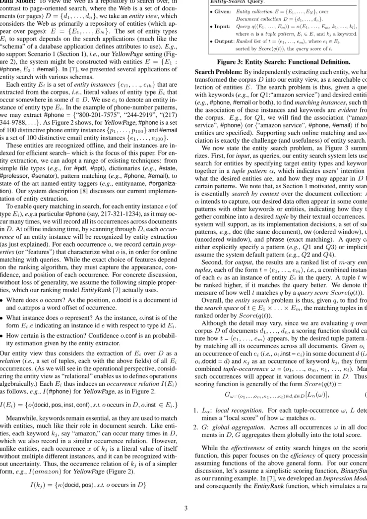
Entity-SearchQuery.
•Given: Entity collectionE={E1, . . . , EN}, over
Document collectionD={d1, . . . , dn}.
•Input: Queryq(hE1, . . . ,Emi) =α(E1, . . . ,Em,k1,. . .,kl),
whereαis atuple pattern,Ei∈E, andkja keyword.
•Output:Ranked listoft=he1,. . .,emi, whereei∈Ei,
sorted byScore(q(t)), thequery scoreoft.
Figure 3: Entity Search: Functional Definition. Search Problem: By independently extracting each entity, we have
transformed the corpusDinto our entity view, as a searchable col-lection of entitiesE. The search problem is thus, given a query with keywords (e.g., forQ1:“amazon service”) and desired entities (e.g.,#phone,#emailor both), to find matching instances, such that the association of these instances and keywords are evident from the corpus. E.g., for Q1, we will find the association h“amazon service”,#phonei(orh“amazon service”,#phone,#emailiif both entities are specified). Supporting such online matching and asso-ciation is exactly the challenge (and usefulness) of entity search.
We now state the entity search problem, as Figure 3 summa-rizes. First, for input, as queries, our entity search system lets users search for entities by specifying target entity types and keywords together in a tuple patternα, which indicates users’ intention of what the desired entities are, and how they may appear inDby certain patterns. We note that, as Section 1 motivated, entity search is essentially search by context over the document collection: As
αintends to capture, our desired data often appear in some context patterns with other keywords or entities, indicating how they to-gether combine into a desired tuple by their textual occurrences. A system will support, as its implementation decisions, a set of such patterns, e.g.,doc(the same document),ow(ordered window),uw
(unordered window), and phrase(exact matching). A query can either explicitly specify a pattern (e.g.,Q1andQ3) or implicitly assume the system default pattern (e.g.,Q2andQ4).
Second, for output, the results are a ranked list ofm-ary entity
tuples, each of the formt=he1,. . .,emi, i.e., a combined instance of eacheias an instance of entityEiin the query. A tupletwill be ranked higher, if it matches the query better. We denote this measure of how welltmatchesqby a query scoreScore(q(t)).
Overall, the entity search problem is thus, givenq, to find from the search space oft∈E1×. . .×Em, the matching tuples in the ranked order byScore(q(t)).
Although the detail may vary, since we are evaluatingqover a corpusDof documentsd1,. . .,dn, a scoring function should cap-ture howt=he1,. . .,emiappears, by the desired tuple patternα, by matching all its occurrences across all documents. Givenoias an occurrence of eachei(i.e.,oi.inst=ei) in some documentd(i.e.,
oi.docid=d) andκjas an occurrence of keywordkj, they form a
combined tuple-occurrenceω= (o1,. . .,om,κ1,. . .,κl). Many such occurrences will appear in various document inD. Thus a scoring function is generally of the formScore(q(t)) =
Gω=(o1,...,om,κ1,...,κl)∈d,d∈D[Lα(ω)], (1)
1. Lα: local recognition. For each tuple-occurrenceω,L deter-mines a “local score” of howωmatchesα.
2. G: global aggregation. Across all occurrences ωin all docu-ments inD,Gaggregates them globally into the total score. While the effectiveness of entity search hinges on the scoring function, this paper focuses on the efficiency of query processing, assuming functions of the above general form. For our concrete discussion, let’s assume a simplistic scoring function,BinarySum, as our running example. In [7], we developed an Impression Model, and consequently theEntityRank function, which simulates a
ran-S
scoreI(E1)
Lαααα
I(Em) I(k1) I(kl) ((((E1,...,Em))))GGGGG(((( ))))wasscore
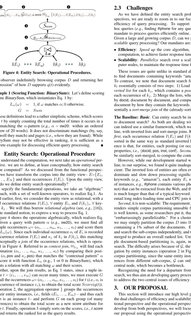
Figure 4: Entity Search: Operational Procedures.
dom observer indefinitely browsing corpusD and returning her “impression” of howDsupportsq(t) evidently.
Example 1 (Scoring Function:BinarySum): Let’s define scoring
schemeBinarySum, which instantiates Eq. 1 by:
Lα(ω) = 1,ifωmatchesα; 0otherwise.
G = Sum
These definitions lead to a rather simplistic scheme, which scores tupletby simply counting the total number of times it occurs in a way matching theα-pattern (e.g., α=ow20: within an ordered window of 20 words). It does not discriminate matchings (by, say,
how well they match) and pages (i.e., where they are found). While
BinarySum may not be effective in ranking, it is sufficient as a concrete example for discussing efficient query processing.
2.2
Entity Search: Operational Procedure
To understand the computation, we next take an operational per-spective. we are to define, at least conceptually, how entity search can be computed? As we discussed from the functional perspec-tive, we have transform the corpus into the entity view–E={E1,
E2,. . .,EN}and their occurrencesI(Ei). Upon the entity view, how do we define entity search operationally?
To sepcify the fundamental operations, we take an “algebraic” approach, with a set of well-known operators, to realize Eq.1. As stated earlier, first, we consider the entity view as relational, with a set of occurrence relationsI(Ei),∀entityEi, andI(kj),,∀ key-wordkj. We will thus borrow relational algebra (see, e.g., [16]), a quite standard notion, to express a way to process Eq. 1.
Figure 4 shows the operations algebraically, which realizes Eq. 1. Given a query with patternα(e.g., ow20), we must find all the tuple occurrencesω= (o1,. . .,om,κ1,. . .,κl) and score them withLα(ω). Since each individual occurrenceoiofEiis recorded in occurrence relationI(Ei)andκjofkjinI(kj), this matching is conceptually a join of the occurrence relations, which is opera-tion 1 in Figure 4. Referred to as context join,1Lαwill find each
combination (o1, . . ., om, κ1, . . ., κl) by comparing their posi-tions (oi.posandκj.pos) that matches the “contextual pattern”α
and score it with functionLα(e.g., 1 or 0 inBinarySum), which outputs a relation with all matchingωand their scores.
Further, upon the join results, as Eq. 1 states, since a tuple in-stancet=he1,. . .,emican occur many times, we must executeG over all the occurrencesω= (o1,. . .,om,κ1,. . .,κl) fort(i.e.,oiis an occurrence of instanceei), to obtain the total scoreScore(q(t)). In operation 2, the aggregation operator}groups the occurrences by their entity instances, i.e., fields (E1,. . .,Em) – and thus each group is an instancet– and performGon each group (of many occurrences) to obtain the total score as a newscoreattribute for groupt. Finally, operation 3 simply sorts on the scores, i.e.,t.score
∀t, and returns the ranked list as the query results.
2.3
Challenges
As we have defined the entity search problem from both per-spectives, we are ready to zoom in to our focus in this paper– the efficiency of query processing. To support entity search for ad hoc queries (e.g., finding#phonefor any query keywords), it is a mandate to process queries efficiently online. Our challenges are– Given a large and growing corpusD, can we perform efficient and
scalable query processing? Our mandates are:
• Efficiency: Speed up the core algorithm, in terms of I/O and
computation, to achieve faster response time.
• Scalability: Parallelize search over a scalable cluster of
com-puter nodes, to maintain the response time for growing corpus. These issues are quite unlike in standard document search, say, to find documents containing keywords “amazon” and “service.” To contrast, we note that document search for keywordsk1,. . .,
klessentially consists of two steps: 1) Load into memory the
in-verted list for eachkj, which contains a postinghdocid,posifor each occurrence ofkj. 2) Merge the lists, which are already sorted
bydocid, document by document, and compute the score for each
document by how they contain the keywords. Note this step is es-sentially a sort-merge join of the (already-sorted) lists.
The Baseline:Basic. Can entity search be implemented similarly
to document search? As both are dealing with text, entity search can indeed use a similar framework, which we call theBasic base-line, with inverted lists and sort-merge joins. Referring to Figure 4,
first, each occurrence relationI(Ei)andI(kj)can be stored and sorted in the same way as standard inverted lists; the only differ-ence is that, for entities, each posting (or occurrdiffer-ence)ohas more properties, i.e.,hdocid,pos,inst,confi. Second, these lists can then
be similarly sort-merged, to compute the context joinLα. However, while our development started with this simple base-line, to our surprise, we found it quite inadequate: First, it is ineffi-cient: The inverted lists of entities are often extremely long, which dominate and slow down processing significantly. Unlike literal keywords (e.g., “amazon”), each entityEi represents a large set of instances, e.g.,#phonecontains various phone numbers (true or not) that can be extracted from the Web, and thus its listI(#phone)
is much longer than that of a typical keyword. Such a long list will entail long index loading time and CPU join time.
Second, it is non-scalable: The requirement group-and-aggregation
renders simple corpus partitioning unusable for parallelization. It is well known, as some researchers put it, that document search is “embarrassingly parallelizable.” For a cluster of, say, 100 nodes, we may simply partition the corpusDinto 100 sub-corpora, each containing a 1% subset of the documents. Each node will index and search the sub-corpus independently, and the results are simply merged to produce an overall ranked list. Unfortunately, this sim-ple document-based partitioning is, again, not suitable for entity search. The difficulty arises because ofG, the grouping and aggre-gation by entity instances (operation 2 in Figure 4). With simple corpus partitioning, since the same entity instance can have occur-rences from different sub-corpus, G can only be performed at a central node, which becomes a bottleneck.
Recognizing the need for a departure from standard document search, we thus aim at developing query processing for entity search, to address the two central issues of efficiency and scalability.
3.
OUR PROPOSAL
This section will introduce our high level proposal to deal with the dual challenges of efficiency and scalability from both the func-tional perspective and the operafunc-tional perspective. While we try to develop from both perspectives, we will focus more concretely on our proposal using the operational perspective, since it is directly
Search Space Matching Pattern
Document Search d∈D={d1,. . .,dn} kjind’scontent
Entity Search t∈E1× · · · ×Em kjint’scontext
Figure 5: Contrast: Entity Search vs. Document Search.
the computation model ( 4). However, as we will show in this sec-tion, the two perspectives lead to the same solution.
We now propose our solution for an entity searcher. As Sec-tion 2.3 explained, the challenges of efficiency and scalability arise from two central issues, which our entity searcher must address. I1. How to indexI(Ei)andI(kj)? In baselineBasic, adapting
in-verted lists results in long entity listsI(Ei), which dominate and slow down query processing.
I2. How to partition the corpus? In the baseline, document-based partitioning renders aggregation a central bottleneck.
Parallel to the dual perspectives, functional and operational, of defining entity search (Section 2), we will also derive from the two aspects, in Section 3.1 and 3.2. It is interesting to note that, from not only the functional nature but also the computation aspect, we obtain the same conclusion.
3.1
Functional Perspective
From the functional perspective, we would like to reason from the nature of the search problem, as Section 2.1 defines. Unlike the direct adaptation inBasic, we wish to draw deeper insights from document search, to parallel our design of an entity searcher with that of a document searcher.
As Section 2.1 defines (Figure 3), given queryα(E1, . . . ,Em,
k1,. . .,kl), an entity searcher must find entity instancesthe1,. . .,
emi, from the spaceE1× · · · ×Em, that match those keywords in their context (e.g., #phone around the mentions of “amazon” and “service”). In contrast, for document search, a similar query finds documents from the spaceD={d1, . . .,dn}by matching keywords in their contents (e.g., documents containing “amazon” and “service”). Figure 5 highlights these contrasts in search space and matching pattern. With these contrasts, we can parallel our design with document search, reaching two design principles:
Principle A1: Indexing by Inverting to Entities via Context.
Observe that, for document search, an inverted list for keywordk
is an inversion fromkto each documentd∈D, wherekoccurs within its content, or, in short, indexing by inverting to documents
via content. Generalizing this observation, as we are now searching
for entities as targets, by keywords in their context, our indexes shall be the inversions from keywords to each instanceei ∈Ei, wherekoccurs around its context. (How to define this “context”– such as a certain-sized window, is an implementation decision.)
Principle A2: Parallelizing by Partitioning the Entity Space.
Observe that, for document search, the parallelization scheme nat-urally partitions the search spaceDinto disjoint subsetsD1,. . .,
Dn, i.e.,D1∪. . .∪Dn =DandDi∩Dj =∅. As our search target now is entities, applying the same principle, we should par-allelize by partitioning the space of each entityEiinto non-disjoint subsetsEi1,. . .,Eins.t.Ei1∪. . .∪Ein=EandEij∩Eik=∅.
3.2
Operational Perspective
Will our conclusion be the same, if we reason from the opera-tional perspective? As Section 2.2 discusses (which Figure 4 sum-marizes), entity search computationally consists of join, aggrega-tion, and ranking. From the perspective of speeding up and paral-lelizing this process, we will reach the following two principles:
Principle B1: Indexing by Pre-Computing Context Joins. To
speed up, as the inefficiency lies in the lengthy entity listsEi, the remedy is naturally to perform pcomputation, and build the re-sults into indexes. What pre-computation will speed up the context-join 1Lα(I(E1), . . ., I(Em), I(k1), . . ., I(kl))? Clearly, any
sub-joins will help. E.g., with sub-joinCa#p=1α(I(amazon),
I(#phone)) materialized, for queries likeQ1we can merge this
re-sult with the missing components to produce the overall join, i.e.,
1α(I(amazon),I(service),I(#phone)) =1α(Ca#p,I(service)).
Why is this more efficient? By pre-joining “amazon” and#phone,
Ca#pnot only contains all the necessary instances of both, but also
prunes out many “unmatched” ones, thus reducing both index load-ing and joinload-ing time. This principle speeds up full joins by materi-alizing some or all parts of it, and build the “sub-joins” into indexes. Note that, in pre-computation, we are concerned with only match-ing patternsα; the actual scoring byLshould only be executed in the final full joins. Thus, to simplify discussion, we will only show patterns in joins here. Further, since we want to build materialized sub-joins for as many queries as possible, we should execute prun-ing by a super pattern (e.g.,α∗=w100, or within 100-word win-dow of proximity) which will subsume any patterns that the system supports (e.g.,α=ow20as inQ1; i.e.,α→α∗
). The choice of the super pattern depend on implementation.
To understand the design issues of what sub-joins to materialize, we look further into how they may help with query processing: Let’s denote a (full or partial) context-join as1α∗(I), whereI
is the set of (entities or keyword) occurrence relations covered in the join; i.e.,Ca#phasI={I(amazon),I(#phone)}. Note that
the individual occurrence relation, such asI(amazon), is thus a special case where|I|= 1, representing a basic inverted list. We can state how sub-joins contribute as follows:
1α(I) = 1α[1α∗ (I1), . . . ,1α∗(In)], (2)
if I=∪(I1, . . . ,In).
Considering each sub-joins as a view, the choices of views to materialize is thus the issue of view materialization (e.g., [20, 11]) for answering future queries. While the exact choices will depend on the expected query workloads, entity search has certain char-acteristics that simplify this decision. First, like document search, entity-search queries also tend to be simple: In terms of entities, queries with one entities are common, while three or more entities are rare; in terms of keywords, as in traditional keyword queries, the average query length will be below 3. Second, the simplest query possible has one keyword (to match with) and one entity (to search). With these observations, we shall pre-compute for sim-ple “sub-joins” with one keyword and one entity. At run time, by applying Eq. 3, we can assemble these simple sub-joins for any queries that contain them. E.g.,Ja#pwill also be useful for other
queries (amazon books#phone) or (amazon#phone#email). Concretely, we propose to pre-join only pairs of keywords and entities: We will build contextual index, by context-joining every pair of one keywordkjand one entityEi:
C(kj, Ei) =1α∗ [I(kj), I(Ei)] ∀Ei,∀kj. (3) Remark: Principle B1 is consistent with A1. Observe that, each
contextual indexC(kj, Ei)associateskjwithEi, when they to-gether match a context patternα∗. From the standpoint of keyword
kj, the contextual index is to find all entity instances, in whose con-textkjappears– Thus clearly, it is indeed an inversion fromkjto entities via a context pattern.
Principle B2: Parallelizing by Partitioning along Groups. To
parallelize the join-aggregation-ranking process in Figure 4, since the final ranking must be performed to the overall results, it must
remain at the central node, and thus our objective is to “push down” the aggregationGto be executed at each local node. AsGperforms aggregation (by functionG) for each group of the same entity in-stances, to push it down to a local node, we must make sure that each node has an entire group forhe1,. . .,emi. Thus, this princi-ple suggests partitioning along groups.
Since we have proposed using contextual indexes, as Eq. 4 de-fines, our issue is now how to partition these indexes. (These lists will be stored by extending the structure of inverted lists; see Sec-tion 4.) For a contextual indexC=C(kj, Ei), how to partition it? To partition along the groups, we make sure the same instances of
Eiwill be allocated at the same local node, which means we must divideEiinto subsets. Specifically, we partitionEitonnodes, i.e.,
Ei=∪(Ei1,. . .,Ein), and consequently the partition of contextual indexCfollows: We can compute the sub-indexCzby pre-joining only the entity subsetEz
i, or simply computingConce and “pro-jecting” it to the subset, as follows:
Cz=C(kj, Eiz) = 1α∗ [I(kj), I(Eiz)] =C|Ez
i (4)
This partition, by dividing contextual indexes, is best suited for the common cases of simple queries. For queries with one entity (e.g.,Q1), say Ei, this scheme gives highly parallel processing. Since each tupletcontains just an instance ofEi(i.e.,t=heii, for
ei∈Ei), the corresponding group is fully contained in the local node whereeiis allocated to, and thus the aggregationGcan in-deed be pushed down fully, leaving only ranking at the central node. Section 4 will present the detail. For queries with multiple entities (e.g.,#phoneand#email), as each group is for a composite instance he1,. . .,emi, their groups will form at the central node. However, the lists to be processed will be significantly reduced at each lo-cal node, before reaching the central node, which will still yield significant speedup compared toBasic (as Section 5 will show).
Remark: Principle B2 is consistent with A2. The grouping inB2
by instance values ofEiis exactly the entity space ofEi(and the composite situations ofE1× · · · ×Em.
4.
REALIZATION
To concretely realize our proposal in section 3, namely princi-ple B1 and B2 as section 3.2 concluded, we will focus on index design and parallel query processing respectively. Section 4.1 will discuss our contextual index design for dealing with the efficiency challenge and section 4.2 will discuss the overall query processing to deal with the scalability challenge.
4.1
Contextual Index
Let’s reuse queryQ1, finding Amazon’s customer service phone number, as our running example query.
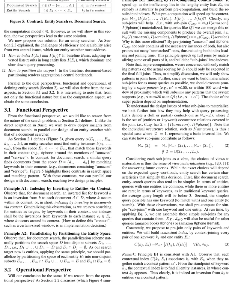
Baseline Implementation: In ourBasic approach, we index enti-ties the same way as we index keyword using the commonly used data structure: inverted index. A keyword inverted index records the occurrence table of the keywordI(kj)in an ordered list sorted by document id. Similarly for a specific entity typeEi, all its occur-rences can be stored in an inverted index, where entries are ordered by document id. This is the actual realization of occurrence rela-tionI(Ei)which we introduced in Section 2. To optimize and save space, all occurrences that appear in the same document can share
onedocid. 2 d 12d617 ... 6 d [23,p8,0.8] Ia=I(amazon): I#p=I(#phone): d9 ... 9 d 36 6 d 18 Is=I(service): 9 d 34 56 d 56 200 ] 9 . 0 , , 323 [ p10 ... 6 d [27,e81,1.0] I#e=I(#email): d99... 257d 5556 d645 68 d 56 97 d 45 75 d 56d 4797 ] 9 . 0 , , 45 [ p86 d97[50,p8,0.8]... 35 d ...
Figure 6: Inverted Index Example
Figure 6 shows the layout of the inverted listsIa,Is, andI#p for keywords “amazon”, “service”, and entities “#phone”,“#email” respectively. As we can see, the layout of an entity list resembles that of keywords, except that for each occurrence, instance id and confidence information are stored in addition to the position infor-mation.
The actual execution of entity search is essentially for each key-word and entity specified in the query, load their inverted lists into memory; advance all the lists in parallel checking intersecting doc-uments; for each document in the intersection of all lists, using the specified matching pattern to instantiate tuples and calculate their local scores; calculate the final score for each entity tuple by aggre-gating all its local scores.
Example 2 (AnsweringQ1using Inverted Index): Now let’s
ex-ecute queryQ1using the inverted index in Figure 6 with the Bina-rySum scoring function.
We will first load the three listsIa,Is,I#pandI#efrom disk and then advance these lists in parallel. We will find documentd6 is in the intersection of all the lists. Phone instancep8in this doc-ument is a matching tuple as the positions of keywords and entity (17, 18, 23 respectively) match the specified pattern. The Binary-Sum measure used will report local score 1 for this tuple. Notice instancep10in the document won’t be matched as it falls out of the window of size 20. Similarly, we will report the matching of instancep86with local score 1 in documentd9, andp8with local score 1 in documentd97.
Efficiency Problems: Although the whole matching process seems
to be straightforward, there are obvious redundant operations. First, many document entries that will not produce any matchings are loaded and checked (e.g., document entryd2in the “amazon” in-verted list, etc). Most of the document entries, noted using “...”, in the “#phohe” list do not need to be loaded. This could signif-icantly save index loading time. Moreover, document intersection check can also be avoided on such document entries. Second, many within-document pattern matching operations are also redundant as they will not produce any matchings (e.g., instancep10in document
d6).
Our Solution: These aspects motivate the need of pre-computation
to reduce unnecessary online computation, as we previously re-vealed in principle B1 in section 2.2. Our span model discussed in [7] restricts the pattern matching within a maximal window size of 100. Therefore, the super patternα∗in our implementation es-sentially requires to record all the joins between a keyword and an entity within window size 100.
6
d
Ca#p=C(amazon, #phone): [17,23,p8,0.8] 6
d
Cs#p=C(service, #phone): [18,23,p8,0.8] 6
d
Ca#e=C(amazon, #email): [17,27,p81,1.0] 6
d
Cs#e=C(service, #email): [18,27,p81,1.0] 9
d [34,45,p86,0.9]d97[45,50,p8,0.8] 9
d [36,45,p86,0.9]d97[45,50,p8,0.8]
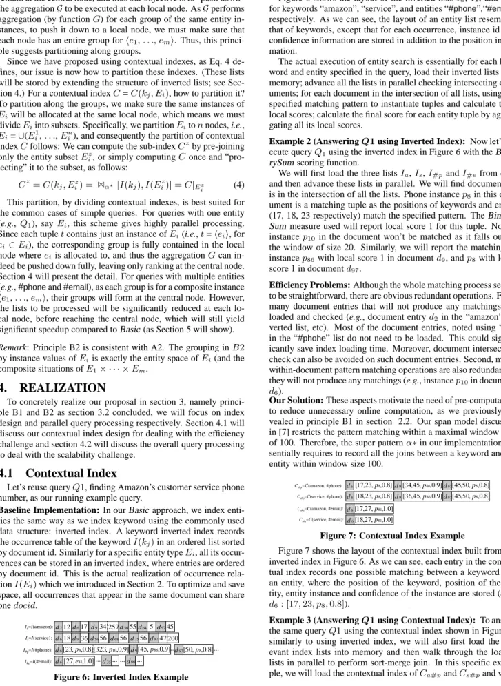
Figure 7: Contextual Index Example
Figure 7 shows the layout of the contextual index built from the inverted index in Figure 6. As we can see, each entry in the contex-tual index records one possible matching between a keyword and an entity, where the position of the keyword, position of the en-tity, entity instance and confidence of the instance are stored (e.g.,
d6: [17,23, p8,0.8]).
Example 3 (AnsweringQ1using Contextual Index): To answer
the same queryQ1using the contextual index shown in Figure 7, similarly to using inverted index, we will also first load the rel-evant index lists into memory and then walk through the loaded lists in parallel to perform sort-merge join. In this specific exam-ple, we will load the contextual index ofCa#pandCs#pand walk
through the two lists in parallel to find matchings. The exact same results will be produced. As we can see, the unnecessary loading and checking of entriesd2,d56,d64inIa, entriesd56,d68andd75 inIsand many entries inI#p(abbreviated by “...”) are voided. Fur-thermore, unnecessary matchings within documentd9and possible many more within other documents are also avoided.
contextual info docid entity conf entity inst entity pos keyword pos
...
...
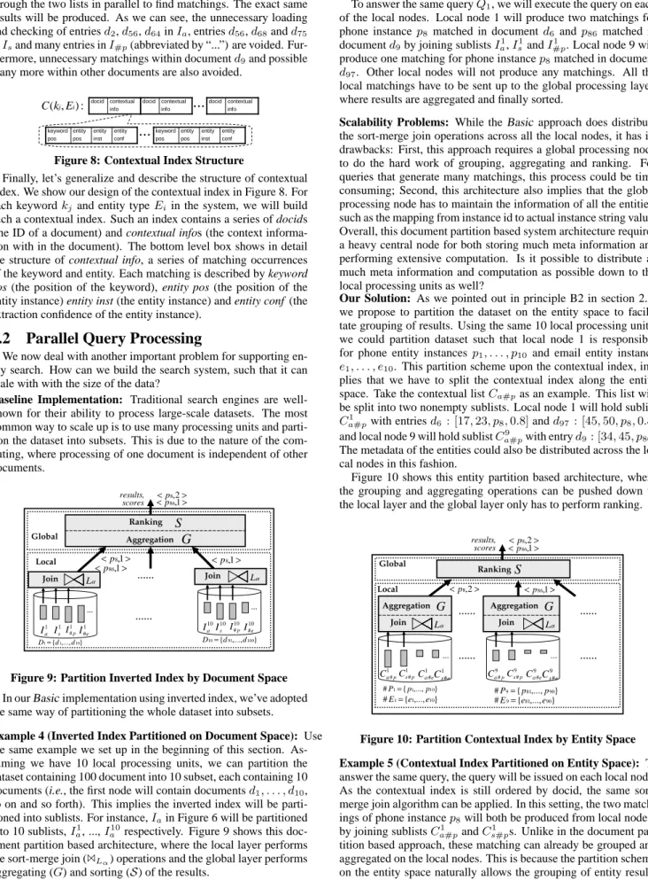
: ) , (kj Ei C contextual info docid contextual info docid entity conf entity inst entity pos keyword posFigure 8: Contextual Index Structure
Finally, let’s generalize and describe the structure of contextual index. We show our design of the contextual index in Figure 8. For each keywordkj and entity typeEiin the system, we will build such a contextual index. Such an index contains a series of docids (the ID of a document) and contextual infos (the context informa-tion with in the document). The bottom level box shows in detail the structure of contextual info, a series of matching occurrences of the keyword and entity. Each matching is described by keyword
pos (the position of the keyword), entity pos (the position of the
entity instance) entity inst (the entity instance) and entity conf (the extraction confidence of the entity instance).
4.2
Parallel Query Processing
We now deal with another important problem for supporting en-tity search. How can we build the search system, such that it can scale with with the size of the data?
Baseline Implementation: Traditional search engines are
well-known for their ability to process large-scale datasets. The most common way to scale up is to use many processing units and parti-tion the dataset into subsets. This is due to the nature of the com-puting, where processing of one document is independent of other documents. Join …… Aggregation Local Ranking } ,..., {1 10 1 d d D= D10={d91,...,d100} Global α L Join Lα
S
G
1 a I 1 s I 1 # p I 1 #e I … > <p8,1 > <p86,1 > <p8,1 > <p8,2 > <p86,1 results, scores …… 10 a I 10 s I 10 # p I 10 #e I …Figure 9: Partition Inverted Index by Document Space
In ourBasic implementation using inverted index, we’ve adopted the same way of partitioning the whole dataset into subsets.
Example 4 (Inverted Index Partitioned on Document Space): Use
the same example we set up in the beginning of this section. As-suming we have 10 local processing units, we can partition the dataset containing 100 document into 10 subset, each containing 10 documents (i.e., the first node will contain documentsd1, . . . , d10, so on and so forth). This implies the inverted index will be parti-tioned into sublists. For instance,Iain Figure 6 will be partitioned into 10 sublists,Ia1, ...,Ia10respectively. Figure 9 shows this doc-ument partition based architecture, where the local layer performs the sort-merge join (1Lα) operations and the global layer performs
aggregating (G) and sorting (S) of the results.
To answer the same queryQ1, we will execute the query on each of the local nodes. Local node 1 will produce two matchings for phone instance p8 matched in document d6 and p86 matched in documentd9by joining sublistsIa1,Is1andI#1p. Local node 9 will produce one matching for phone instancep8matched in document
d97. Other local nodes will not produce any matchings. All the local matchings have to be sent up to the global processing layer, where results are aggregated and finally sorted.
Scalability Problems: While theBasic approach does distribute the sort-merge join operations across all the local nodes, it has its drawbacks: First, this approach requires a global processing node to do the hard work of grouping, aggregating and ranking. For queries that generate many matchings, this process could be time consuming; Second, this architecture also implies that the global processing node has to maintain the information of all the entities, such as the mapping from instance id to actual instance string value. Overall, this document partition based system architecture requires a heavy central node for both storing much meta information and performing extensive computation. Is it possible to distribute as much meta information and computation as possible down to the local processing units as well?
Our Solution: As we pointed out in principle B2 in section 2.2,
we propose to partition the dataset on the entity space to facili-tate grouping of results. Using the same 10 local processing units, we could partition dataset such that local node 1 is responsible for phone entity instances p1, . . . , p10 and email entity instance
e1, . . . , e10. This partition scheme upon the contextual index,
im-plies that we have to split the contextual index along the entity space. Take the contextual listCa#pas an example. This list will be split into two nonempty sublists. Local node 1 will hold sublist
C1
a#pwith entriesd6 : [17,23, p8,0.8]andd97 : [45,50, p8,0.8] and local node 9 will hold sublistCa9#pwith entryd9: [34,45, p86,0.8]. The metadata of the entities could also be distributed across the lo-cal nodes in this fashion.
Figure 10 shows this entity partition based architecture, where the grouping and aggregating operations can be pushed down to the local layer and the global layer only has to perform ranking.
Join …… G Local Ranking Global
S
} ,..., { #E1= e1 e10 } ,..., { #P1= p1 p10 #P9={p81,...,p90} } ,..., { #E9= e81 e90 Aggregation α L Join G Aggregation α L 1 # p a C 1 # p s C 1 #e a C 1 #e s C … …… > <p8,2 > <p86,1 results, scores 9 # p a C 9 # p s C 9 #e a C 9 #e s C … > <p8,2 <p86,1> …… ……Figure 10: Partition Contextual Index by Entity Space Example 5 (Contextual Index Partitioned on Entity Space): To
answer the same query, the query will be issued on each local node. As the contextual index is still ordered by docid, the same sort-merge join algorithm can be applied. In this setting, the two match-ings of phone instancep8will both be produced from local node 1 by joining sublistsCa1#pandC1s#ps. Unlike in the document par-tition based approach, these matching can already be grouped and aggregated on the local nodes. This is because the partition scheme on the entity space naturally allows the grouping of entity results
possible on the local nodes. And once the matchings are grouped, their local scores can be aggregated to form the query score for each distinctive entity tuple. In this example, the final query score of phone instancep8is calculated on node 1 and that ofp86is cal-culated on node 9. Entity instances, along with their final scores, are send to the central processing unit, where the ranking is per-formed. As we can see, this design allows the possibility to move most of the computation on the central node down to the distributed local nodes.
As we have hinted in Section 3.2, this entity space partition scheme is based suited for entity search queries containing single entity type, which is the most basic and common entity query type. Now we discuss how to process query having multiple queries upon our contextual index partitioned on entity space scheme.
Let’s introduce an additional entity type#emailtoQ1, which gives us the following queryQ01: “ow20(amazon service#phone
#email)”. Figure 11 shows the overall framework for processing
Q0
1upon the contextual index partitioned on entity space.
Join …… Local Global 9 # p as C } ,..., { #E1= e1 e10 9 #e as C } ,..., { #P1= p1 p10 #P9={p81,...,p90} } ,..., { #E9=e81 e90 α Join 1 # p a C 1 # p s C 1 #e a C 1 #e s C … …… > <p8,e81,1 results, scores 9 # p a C 9 # p s C 9 #e a C 9 #e s C … …… …… α 1 #e as C 1 # p as C Aggregation Ranking S G
Merge & Join Lα
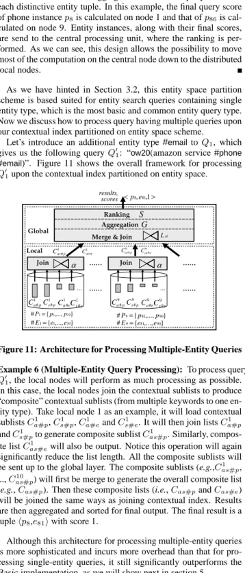
Figure 11: Architecture for Processing Multiple-Entity Queries Example 6 (Multiple-Entity Query Processing): To process query Q0
1, the local nodes will perform as much processing as possible. In this case, the local nodes join the contextual sublists to produce “composite” contextual sublists (from multiple keywords to one en-tity type). Take local node 1 as an example, it will load contextual sublistsC1
a#p,Cs1#p,Ca1#eandCs1#e. It will then join listsCa1#p andCs1#pto generate composite sublistC1as#p. Similarly, compos-ite listC1
as#ewill also be output. Notice this operation will again significantly reduce the list length. All the composite sublists will be sent up to the global layer. The composite sublists (e.g.,C1
as#p, ...,C10
as#p) will first be merge to generate the overall composite list (e.g.,Cas#p). Then these composite lists (i.e.,Cas#pandCas#e) will be joined the same ways as joining contextual index. Results are then aggregated and sorted for final output. The final result is a tuplehp8,e81iwith score 1.
Although this architecture for processing multiple-entity queries is more sophisticated and incurs more overhead than that for pro-cessing single-entity queries, it still significantly outperforms the Basic implementation, as we will show next in section 5.
5.
EXPERIMENTS
In order to empirically study the effectiveness of our novel index design, contextual index, and parallel query processing framework for supporting efficient entity search, we have build a large-scale, distributed system using theYellowPage scenario on a real Web corpus. In this section, we will first briefly discuss the setup of our system. Then, we will use three benchmark query sets to show
that by leveraging contextual indexing and joining, we can speed up query processing by orders of magnitude.
5.1
Experiment Setup
To empirically verify that indexing and query processing design is effective for supporting efficient entity search, we decide to use the Web, the ultimate information source, as our corpus. Our cor-pus, a general Web crawl in Aug, 2006, is obtained from the Web-Base Project. The total size is around 2TB, containing 48974 web-sites and 93 million pages.
To process such terabyte-sized data set, we ran our indexing and query processing modules on a cluster of 34 machines, each with dual 500 Mhz Pentium III CPU, 1 GB memory and 160 GB of disk. 33 out of the 34 nodes are used as local indexing and processing units, whereas 1 node is used as the central aggregation node.
On this corpus, we target at two entity types: phone and email. They are extracted based on a set of regular expression rules. We extracted around 8,800,432 distinctive phone entity instances and 4,646,009 distinctive email entity instances.
We implemented both theBasicinverted index based approach and the contextual index based approach. In the inverted index based approach, we evenly distribute the whole corpus across the 33 local nodes by partitioning based on document IDs. In the con-textual index based approach, we partition the concon-textual index on entity IDs. Each local node will be responsible for the same number of distinct entity instances for each entity type. For instance, email entity instances with ID in the range of 1 - 140,778 and phone en-tity instances with ID in the range of 1 - 266,680 will be indexed and only indexed on the first local node.
5.2
Experiment Results
To study the performance of our method in a systematical way, we use the following three benchmark query sets for evaluation.
Benchmark I (phone related): We use the names of top 30
com-panies in Fortune 500, 2006 as part of our query, together with phone entity type in the query. Benchmark II (email related): We use the names of 88 PC members of SIGMOD 2007 as part of our query, together with email entity type in the query. Benchmark III
(email & phone related): We use the names of 88 PC members of
SIGMOD 2007 as part of our query, together with email entity type and phone entity type in the query.
The reason why we select those three benchmark query sets are the following: First, those three benchmark query sets contains both simple single-entity queries (Benchmark I&II) and complex multiple-entity queries(Benchmark III). Second, the selectivity of the keywords also differs quite a lot. Keywords used in Benchmark I query set (e.g.“Walmart”, ”Chevron”, etc) are far less selective than the ones used in benchmark II&III query sets (e.g.“Ailamaki”, “Chakrabarti”, etc). Third, the number of keywords in those three query sets also has good variation, in the range from one keyword to three keywords. Finally, all the queries used in those bench-mark query sets are real queries and useful in practise. Overall, we believe those three benchmark query sets are typical and represen-tative for a wide range of entity search queries.
To measure query processing on local processing units, where most of the computation are done, we look at the following four as-pects for processing each query: List length - the size of index lists that is needed to load for processing query; Index loading time - the time needed to load index into disk; Joining time - the time needed to join the loaded index lists for producing entity tuples; Processing time - the time needed to load and join index for query processing. For each aspect, we measure the overall statistics summed over all the local processing units and the max statistic of all the local pro-cessing units. Take the propro-cessing time as an example, we measure both the sum of the processing time spent on all local processing units as well as the max processing time among all the local
pro-cessing units. The overall propro-cessing time indicates the throughput of the system, whereas the max processing time indicates the query response time of the system. Throughput and query response time are all primary measures for measuring search engines.
We define the selectivity of a query as the overall list length reduction using contextual index versus inverted index. The higher the reduction, the higher the selectivity.
To get robust experimental results, we execute each query 10 times. To eliminate the effect of cold start, the results from the first two runs are discarded. The results from the remaining eight runs are averaged and used for experimental study.
0 5 10 15 20 25 30 10−1 100 101 102 103 104 105 106 Query Number
List Length Reduction (Times)
Overall Max
(a) List Length Comparison
0 5 10 15 20 25 30 10−1 100 101 102 103 104 Query Number
Loading Index Speedup (Times)
Overall Max
(b) Index Loading Time Compari-son 0 5 10 15 20 25 30 100 101 102 103 104 Query Number
Joining Speedup (Times)
Overall Max
(c) Join Time Comparison
0 5 10 15 20 25 30 100 101 102 103 104 Query Number
Query Processing Speedup (Times)
Overall Max
(d) Processing Time Comparison
Figure 12: Benchmark I (Phone Related)
Experiment results on query efficiency for the three benchmark query sets are shown in Figures 12, 13, 14 respectively. Now let’s zoom into Figure 12 and reveal details of the results.
Figure 12(a) shows the index list length reduction in log scale for each query. The queries are ordered in ascending order according to their selectivity. The queries in Figures 12(b), 12(c) and 12(d) are ordered according to their order in Figure 12(a). Figure 12(b) shows the index loading speedup in log scale for each query. Fig-ure 12(c) shows the index joining speedup in log scale for each query. Figure 12(d) shows the query processing speedup in log scale for each query. As we can see, there are strong correlations between the query selectivity and index loading time, joining time and processing time respectively. Figures 13 and 14 show similar result patterns for Benchmark II&III.
As we can see, most of the queries can be speedup by at least two orders of magnitude. We do observe less speedup in Bench-mark II&II than BenchBench-mark I. We believe this is mainly due to the difference in selectivity as the keywords used in Benchmark I are far less selective. Consequently, the saving in reducing list length as well as joining is not as much. We also observe the loading and processing speedup clearly flattens for queries that have high re-duction in list length (where the contextual index are normally very short). This is because index loading consisting of random seek time and sequential read time. For queries that have short contex-tual lists, the random seek time plays a significant role.
In Figure 15(a), we report the query processing speedup with re-gard to the number of keywords in a query. To keep the number of
0 10 20 30 40 50 60 70 80 90 100 101 102 103 104 105 Query Number
List Length Reduction (Times)
Overall Max
(a) List Length Comparison
0 10 20 30 40 50 60 70 80 90 100 101 102 103 104 Query Number
Loading Index Speedup (Times)
Overall Max
(b) Index Loading Time Compari-son 0 10 20 30 40 50 60 70 80 90 100 101 102 103 104 Query Number
Joining Speedup (Times)
Overall Max
(c) Join Time Comparison
0 10 20 30 40 50 60 70 80 90 100 101 102 103 104 Query Number
Query Processing Speedup (Times)
Overall Max
(d) Processing Time Comparison
Figure 13: Benchmark II (Email Related)
0 10 20 30 40 50 60 70 80 90 10−1 100 101 102 103 104 105 Query Number
List Length Reduction (Times)
Overall Max
(a) List Length Comparison
0 10 20 30 40 50 60 70 80 90 100 101 102 103 104 105 Query Number
Loading Index Speedup (Times)
Overall Max
(b) Index Loading Time Compari-son 0 10 20 30 40 50 60 70 80 90 101 102 103 104 105 Query Number
Joining Speedup (Times)
Overall Max
(c) Join Time Comparison
0 10 20 30 40 50 60 70 80 90 101 102 103 104 105 Query Number
Query Processing Speedup (Times)
Overall Max
(d) Processing Time Comparison
Figure 14: Benchmark III (Email & Phone Related)
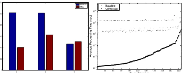
entities a constant across all queries, we use all queries from Bench-mark I and II. The number of keywords varies from one to three in the queries in Benchmark I and II. As we can see in Figure 15(a), all three query classes has speedup for more than two orders of magnitude on average regardless of the number of keywords. In Figure 15(b), we report the average query processing time com-parison for all queries in Benchmark I, II and III. The queries are ordered in ascending order according to their average processing time using the contextual index approach. As we can see, contex-tual index based approach achieves two orders of magnitude over
1 2 3 0 100 200 300 400 500 600 Number of Keywords
Query Processing Speedup (Times)
Overall Max
(a) Speedup w.r.t. Number of Keywords 20 40 60 80 100 120 140 160 180 200 10−3 10−2 10−1 100 101 102 Query Number
Average Processing Time (sec)
Baseline Contextual
(b) Average Processing Time Comparison
Figure 15: Comparison across Different Benchmarks
the baseline approach for most queries.
In addition to experiment the local query processing speedup, we’ve also tested the network transfer cost between the local layer and the global layer, as well as the processing cost that occurs on the global layer. While we observe the contextual based approach generally requires much less network transfer cost as well as global processing cost, the costs are insignificant comparing to the local query processing costs and are therefore omitted for detailed dis-cussion.
In terms of index size, our contextual index only is roughly 1/6 of the size of the inverted index. However, we need to point out that the index size is highly related with the number of entity types supported in the system. While in thisYellowPage scenario, email and phone entity type are the only interesting entity types we con-sider, other application could support more entities types. In such cases, there is a chance that the contextual index size will overtake the inverted index size. However, we believe contextual index is still worth to utilize as nowadays disks are becoming cheaper while query processing is always in need for optimization.
6.
RELATED WORK
We formulate the problem of entity search and emphasize its ap-plication on information integration in [6]. Our prototype search system is revealed in [8]. We study one of the core challenges for supporting entity search - the entity ranking problem - in [7]. We are now witnessing an emerging research trend on using entities and relationships to facilitate various search and mining tasks [4, 5, 17, 15, 13, 12, 1, 2, 3, 14, 19]. We have discussed the relation-ship between our work and these works in detail in the related work section of [7].
Our work is most related with the works on indexing unstruc-tured documents. Inverted index [21] has been widely used in search engines for answering keywords queries. Although it is gen-eral and can support many different query types, it is not optimized for queries such as phrase queries, proximity based queries, etc. Cho [9] builds a multigram index over a corpus to support fast reg-ular expression matching. A multigram index is essentially build-ing a postbuild-ing list for selective multigrams. It can help to narrow down the matching scope. Again, it is not optimized for phrase or proximity queries and still require full scan of candidate doc-uments. Nextword index [18] is a structure designed to speed up phrase queries and to enable some amount of phrase browsing. It is an inverted index where each term list contains a list of the suc-cessor words found in the corpus. Each sucsuc-cessor word is followed by position information. This index is optimized for answering keyword phrase queries. It doesn’t consider more flexible proxim-ity based queries and doesn’t consider types other than keywords. BE [1] develops a search engine based on linguistic phrase patterns and utilizes a special “neighborhood index” for efficient process-ing. Although BE considers indexing types such as noun phrases
other than keywords, its index is limited to phrase queries only. Chakrabarti et al. [5] introduce a class of text proximity queries and study scoring function and index structure optimization for such queries. Their study on index is more on reducing the redundancy, rather than improving efficiency. A recent work [10] studies the indexing problem on dataspace. While this work also tries to ex-ploit the relationship between keyword and structure, its angle from dataspace is very different from that of ours. Therefore, its index design is also very different from our contextual index.
7.
CONCLUSIONS
In this paper, we develop query indexing and processing for mak-ing entity search efficient and scalable. From the functional defi-nition of entity search, we derive the operational defidefi-nition, from both of which we derive our proposal. Unlike the natural base-line of indexing entities as keywords, we develop contextual joins, which materializes pre-joins between entities and keywords. We further develop data parallelization by entity-space partitioning, un-like the traditional document-space partition approach. Our exper-iments show significant 200-500 times of speedup and sub-second response time.
8.
REFERENCES
[1] M. Cafarella and O. Etzioni. A search engine for large-corpus language applications. In WWW, 2005.
[2] M. Cafarella, C. Re, D. Suciu, and O. Etzioni. Structured querying of web text data: A technical challenge. In CIDR, 2007.
[3] K. Chakrabarti, V. Ganti, J. Han, and D. Xin. Ranking objects based on relationships. In SIGMOD, 2006.
[4] S. Chakrabarti. Breaking through the syntax barrier: Searching with entities and relations. In ECML, pages 9–16, 2004.
[5] S. Chakrabarti, K. Puniyani, and S. Das. Optimizing scoring functions and indexes for proximity search in type-annotated corpora. In WWW, pages 717–726, 2006.
[6] T. Cheng and K. C.-C. Chang. Entity search engine: Towards agile best-effort information integration over the web. In CIDR, pages 108–113, 2007.
[7] T. Cheng and K. C.-C. Chang. Entityrank: Searching entities directly and holistically. In VLDB, 2007.
[8] T. Cheng, X. Yan, and K. C.-C. Chang. Supporting entity search: A large-scale prototype search system. In SIGMOD, 2007.
[9] J. Cho and S. Rajagopalan. A fast regular expression indexing engine. In ICDE, 2002.
[10] X. Dong and A. Halevy. Indexing dataspaces. In SIGMOD, 2007. [11] H. Gupta. Selection of views to materialize in a data warehouse. In
ICDT, pages 98–112, 1997.
[12] E. Kandogan, R. Krishnamurthy, S. Raghavan, S. Vaithyanathan, and H. Zhu. Avatar semantic search: a database approach to information retrieval. In SIGMOD, pages 790–792, 2006.
[13] G. Kasneci, F. M. Suchanek, M. Ramanath, and G. Weikum. How naga uncoils: searching with entities and relations. In WWW, 2007. [14] Z. Nie, Y. Ma, S. Shi, J.-R. Wen, and W.-Y. Ma. Web object retrieval.
In WWW, 2007.
[15] J. Stoyanovich, S. Bedathur, K. Berberich, and G. Weikum. Entityauthority: Semantically enriched graph-based authority propagation. In WebDB, 2007.
[16] J. D. Ullman and J. Widom. A First Course in Database Systems. Prentice-Hall, 1997.
[17] G. Weikum. Db&ir: both sides now. In SIGMOD, 2007. [18] H. E. Williams, J. Zobel, and D. Bahle. Fast phrase querying with
combined indexes. ACM Trans. Inf. Syst., 22(4):573–594, 2004. [19] M. Wu and A. Marian. Corroborating answers from multiple web
sources. In WebDB, 2007.
[20] J. Yang, K. Karlapalem, and Q. Li. Algorithms for materialized view design in data warehousing environment. In The VLDB Journal, pages 136–145, 1997.
[21] J. Zobel and A. Moffat. Inverted files for text search engines. ACM