Heterogeneous Medical Data Processing

(1)

University of West Bohemia

Department of Computer Science and Engineering Univerzitni 8

30614 Pilsen Czech Republic

Heterogeneous Medical Data

Processing

PhD Study Report

Ing. Tomáš Prokop

Technical Report No. DCSE/TR-2017-01 May, 2017

(2)

Technical Report No. DCSE/TR-2017-01 May 2017

Heterogeneous

Medical

Data

Processing

Tomáš Prokop

Abstract

Electroencephalography (EEG) is a popular technique used for example in diagnostics of diseases, sleep monitoring and neurorehabilitations. Due to increasing mobility and decreasing price of EEG measuring devices EEG and ERP (event related potential) techniques have become more widespread also in assistive technologies and brain-jogging. As the result the amount of EEG data has been increasing and research into EEG signal processing and classification has become again more necessary.

This thesis focuses on the state-of-the-art related to the methods of EEG/ERP signal processing and classification, but follows a standard processing workflow starting from signal acquisition and preprocessing to feature extraction and classification. The commonly used time-frequency domain methods (Wavelet transform and Matching pursuit) that are suitable for feature extraction are described together with the Hilbert-Huang Transform (HHT). HHT uses a new approach of multi-channel signal decomposition called the Multivariate Empirical Mode Decomposition.

The described classification methods are divided into two groups. Linear classifiers are represented by the Linear Discriminant Analysis and Support Vector Machines. The second group, neural networks, focuses on the Multi-Layer Perceptron and a set of classification algorithms called deep learning neural networks. These are composed of many layers of neurons while the Multi-Layer Perceptron typically contained only two layers because of the backpropagation problem. Some of the deep learning algorithms have been reported to beat state-of-the-art approaches in many applications and that is why further research in the EEG domain seems to be beneficial.

This work was supported by identification of grant or project.

Copies of this report are available on

http://www.kiv.zcu.cz/publications/

or by surface mail on request sent to the following address: University of West Bohemia in Pilsen

Department of Computer Science and Engineering Univerzitni 8

30614 Pilsen Czech Republic

(3)

1. Introduction

The development of assistive technologies for people with physical limitations has become a new world trend in recent years. Assistive technologies are used to monitor people, to help them communicate with outer world, to assist with their movement and to control devices. Assistive systems that enable people to control computers or other devices are based on brain-computer interfaces, gestures, eye blinking (EOG), muscle contraction (EMG) or other signals depending on health condition of the user. Seniors or injured people are mostly the target group.

Electroencephalography (EEG) is a very popular technique not only for diagnostics of diseases, sleep monitoring or neurorehabilitations, but also for so called brain-jogging or assistive systems. The use of the human brain to control specific devices or applications is called brain-computer interface (BCI). BCI assistive technologies use EEG or event related potentials (ERP), which are often combined with other bio signals (e.g. EOG or EMG) to improve stability and performance of the system.

The amount of measured EEG data increases every year. The main reasons are new application areas of EEG and newly developed EEG equipment, which is available to public because of its price and usability. With the increasing amount of EEG data the need for automatic analysis, classification and interpretation is also rising. Classification and interpretation of EEG data is a complex problem and it is difficult to understand EEG data even for experts. Automatic EEG data processing is also necessary for BCI based assistive systems. These reasons lead to the development of new methods and improvement of existing methods for EEG/ERP data processing and classification.

The main aim of this thesis is to provide introduction into processing and classification methods suitable for BCI systems that are based on EEG/ERP. Most of the described methods are widely used in the EEG/ERP technique but they are also suitable for the processing of other heterogeneous bio signals. The second goal is to define the aims of the Ph.D. thesis.

One of relatively new and unexplored approaches in the EEG/ERP classification is the use of deep learning algorithms that seems to be very promising due to good results in the domain of natural language processing and image processing.

The Introduction section is followed by the description of the origin of the electroencephalographic signal, its properties and content of EEG signal records. The third chapter is dedicated to event-related potentials. The next section contains the description of the methods usually used to preprocess the EEG and ERP signal. Section 5 describes widely used time-frequency domain algorithms for ERP waveform detection and feature extraction. Linear classifiers and neural networks are explored in the following section. The end of this document belongs to the conclusion and aims of the Ph.D. thesis.

(6)

Page 2

2. Electroencephalography

Electroencephalography (EEG) is a diagnostic method used for measuring electrical activity of the brain. The measuring device is called electroencephalograph and the record of the electrical activity measured by electroencephalograph is electroencephalogram. EEG signal is a time variation of potential diﬀerence between two electrodes placed on the patient’s scalp surface.

2.1. Origin of EEG Signal

The basic functional unit of the nervous system is the nerve cell - the neuron - which communicates information to and from the brain. Neurons can be classified with reference to morphology or functionality. Three basic types of neurons can be defined: sensory neurons, connected to sensory receptors, motor neurons, connected to muscles, and interneurons, connected to other neurons. [1]

The archetypal neuron consists of a cell body, the soma, from which two types of structures extend: the dendrites and the axon, see Figure 2.1. Dendrites can consist of as many as several thousands of branches, with each branch receiving a signal from another neuron. The axon is usually a single branch which transmits the output signal of the neuron to various parts of the nervous system. The transmission of information from one neuron to another takes place at the synapse, a junction where the terminal part of the axon contacts another neuron. The signal, initiated in the soma, propagates through the axon encoded as a short, pulse-shaped waveform, i.e., the action potential. Although this signal is initially electrical, it is converted in the presynaptic neuron to a chemical signal (“neurotransmitter”) which diffuses across the synaptic gap and is subsequently reconverted to an electrical signal in the postsynaptic neuron, see Figure 2.1(b). [1]

An EEG signal is a measurement of currents that flow during synaptic excitations of the dendrites of many pyramidal neurons in the cerebral cortex. When neurons are activated, the synaptic currents are produced within the dendrites. This current generates a magnetic field measurable by electromyogram (EMG) machines and a secondary electrical field over the scalp measurable by EEG systems. [2]

The human head consists of different layers including the scalp, skull, brain, and many other thin layers in between. The skull attenuates the signals approximately one hundred times more than the soft tissue. On the other hand, most of the noise is generated either within the brain (internal noise) or over the scalp (system noise or external noise). Therefore, only large populations of active neurons can generate enough potential to be recordable using the scalp electrodes. These signals are later amplified greatly for display purposes. [2]

(7)

Figure 2.1: (a) An archetypal neuron and (b) three interconnected neurons. A presynaptic neuron transmits the signal toward a synapse, whereas a postsynaptic neuron transmits the signal away from the synapse. [1]

2.2. Basic EEG Rhythms

Basic EEG rhythms are listed below. Alpha, Beta, Delta and Theta rhythms are visible in Figure 2.2.

 Delta rhythm lies within the frequency range from 0.5 Hz to 4 Hz and has amplitude usually higher than 10 μV. Delta waves are primarily associated with deep sleep and may be present in the waking state. [2]

 Theta waves are in the frequency range of 4 – 7.5 Hz. Theta waves appear as consciousness slips towards drowsiness. Theta waves have been associated with access to unconscious material, creative inspiration and deep meditation. [2]

 Alpha waves have frequency from 8 to 13Hz and amplitude between 30 μV and 50 μV. Alpha waves have been thought to indicate both a relaxed awareness without any attention or concentration. The alpha wave is the most prominent rhythm in the whole realm of brain activity and possibly covers a greater frequency range than has been previously accepted. [2]

 Beta rhythm frequency varies from 14 Hz to 30 Hz and its amplitude lies within range from 5 μV to 30 μV. A beta wave is the usual waking rhythm of the brain associated with active thinking, active attention, focus on the outside world, or solving concrete problems, and is found in normal adults. [2]

 Gama rhythm frequency is usually higher than 30Hz. The amplitudes of these rhythms are very low and their occurrence is rare. The gamma wave band has

(8)

Page 4 been proved to be a good indication of event-related synchronization (ERS) of the brain and can be used to demonstrate the locus for right and left index ﬁnger movement, right toes, and the rather broad and bilateral area for tongue movement [3].[2]

Figure 2.2: Four typical dominant brain normal rhythms, from high to low frequencies.[2]

2.3. EEG signal Recording

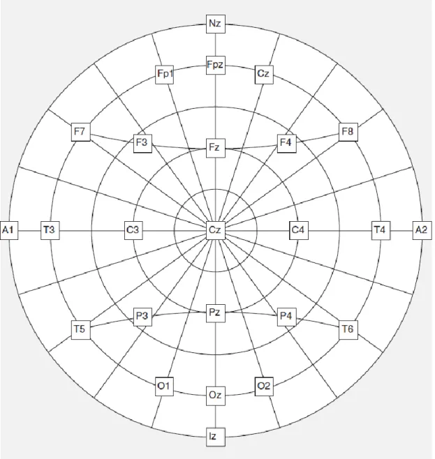
For multichannel recordings with a large number of electrodes, electrode caps are often used. The International standard for electrode placement is called 10–20 system. It consists of 21 electrodes (excluding the earlobe electrodes). Often the earlobe electrodes called A1 and A2, connected respectively to the left and right earlobes, are used as the reference electrodes. The 10–20 system avoids both eyeball placement and considers some constant distances by using specific anatomic landmarks from which the measurement would be made and then uses 10 or 20% of that specified distance as the electrode interval. The odd electrodes are on the left and the even ones on the right. [2]

Additional electrodes can be used to acquire EOG, EMG or ECG signal. This is useful for artifact detection or reduction as is mentioned in Section 2.4. The number of electrodes used and electrode placement depend on the origin of an ERP waveform and experimental design. Even single channel recording may be used e.g. in brain-computer interfaces [2]. On the other hand, more than 64 electrodes should be used in the brain mapping applications.

(9)

Figure 2.3: A conventional 10/20 system with 21 electrodes. A1 and A2 earlobe electrodes are used as the reference electrodes. [4]

A raw EEG signal has amplitudes of the order of μV and contain frequency components of up to 300 Hz. To retain the effective information the signal has to be amplified before it is digitalized by the analogue-digital converter (ADC) and filtered, either before or after the ADC, to reduce the noise and make the signals suitable for processing and visualization. The commonly used sampling frequencies for EEG recordings are 100 Hz, 250 Hz, 500 Hz, 1000 Hz, and 2000 Hz. [2]

The main application areas of the EEG technique are:

 Epilepsy - EEG is the principal test for diagnosing epilepsy and gathering information about the type and location of seizures.

(10)

Page 6

 Sleep Disorders – Diagnosis of sleep disorders like Insomnia, Hypersomnia, Parasomnia or Circadian rhythm disorder is provided.

 Brain-computer interfaces - A brain-computer interface (BCI) enables a subject to communicate with and control the external world without using the brain's normal output through peripheral nerves and muscles [5-7]. Messages are conveyed by spontaneous or evoked EEG activity rather than by muscle contractions. [1]

2.4. Artifacts

One of the crucial aspects in biomedical signal processing is to acquire knowledge about noise and artifacts which are present in the signal so that their influence can be minimized. A useful categorization of artifacts is based on their origin, i. e., those of physiological or technical origin. While the influence of artifacts of technical origin can be reduced to a large degree by paying extra attention to the attachment of electrodes to the body surface, it is impossible to avoid the influence of artifacts of physiological origin. Accordingly, majority of algorithms developed for EEG artifact processing are intended for the reduction of physiological artifacts. [1]

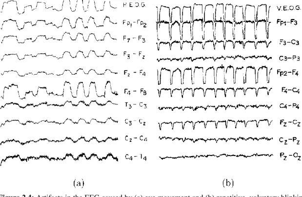
Figure 2.4: Artifacts in the EEG caused by (a) eye movement and (b) repetitive, voluntary blinking.

The signal at the top of each column shows the horizontal and vertical EOG, respectively. [8]

2.4.1. Biological Artifacts

Eye movements and blinks: Eye movement produces electrical activity (EOG) which is strong enough to be clearly visible in EEG. EOG reflects the potential difference between the cornea and retina which changes during eye movement. The measured voltage is almost proportional to the angle of gaze [9]. The strength of the EOG signal depends on the distance of the electrode to the eye and the direction in which the eye is

(11)

moving. The waveforms produced by repeated eye movement are exemplified in Figure 2.4(a). [1]

Another common artifact is caused by eyelid movement ("blinks”). The blinking artifact usually produces a more abruptly changing waveform than eye movement, and, accordingly, the blinking artifact contains more high-frequency components. This particular signal characteristic is exemplified in Figure 2.4(b).

From an artifact processing viewpoint, it is highly practical if a "pure" EOG signal can be acquired by means of two reference electrodes positioned near the eye which do not contain any EEG activity. [1]

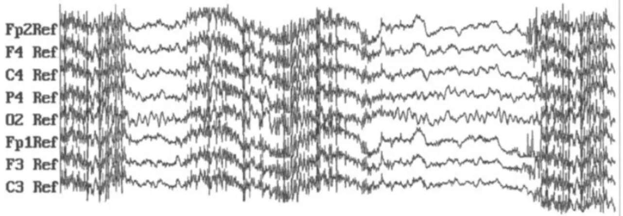
Muscle Activity: Contracting muscles cause electrical activity that can be present in the EEG signal, see Figure 2.5. Activity is measured on the body surface by the Electromyogram (EMG). This type of artifact is primarily encountered when the patient is awake and occurs during swallowing, grimacing, frowning, chewing, talking, sucking, and hiccupping [8]. The muscle artifact is considerably reduced during relaxation and sleep. [1]

Figure 2.5: A 5-s, multichannel EEG recording contaminated with intermittent episodes of EMG

artifacts. [10]

Cardiac Activity: The electrical activity of the heart, as reflected by ECG, can interfere with EEG. Although the amplitude of the cardiac activity is usually low on the scalp in comparison to the EEG amplitude (1-2 and 20-100 μV, respectively), it can hamper the EEG considerably at certain electrode positions and for certain body shapes [11]. The repetitive, regularly occurring waveform pattern which characterizes the normal heartbeats fortunately helps to reveal the presence of this artifact.

Similar to the eye-related artifacts mentioned above, the ECG can be acquired independently by one or several electrodes for use in canceling the ECG activity that may be superimposed on EEG. [1]

2.4.2. Technical Artifacts

Movement of electrodes causes changes in the DC contact potential at the electrode-skin interface which produces an artifact commonly referred to as the "electrode-pop" artifact. This type of technical artifact is not unique to the EEG signal, but may occur in any bioelectric signal measured on the body surface [12, 13]. The electrode- pop artifact is usually manifested as an abrupt change in the baseline level, followed by a slow, gradual return to the original baseline level. The electrode wire which connects the

(12)

Page 8 electrode to the acquisition equipment is another possible source of artifact. Insufficient shielding of the electrode wire makes it susceptible to electromagnetic fields caused by currents flowing in nearby powerlines or electrical devices. As a result, 50/60 Hz powerline interference is picked up by the electrodes and contaminates the EEG signal. Finally, equipment-related artifacts include those produced by internal amplifier noise and amplitude clipping caused by an analog-to-digital converter with too narrow dynamic range. [1]

(13)

3. Event-related Potentials

An event-related potential (ERP) is the measured response of the brain to a specific sensory, cognitive, or motor event (stimulus). More formally, it is any stereotyped electrophysiological response to a stimulus. [4]

3.1. Naming Convention

ERP waveforms consist of a sequence of positive and negative voltage deflections, which are called peaks, waves or components [4]. Name of most components starts with a letter P for positive amplitude peaks, N for negative amplitude peaks or C for components which have not dedicated one polarity. The letter is followed by a number indicating either the position within a waveform or a latency of the peak. For example, the third positive component can be referred as P3 or by its latency as P300.

3.2. Major ERP Components

An averaged ERP waveform that consists of P1, N1, P2, N2 and P3 components is visible in Figure 3.1.

3.2.1. Visual sensory responses

C1: The first major visual ERP component is usually called the C1 wave. It is not labeled with a P or an N because its polarity can vary. The C1 wave typically onsets 40– 60 ms poststimulus and peaks 80–100 ms poststimulus, and it is highly sensitive to stimulus parameters, such as contrast and spatial frequency. [4]

P1: The C1 wave is followed by the P1 wave, which is largest at lateral occipital electrode sites and typically onsets 60–90 ms poststimulus with a peak between 100– 130ms. The P1 onset time is difficult to assess accurately due to overlap with the C1 wave. In addition, P1 latency will vary substantially depending on stimulus contrast. [4] N1: The P1 wave is followed by the N1 wave. There are several visual N1 subcomponents. The earliest subcomponent peaks 100 – 150 ms poststimulus at anterior electrode sites, and there appear to be at least two posterior N1 components that typically peak 150 – 200 ms poststimulus, one arising from parietal cortex and another arising from lateral occipital cortex. [4]

P2: A distinct P2 wave follows the N1 wave. This component is larger for stimuli containing target features, and this effect is enhanced when the targets are relatively infrequent. In this sense, the anterior P2 wave is similar to the P3 wave. The P2 wave is often difficult to distinguish from the overlapping N1, N2, and P3 waves. [4]

3.2.2. Auditory sensory responses

N1: Like the visual N1 wave, the auditory N1 wave has several distinct Subcomponents. A frontocentral component that peaks around 75 ms, a vertex-maximum potential of unknown origin that peaks around 100 ms, and a more laterally distributed component that peaks around 150 ms. The N1 wave is sensitive to attention.

(14)

Page 10

Mismatch Negativity: The mismatch negativity (MMN) is observed when subjects are exposed to a repetitive train of identical stimuli with occasional mismatching stimuli. The mismatching stimuli elicit a negative-going wave that is largest at central midline scalp sites and typically peaks between 160 and 220 ms. [4]

The N2 family: Researchers have identified many clearly different components in N2 time range. A repetitive, nontarget stimulus will elicit an N2 deflection that can be thought of as the basic N2. If other stimuli are occasionally presented within a repetitive train, larger amplitude is observed in the N2 latency range. If these stimuli are irrelevant tones, this effect will consist of mismatch negativity. If the stimuli are task-relevant, then a somewhat later N2 effect is also observed, called N2b (the mismatch negativity is sometimes called N2a). This component is larger for less frequent targets, and it is thought to be a sign of the stimulus categorization process. Both auditory and visual stimuli will, if task-relevant, elicit an N2b component. [4]

The P3 family: There are several distinguishable ERP components in the time range of the P3 wave. Two main components are P3a and P3b. Both are elicited by unpredictable, infrequent shifts in tone pitch or intensity, but the P3b component is present only when these shifts are task-relevant. When ERP researchers refer to the P3 component or the P300 component, they almost always mean the P3b component. [4]

(15)

Figure 3.1: Averaged ERP waveform of non-target stimulus (Xs) and target stimulus (Os). P1, N1, P2, N2 and P3 components are clearly visible. [4]

(16)

Page 12

4. ERP Data Preprocessing

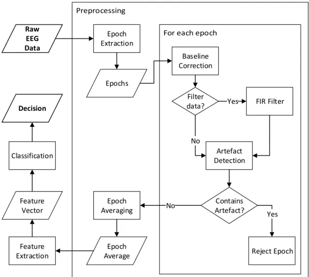
One of the possible ERP data processing workflows can be seen in Figure 4.1. Raw EEG data are first preprocessed using the following procedure: epoch extraction, baseline correction, filtering, artifact rejection or artifact cancelation, and epoch averaging. Preprocessing steps may differ depending on experimental design, e.g. raw EEG signal can be first filtered or filter can be applied later for each epoch. The epoch averaging is not present in the case of single-trial ERP waveform detection. Preprocessing is followed by feature extraction and subsequent classification.

Raw EEG Data Epoch Extraction Baseline Correction FIR Filter Feature Extraction No Filter data? Yes Classification Feature Vector Artefact Detection Contains Artefact? Epoch Averaging No _Yes Reject Epoch Epochs Epoch Average Decision

Figure 4.1: ERP data processing workflow. Some steps may differ depending on the experimental

design.

4.1. Epoch Extraction

Epoch extraction is an essential procedure in ERP data processing. An epoch is a segment of EEG signal around a stimulus. It is typically defined by the number of milliseconds before and after the stimulus. The prestimulus interval is highly important for the baseline correction described in the next section. The length of the poststimulus interval depends on properties of the processed ERP component and on the setup of the

(17)

experiment. The output of the epoch extraction method is a list of epochs. All extracted epochs acquired in one experiment must have the same length.

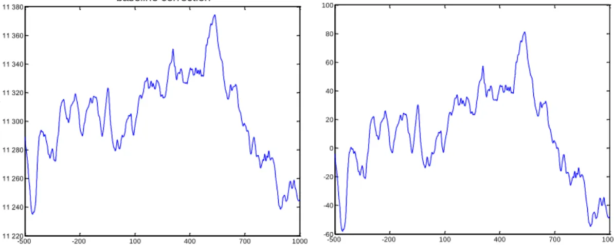
4.2. Baseline Correction

Impedance of the electrodes may vary every trial. There are mainly two reasons that cause this problem – drying of the conductive gel or sweating of the measured subject. The problem becomes bigger when we compute average from the epochs with different levels of baseline. The amplitude of the averaged ERP waveform depends on the values of baseline instead of amplitudes of the ERP waves.

This problem can be handled by a baseline correction method. It is a simple method that first computes average of first N samples of the epoch and then subtracts it from each sample of the epoch. The adequate samples used for averaging are taken usually from 200 ms prestimulus interval. If less than 100 ms is used, it is likely that the noise will be added to measures [4]. The epoch before and after the baseline correction is visible in Figure 4.2.

Figure 4.2: The baseline correction of the target stimulus epoch. The epoch was extracted from -500

to 1000 ms relative to stimulus onset. a) The epoch before the baseline correction. b) The epoch after the baseline correction. The 500ms prestimulus interval was used to correct the baseline.

4.3. Signal Filtering

Temporal filtering is absolutely necessary for EEG/ERP processing [4]. The rate of digitization has to be at least twice as high as the highest frequency in the signal being digitized in order to prevent aliasing. Since the real filters do not have rectangular frequency response, the common practice is to set the digitization rate to be at least three times as high as the cut-off value of the filter [4].

The main goal of filtering is to reduce the noise of the signal. The basic idea is that the EEG consists of a signal with added noise, and some of the noise is sufficiently different in frequency distribution from the signal so it can be suppressed simply by eliminating certain frequencies. For example, most of the relevant portion of the ERP waveform consists of frequencies between 0.01 Hz and 30 Hz, and contraction of the muscles leads to an EMG artifact that primarily consists of frequencies above 100 Hz. Therefore, the EMG activity can be eliminated by suppressing frequencies above 100

-500 -200 100 400 700 1000 11 220 11 240 11 260 11 280 11 300 11 320 11 340 11 360 11 380

a) Extracted epoch before baseline correction Time (ms) A m p litu d e (  V) -500 -200 100 400 700 1000 -60 -40 -20 0 20 40 60 80 100

b) Extracted epoch after baseline correction

(18)

Page 14 Hz and this will cause very little change to the ERP waveform. However, as the frequency distribution of the signal and the noise become more similar, it becomes more difficult to suppress the noise without significantly distorting the signal. For example, alpha waves can provide a significant source of noise, but because they are around 10 Hz, it is difficult to filter them without significantly distorting the ERP waveform. [4]

High-pass frequency filters may be used to remove very slow voltage changes of non-neural origin during the data acquisition process. Specifically, factors such as skin potentials caused by sweating and drifts in electrode impedance can lead to slow changes in the baseline voltage of the EEG signal. It is usually a good idea to remove these slow voltage shifts by filtering frequencies lower than approximately 0.01 Hz. This is especially important when obtaining recordings from patients or from children, because head and body movements are one common cause of these shifts in voltage. [4]

4.4. Epoch Averaging

An epoch averaging is based on a simple signal model in which the potential xi of the i-th stimulus is assumed to be additively composed of a deterministic, evoked signal component s and random noise vi which is asynchronous to the stimulus: [1]

𝒙𝒊 = 𝒔 + 𝒗𝒊

The noise is in this case the EEG signal itself. The problem is that background EEG activity has significantly higher amplitude (< 100 µV) than ERP waveform (< 30 μV). The value of signal-to-noise ratio (SNR) is then small for single epoch. SNR value can be increased by averaging of sufficient number of epochs. But we must keep in mind that averaged epochs should satisfy two conditions:

 ERP waveforms are assumed to be almost identical in each trial.

 The background activity (EEG) is unrelated to the stimuli.

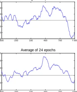
When both conditions are met, we can assume that by averaging of sufficient number of epochs becomes background EEG signal close to zero at every point, while the ERP waveform stays almost unchanged. The average of 8, 16 and 24 epochs can be seen in Figure 4.3. It is clearly visible that the noise becomes more and more suppressed as the number of epochs in average increase.

The averaged ERP waveform can be distorted even when both conditions are met. The main cause is usage of epochs with artefacts (e.g. eye blinks) that has significantly higher amplitude than EEG and ERP signal (200 µV). It is recommended to use any artefact detection method and exclude epochs contaminated with artefacts from averaging.

(19)

Figure 4.3: Example of the epoch averaging technique. All epochs belongs to the target stimulus. It is clearly visible that the noise is more suppressed as the number of epochs in average increase. Also the P300 component becomes visible by eye.

4.5. Artefact Processing

An artefact detection is crucial part in epoch preprocessing, because epochs damaged by artefacts significantly change the epoch average and thus make the ERP detection harder. Artefacts are typically very large compared to the ERP signal and may greatly decrease the S/N ratio of the averaged ERP waveform [4]. This problem becomes even bigger in the case of single trial detection where each epoch is classified instead of classification of the epoch average.

There are two main classes of techniques for eliminating the deleterious effects of artifacts. First, it is possible to detect large artifacts in the single-trial EEG epochs and simply exclude contaminated trials from the averaged ERP waveforms (this is called artifact rejection). Alternatively, it is sometimes possible to estimate the inﬂuence of the artifacts on the ERPs and use correction procedures to subtract away the estimated contribution of the artifacts (this is called artifact correction). [4]

4.5.1. Artefact Rejection

An artefact rejection process is a signal detection problem when signals (trials) are classified into two classes – epochs with and without artefacts.

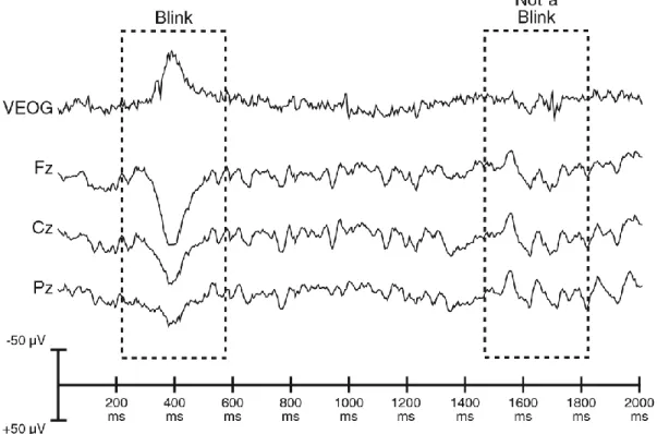
Artefacts with typically high amplitude (e.g. eye blinks) are mostly detected by simple subtraction of the baseline from the highest peak of the trial. Artefact is detected when this subtraction exceeds chosen threshold. An alternative approach is to measure the difference between minimum and maximum voltages within an epoch and again compare this value to the threshold. Both methods should be applied to EOG epochs instead of EEG epochs. The eye blink response consists primarily of a monophasic deﬂection of 50–100 mV with a typical duration of 200–400 ms. Perhaps the most important characteristic of the eye blink response, however, is that it is opposite in

-500 -200 100 400 700 1 000 -60 -40 -20 0 20 40 60 80 100 First epoch -500 -200 100 400 700 1 000 -60 -40 -20 0 20 40 60 Average of 8 epochs -500 -200 100 400 700 1000 -40 -20 0 20 40 60 Average of 16 epochs Time (ms) A m p litu d e  V -500 -200 100 400 700 1000 -40 -20 0 20 40 60 Average of 24 epochs

(20)

Page 16 polarity for sites above versus below the eye (compare, for example, the VEOG and Fz recordings in Figure 4.4) [4].

It is crucial to choose the threshold value carefully. If low threshold level is chosen then all epochs with eye blink artefact will be excluded from the averaging, but there will be a lot of false positive detection. It is possible that there will be not enough trials left for averaging and SNR of the average will be reduced. In the case of high threshold value, enough trials will remain in average, but many trials will contain blink artefact and the average will be probably distorted.

Several types of artefacts in the ERP technique can be easily removed just by simple filtering. EMG artefacts and 50/60 Hz power grid interference can be removed by using proper low-pass filter. EMG or heartbeat artefacts can be also detected or removed by using additional sensors on the body surface.

Figure 4.4: Recording of the vertical EOG (VEOG) electrode and Fz, Pz and Cz EEG electrodes. A

blink can be seen at approximately 400 ms, and it appears as a negative deﬂection at the VEOG electrode and as a positive deﬂection at the scalp electrodes. [4]

4.5.2. Artefact Correction

There are two serious reasons, why use artefact correction instead of artefact rejection. First, the rejection of large number of trials may lead to an unrepresentative sample of trials. Second, some subjects (patients) are not able to control their blinking and eye movement and it may be hard to obtain sufficient number of artefact-free trials.

The easiest way to correct eye artefacts is to compute the propagation between eye and EEG electrodes and subtract this value from each EEG channel. The most serious problem is that EOG contains also brain activity. Part of the brain activity is then removed from EEG channels. A newer approach is to use independent component

(21)

analysis (ICA). Several studies demonstrated that ICA is able to correct eye blinks, eye movement and electrical noise from the EEG signal [14, 15].

4.6. Statistical Analysis

Once the ERP waveforms are collected from a sample of subjects and amplitude and latency measures are obtained, it is time to perform a statistical analysis to see whether effects are signiﬁcant. The most recently used statistical method is ANOVA (Analysis of Variance). ANOVA is a univariate statistical method that tests difference between two or more groups.

Assumptions:

 Independent observations

 Normal distribution of dependent variable

 Homogeneity of variance

One way ANOVA has the following model:

𝑦ℎ𝑖 = 𝜇 + 𝛼ℎ+ 𝜀ℎ𝑖 (4.1)

𝑖 = 1,2, … , 𝑛ℎ, ℎ = 1,2, … , 𝐻,

where 𝛼_ℎ is an effect of h-level factor, 𝜀_ℎ𝑖 are random elements and 𝜇 is a constant. The main task of ANOVA is to compute P value of statistical test to accept or reject hypothesis.

First the total sum of squares is computed using the following equation

𝑄_𝑇 = ∑ ∑(𝑦_ℎ𝑖− 𝑦̅)2_(4.2)

𝑛𝐻

𝑖=1 𝐻

ℎ=1

Then the between group sum of squares is computed

𝑄_𝐵= ∑ ∑(𝑦̅_ℎ− 𝑦̅)2 ₌ 𝑛𝐻 𝑖=1 𝐻 ℎ=1 ∑ 𝑛_ℎ(𝑦̅ℎ− 𝑦̅)2 𝐻 ℎ=1 (4.3)

and the within group sum of squares

𝑄_𝐸 = ∑ ∑(𝑦_ℎ𝑖 − 𝑦̅_ℎ)2_. 𝑛𝐻 𝑖=1 (4.4) 𝐻 ℎ=1

Sums of squares are in the following relationship:

𝑄_𝑇 = 𝑄_𝐵+ 𝑄_𝐸. (4.5)

Finally the P value can be acquired using the formula

𝑃2 ₌𝑄𝐵

𝑄𝑇 ∈ 〈0,1〉. (4.6)

The closer the 𝑃2 value to 1 is, the bigger the difference between groups. The recommended threshold value of 𝑃2 is 0.05 [4]. This threshold means that there is a 95% probability that the similarity between groups is not a coincidence.

(22)

Page 18

5. Time-frequency Domain Methods for ERP Detection

5.1. Wavelet Transform

Wavelet transform (WT) is a time-frequency domain method for analysis and processing of nonstationary signals such as EEG. Both Continuous Wavelet Transform (CWT) and Discrete Wavelet transform (DWT) are suitable for EEG/ERP signal processing. The basic idea of wavelet transform is to decompose the input signal into a set of basis functions called wavelets [16]. This is done by scaling and dilatation of a prototype wavelet called the mother wavelet by the following equation:

Ψ𝑎,𝑏(𝑡) =

1 √𝑎Ψ (

𝑡 − 𝑏

𝑎 ), (5.1)

where Ψ is the analyzing wavelet, 𝑎 is the scaling factor, and 𝑏 is the time shift. 5.1.1. Continuous Wavelet Transform

The continuous wavelet transform of a signal f for the dilatation a and the translation b

of the wavelet ψ is defined in [17] as follows:

𝑊𝑇(𝑓, 𝑢, 𝑠) = ∫ 𝑓(𝑡) +∞ −∞ 1 √𝑎Ψ ( 𝑡 − 𝑏 𝑎 ) 𝑑𝑡 (5.2)

The CWT algorithm can be performed in four steps:

1) A mother wavelet, starting and ending value of dilatation, step of dilatation, and translation are set.

2) Sum of values of correlation for current dilatation and for every translation step to cover the whole signal is computed.

3) The value of dilatation is increased by the dilatation step. The algorithm continues with step 2)

4) The calculation is stopped when maximum value of dilatation is reached.

The result of CWT is usually visualized in a grayscale (the highest values are white) scalogram (Figure 5.1) in which each coefficient represents a degree of correlation between the transformed wavelet and the signal.

(23)

5.1.2. Discrete Wavelet Transform

The most commonly used algorithm is the Discrete Wavelet Transform (DWT), which has the linear computational complexity. It is based on the restricting position and scales. [19]

Instead of using a continuous wavelet function as in CWT, DWT uses two discrete signals – wavelet and scaling functions. Given the limited spectrum band of wavelet functions, the convolution process with this function can be interpreted as a limited band-pass filter [20]. In terms of digital signal processing, wavelet transform can be considered as a bank of filters with signal decomposition into sub-frequency bands. The slowest fundamental frequency components are detected using a scale function. Wavelet function is then documented by a high pass filter and the scale function is a complementary low pass filter. Relevant coefficients are determined taking the convolution of signal and the corresponding analyzing function [18, 20]. The scale is inversely proportional to the frequency; the low frequencies correspond to large scales and to the dilated wavelet function. Using the wavelet analysis at large scales, we obtain global information from the signal (an approximate component). At small scales we obtain detailed information (a detailed component) representing rapid changes in the signal [21].

Calculation of DWT coefficients is implemented by a gradual application of the wavelet function (high frequency filter) and scale function (low frequency filter) to the given signal using Mallatov decomposer scheme (see Figure 5.2). For each level of decomposition p so-called detailed component 𝐷_𝑝(𝑛) of the input signal is the output of the high pass filter ℎ_𝑑(𝑘). The approximation component𝐴_𝑝(𝑛) is the output of low the frequency filter 𝑙_𝑑(𝑘). Using the convolution and the subsequent subsampling the following equations are valid [21]:

𝐷𝑝(𝑛) = ∑ ℎ𝑑(𝑘)𝐴𝑝−1(2𝑛 − 𝑘) 𝐿−1 𝑘=0 (5.3) 𝐴_𝑝(𝑛) = ∑ 𝑙𝑑(𝑘)𝐴𝑝−1(2𝑛 − 𝑘) 𝐿−1 𝑘=0 (5.4)

for 𝑛 = 0, … , 𝑁/2, where 𝐴₀(𝑛) = 𝑥(𝑛) is the analyzed signal, and both sequences

(24)

Page 20

Figure 5.2: Principle of discrete wavelet transform [18]

5.1.3. ERPs detection with WT

When we look for the ERP waveform we compute correlation between a wavelet (which is scaled to correspond to the ERP waveform) and the EEG/ERP signal in the corresponding part of the signal, where the ERP waveform could be situated. This approach avoids a false ERP waveform detection in the signal parts which couldn’t contain the ERP waveform. Wavelet coefficients are affected by the match of scaled wavelet and the signal and also by the signal amplitude. When the degree of the correlation is higher than an established threshold, the ERP waveform is considered to be detected. [22]

Wavelet coefficients can be also used as features for any classification algorithm (e.g. Multi-layer Perceptron or Support Vector Machines). In [23] the P300 component was successfully detected in single-trial detection. The Daubechies 8 mother wavelet was used to extract features from the input signal. After DWT was performed, 16 approximation coefficients of level 5 for each channel was stored in 1-dimensional array and used for subsequent classification. Figure 5.3 shows how the DWT coefficients were obtained from the input data.

(25)

Discrete wavelet transform coefficients DWT output (512) cA5 (16) cA5 (16) cD5 (16) cD4 (32) cD3 (64) cD2 (128) cD1 (256) Ep o ch ( 5 1 2 s am p le s) cA1 cD1 cD2 cA5 cA5 cA2 cD4 cA4 cA3 cD3 cD5

Figure 5.3: DWT coefficients. Input EEG signal has 512 samples. The number of coefficients

obtained by DWT is in brackets. 5-level DWT was performed. cA1 - cA5 represent approximation coefficients of different levels, cD1 - cD5 represent detail coefficients. [23]

5.2. Matching Pursuit

The main idea of the Matching Pursuit (MP) algorithm is to decompose a signal into a sum of waveforms called atoms that are selected from a dictionary. The atom that has the highest scalar product with the original signal is chosen in each iteration. This atom is subtracted from the input signal and the residue enters the next iteration of the algorithm. The total sum of atoms selected successively in algorithm iterations is an approximation of the original signal. The more iterations is done, the more accurate approximation is obtained [24].

The dictionary of Gabor atoms is typically used. Suppose a Gaussian window g defined as follows:

𝑔(𝑡) = 𝑒−𝜋𝑡2_(5.5)

Then the Gabor atom has the following deﬁnition:

𝑔_{𝑠,𝑢,𝑣,𝑤}= 𝑔 (𝑡 − 𝑢

𝑠 ) 𝑐𝑜𝑠(𝑣𝑡 + 𝑤), (5.6)

where s means scale, u latency, v frequency and w phase. These four parameters deﬁne each individual atom.

An output of the MP algorithm is a good input for classifier but it is not suitable for visual inspection of a scientist. The output of the MP algorithm is usually visualized by the Vile transformation for this purpose. You can read more about a Winger-Vile transformation in e.g. in [25].

5.2.1. Usage of Matching Pursuit for ERP detection

The trend of the signal is approximated in first iterations whereas the signal details are approximated in later iterations. The major part of the ERP waveform should form a significant part of the signal trend. We typically know the latency of waveform that we are looking for. So we search for a Gabor atom which position corresponds to ERP’s latency and which approximates well the trend of the signal.

(26)

Page 22

5.3. Hilbert-Huang Transform

The Hilbert-Huang transform (HHT) is a signal processing method that decomposes signal into a set of so-called intrinsic mode functions (IMFs). The algorithm is designed to process non-stationary signals and was later modified to process an EEG/ERP signal. HHT consists of two algorithms – empirical mode decomposition and Hilbert spectral analysis (HSA). The EMD decomposes a signal into IMFs. The IMF is a function which fulfills the following condition:

 The mean value of the envelope defined by the local maxima and the local minima is zero at any point [26, 27, 28].

HSA applies the Hilbert transform on every IMF and allows us to compute the signal instantaneous attributes. The original HHT is not fully suitable for the ERP detection because the EEG signal is quasi-stationary. The EMD algorithm creates envelopes around the processed signal. This process suffers from an over/undershoot effect. The over/undershoot effect slows down the convergence of the EMD and causes the distortion of created IMFs.

5.3.1. Empirical Mode Decomposition

The most important part of the HHT is the EMD algorithm. The goal of the EMD is to decompose signal into IMFs and the residue. EMD is a data driven method and IMFs are derived directly from the signal itself [29]. IMF represents a simple oscillatory mode as a counterpart to a simple harmonic function, but it is much more general: instead of constant amplitude and frequency, as a simple harmonic component, the IMF can have a variable amplitude and frequency as the function of time [30]. The core of the EMD is the sifting process that acquires a single IMF from the signal. EMD starts with the original (preprocessed) signal. In the sifting process we look for local extrema (minima and maxima) in the input signal and we create upper and lower envelopes by connecting local extrema with a cubic spline. Then we calculate the mean curve by averaging the upper and lower envelopes and subtract the obtained mean curve from the input signal. Finally, if a stopping criterion is met, we have found an IMF and the sifting process ends. In other case the sifting process continues with the next iteration. After acquiring an IMF the sifting is finished and the EMD continues with obtaining the residue by subtracting the IMF from the signal. If the residue has at least two extrema, we set the residue as the current input signal and continue with the next sifting process. Otherwise the EMD is over and we have a set of IMFs and the residue. This basic algorithm is usable for both a general non-stationary signal and an EEG signal. [31]

The stopping criterion (SC) controls the selection of IMF in the sifting process. As we are trying to fulfill the IMF condition, amplitude variations of the individual waves become more even. Therefore Standard deviation (SD) [27] or Cauchy convergence test (CC) [32] is usually used as the stopping criterion:

𝑆𝐷 = ∑|ℎ𝑘−1(𝑡) − ℎ𝑘(𝑡)|2 ℎ_𝑘−12 _(𝑡) 𝑇 𝑡=0 , (5.7) 𝐶𝐶 =∑𝑇𝑡=0|ℎ𝑘−1(𝑡) − ℎ𝑘(𝑡)|2 ∑𝑇 ℎ_𝑘−12 _(𝑡) 𝑡=0 . (5.8)

A function in the current iteration of the sifting process is considered to be IMF, when the value of the stopping criterion is smaller than a threshold. The threshold value is

(27)

selected empirically depending on the used stopping criterion and the experimental design.

Extracted IMFs are in most cases only approximations of IMFs, because it is very difficult to fulfill this condition strictly, it means to achieve the zero mean value of the envelope at any point. Two simple additional stopping criteria (ASCs) was designed to help the sifting process to select IMFs that better correspond to the signal trend. The first ASC, is a simple mean value of the mean curve (MV) [31]:

𝑀𝑉 =∑ 𝑥𝑖

𝑁 𝑖=1

𝑁 . (5.9)

The mean value of the mean curve created from envelopes is zero if the mean value of envelopes is zero at any point. The second ASC is called the dispersion from zero (ZD) [31]. It is based on a standard deviation:

𝜎 = √∑ (𝑥𝑖 − 𝑥̅)2

𝑁 𝑖=1

𝑁 . (5.10)

The standard deviation is a measure of the dispersion from the average. However, we are interested in how big dispersion from zero is, because the average of every IMF mean curve should be zero. We set 𝑥̅ to zero and we get the formula for the second ASC: 𝑍𝐷 = √∑ 𝑥𝑖 2 𝑁 𝑖=1 𝑁 . (5.11)

The sifting process extract IMF when both standard stopping criterion and ASC are met. A big problem of the EMD algorithm is named mode mixing. It is caused mainly by noise and intermittency. The intermittency is referred to as a component that comes into existence or disappears from a signal entirely at a particular time scale [33]. The mode mixing problem occurs when the frequency tracks of an IMF jump as an intermittent component arrives or departs. Extracted IMFs then lose their physical meaning.

The solution to this problem is called Ensemble Empirical Mode Decomposition (EEMD). EEMD is a noise-assisted data analysis method. EEMD adds a random white Gaussian noise to the signal and computes standard EMD. EEMD obtains IMFs by simple averaging of outputs of multiple EMDs. The main idea is that the white noise will disappear when sufficient number of IMFs with added white noise is averaged and only clean IMF will remain.

5.3.2. Empirical Mode Decomposition for multichannel data

The EMD algorithm is designed to process univariate data, but EEG recordings are essentially multivariate. The number of channels used may vary from one channel to several dozen. Scientists have published several new approaches to EMD to decompose multichannel data in last few years.

The first extension of EMD which operates fully in the complex domain was first proposed by [34], termed rotation-invariant EMD (RI-EMD). The extrema of a complex/bivariate signal are chosen to be the points where the angle of the derivative of the complex signal becomes zero, that is, based on the change in the phase of the signal. The signal envelopes are produced by using component-wise spline interpolation, and

(28)

Page 24 the local maxima and minima are then averaged to obtain the local mean of the bivariate signal. [35]

An algorithm which gives more accurate values of the local mean is the bivariate EMD (BEMD) [39], where the envelopes corresponding to multiple directions in the complex plane are generated, and then averaged to obtain the local mean. The set of direction vectors for projections are chosen as equidistant points along the unit circle. The zero mean rotating components embedded in the input bivariate signal then become bivariate/complex-valued IMFs. The RI-EMD and BEMD algorithms are equivalent for

K=4 direction vectors. [35]

An extension of EMD to trivariate signals has been recently proposed by [36]; the estimation of the local mean and envelopes of a trivariate signal is performed by taking projections along multiple directions in three-dimensional spaces. To generate a set of multiple direction vectors in a three-dimensional space, a lattice is created by taking equidistant points on multiple longitudinal lines on the sphere (obtaining the so-called ‘equi-longitudinal lines’). The three-dimensional rotating components are thus embedded within the input signal as pure quaternion IMFs, thus benefitting from the desired rotation and orientation modelling capability of quaternion algebra.

A new EMD algorithm was published for multivariate data processing. Multivariate Empirical Mode Decomposition (MEMD) is able to process multi-channel data such as EEG. The multivariate EMD algorithm has been recently proposed in [35] to process a general class of multivariate signals having an arbitrary number of channels. It extends the concept of BEMD and trivariate EMD by processing the input signal directly in a multidimensional domain (n-space), where the signal resides. To achieve that, input signal projections are taken directly along different directions in n-dimensional spaces to calculate the local mean. This step is necessary since calculation of the local mean, a crucial step in the EMD algorithm, is difficult to perform due to the lack of formal definition of maxima and minima in higher dimensional domains. [37]

5.3.3. Hilbert Transform

The set of extracted IMFs by any of the mentioned EMD algorithms is an input to the Hilbert transform (HT). HT computes an analytical signal

𝑍(𝑡) = 𝑋(𝑡) + 𝑖𝑌(𝑡) = 𝑎(𝑡)𝑒𝑖𝜃(𝑡)

for every IMF, where 𝑋(𝑡) is the real part that represents the original signal, and

𝑌(𝑡) is the imaginary part that represents the Hilbert transform of 𝑋(𝑡). The imaginary part contains original data with 90° phase shift. The analytical signal allows us to calculate signal instantaneous attributes:

𝑎(𝑡) = √𝑋(𝑡)2_{+ 𝑌(𝑡)}2_{, (5.13)}

𝜃(𝑡) = 𝑎𝑟𝑐𝑡𝑎𝑛 (𝑌(𝑡)

𝑋(𝑡)), (5.14) 𝜔(𝑡) = 𝑑𝜃(𝑡)

𝑑𝑡 , (5.15)

where 𝑎(𝑡) is the instantaneous amplitude, 𝜃(𝑡) is the instantaneous phase and 𝜔(𝑡) is the instantaneous frequency. The knowledge of amplitude and frequency is essential for ERP component detection.

(29)

5.3.4. ERP detection using HHT

After an EEG epoch is preprocessed the HHT can be applied to decompose the epoch into set of IMFs. Based on equations from chapter 5.3.2. the instantaneous signal attributes are computed for each IMF. Subsequent detection of an ERP waveform is based on knowledge of typical ERP’s frequencies and latencies. Both frequencies and latencies of waveforms of which the input EEG/ERP signal is composed from, does not disappear during the EMD process. They are only decomposed into IMFs – including frequencies and latencies ERPs are made of. The ERP waveform is detected at each extracted IMF around its expected position using a classifier or by a human expert.

MEMD is also suitable for denoising of ERP data. The background EEG signal was removed using MEMD in [38]. After data are channel-wise denoised, features can be extracted (e.g. instantaneous signal attributes described in section 5.3.3 or any other features) and ERP waveform can be detected by a classifier.

(30)

Page 26

6. ERP Detection Methods

6.1. Linear Classifiers

Linear classiﬁers use linear functions to separate classes. Let us focus on the two-class case and consider linear discriminant functions. Suppose we have N-dimensional feature space, a weight vector 𝝎 = [𝜔₁, 𝜔₂, … , 𝜔_𝑁] and a threshold 𝜔₀. Then the corresponding decision hypersurface is a hyperplane [40]:

𝑔(𝒙) = 𝝎𝑻_{𝒙 + 𝜔}

0 = 0 (6.1)

For any 𝒙𝟏, 𝒙𝟐 on the decision hyperplane, Equation 6.2 directly implies that the

diﬀerence vector 𝒙_𝟏− 𝒙_𝟐 (i.e. the decision hyperplane) is orthogonal to the vector 𝝎 [40].

0 = 𝝎𝑻_𝒙

𝟏+ 𝜔0 = 𝝎𝑻𝒙𝟐+ 𝜔0 ⟹ 𝝎𝑻(𝒙𝟏− 𝒙𝟐) = 0 (6.2)

The most popular linear classiﬁers for BCIs include Linear Discriminant Analysis and Support Vector Machines. [41]

6.1.1. Linear Discriminant Analysis

The Linear Discriminant Analysis (LDA, also known as Fisher’s LDA) is widely used linear classiﬁer and dimensionality reduction technique. The separating hyperplane is obtained by seeking the projection that maximize the distance between the two classes means and minimize the interclass variance [42]. To solve a N-class problem (N > 2), several hyperplanes are used. [41] This technique has a very low computational complexity which makes it suitable for on-line BCI systems. Furthermore, this classifier is simple to use and generally provides good results. [41]

For known Gaussian distributions with the same covariance matrix for all classes, it can be shown that Linear Discriminant Analysis (LDA) is an optimal classiﬁer in the sense that it minimizes the risk of misclassiﬁcation for new samples drawn from the same distributions. LDA is equivalent to Least Squares Regression. [18]

ERP waveform detection is easy. The first step is to obtain an N-dimensional feature vector from each epoch. Ten the feature vectors are manually divided into two classes – first containing the ERP waveform and second without ERP waveform. The LDA is computed and a hyperplane divides N-dimensional space into two subspaces. One subspace contains feature vectors of epochs which contain an ERP waveform. The other subspace contains all other feature vectors.

6.1.2. Support Vector Machines

A Support Vector Machine (SVM) classifier [43] uses a discriminant hyperplane to separate classes. The hyperplane is not unique and classiﬁer may converge to any possible solution. The selected hyperplane is the one that maximizes the margins, i.e., the distance from the nearest training points. Maximizing the margins is known to increase the generalization capabilities [44]. In Figure 6.1, the margin for direction “1” is 2zl and the margin for direction ”2” is 2z2. The goal is to search for the direction that gives the maximum possible margin. For any linear classiﬁer, the distance between a point and a hyperplane can be calculated using the following equation [44]:

𝑧 =|𝑔(𝑥)|

(31)

𝝎, 𝜔0can be scaled so that the value of g(x), at the nearest points in 𝜔1, 𝜔2 (circled in

Figure 6.1), is equal to 1 for 𝜔₁ and, thus, equal to -1 for 𝜔₂. Assuming these conditions, the following can be stated: [45]

 The margin equals: _‖𝜔‖1 +_‖𝜔‖1 =_‖𝜔‖2

 We require:

𝝎𝑻_{𝒙 + 𝜔}

0 ≥ 1, ∀𝒙 ∈ 𝜔1

𝝎𝑻_{𝒙 + 𝜔}

0 ≥ −1, ∀𝒙 ∈ 𝜔2

For each 𝒙_𝒊, we denote the corresponding class indicator by 𝑦_𝑖 (+1 for 𝜔₁, -1 for 𝜔₂). Our task can now be summarized as: compute the parameters 𝝎, 𝜔0of the hyperplane

so that to [44]:

 minimize 𝐽(𝝎) =1₂‖𝜔‖2

 subject to 𝑦𝑖(𝝎𝑻𝒙𝒊+ 𝜔0) ≥ 1

Obviously, minimizing the norm makes the margin maximum. This is a quadratic optimization task subject to a set of linear inequality constraints. [44]

If the data is not linearly separable, the formulation can be modified to become a soft-margin classifier. Misclassifications are now allowed with a given penalty that is regulated by the penalty parameter that must be chosen in advance. [46] SVMs are discussed in more detail in [44].

Figure 6.1: The ﬁgure depicts a linearly separable classiﬁcation problem. However, there are

multiple solutions for the decision hyperplane. The margin for direction 2 is larger than the margin for direction 1. Therefore, it is the preferable solution for the Support Vector Machine. [44]

(32)

Page 28

6.2. Neural networks

Neural networks as a typical representative of non-linear classiﬁers have non-linear decision boundaries. They may be superior to linear classiﬁers if the features are not linearly separable [45].

6.2.1. Perceptron

The perceptron [47] is the simplest artiﬁcial neural network. It represents an artiﬁcial

neuron and it simulates the functioning of a single biological neuron. The perceptron has the following deﬁnition:

𝑦 = 𝑓 (∑ 𝜔_𝑖𝑥_𝑖+ 𝜃

𝑛

𝑖=1

), (6.4)

where 𝑦 is the output of the neuron, 𝜔_𝑖 are weights of the neuron, 𝑥_𝑖 are inputs of the neuron, θ is the threshold and 𝑓 is the neural activation function. For a single perceptron, the learning algorithm gradually adjusts its parameters to increase the probability of correct classification in the next step. At the beginning, the weights are set to initial values, typically chosen by random. The weights are updated according to the classification error, i.e. the Euclidean distance between the real and expected output. The problem with the perceptron is that it finds a separating hyperplane but not the optimal one. The algorithm is based on the following steps [47]:

1. Weights and a threshold are initialized. Weights 𝜔_𝑖(0) and the threshold 𝜃 are set to random low values.

2. The pattern and expected output are accepted. The input vector 𝑿 =

𝑥₁, 𝑥₂, … , 𝑥_𝑛 is applied to the perceptron and the expected output 𝑑(𝑡), being either +1 or -1, is stored.

3. The current output is calculated as:

𝑦(𝑡) = 𝑓ℎ(∑ 𝜔𝑖(𝑡)𝑥𝑖(𝑡) − 𝜃 𝑛

𝑖=1

) (6.5)

with 𝑓ℎbeing threshold function returning -1 for any x < 0 and +1 for any x > 0.

4. The weights are updated:

𝜔𝑖(𝑡 + 1) = 𝜔𝑖(𝑡) + 𝜂[𝑑(𝑡) − 𝑦(𝑡)]𝑥𝑖(𝑡) (6.6)

with 𝑑(𝑡) being:

 +1, if the pattern belongs to the ﬁrst class

 - 1, otherwise

The constant η represents learning rate.

5. The process is iterated until stopping condition is fulﬁlled. After training, classiﬁcation is based on applying Step 3. [45]

The perceptron is important because many more complicated neural networks use the perceptron as a building block to build more complex structures.

6.2.2. Multi-layer Perceptron

Multi-layer perceptron (MLP) is a widely used neural network. It consists of two or more layers of perceptrons and follows a supervised learning model. From structural point of view, it is based on perceptrons connected in a form of more layers. The output

(33)

of each neuron is connected to all neurons from the next layer [47]. An example of classiﬁcation using MLP is shown in Figure 6.2.

Since one perceptron can classify using one decision hyperplane, two perceptrons in the same layer represent two hyperplanes. Adding an additional layer enables the neural network to separate a more complex shape. [47]

Backpropagation In the 80s, the discovery of backpropagation algorithm sparked a renewed interest in artificial neural networks. The algorithm is based on error minimization that leads to a gradual update of weights and thresholds. The parameters are updated starting from the last layer of MLP and finishing with the first layer. [47]

MLP for P300 BCIs Multi-layer perceptrons can approximate any continuous function. Furthermore, they can also classify any number of classes. This makes MLP very flexible classifiers that can adapt to a great variety of problems. Therefore, MLP, which are the most popular networks used in classification, have been applied to almost all BCI problems. However, the fact that MLP are universal classifiers makes them sensitive to overtraining, especially with such noisy and non-stationary data as EEG. Therefore, careful architecture selection and regularization is required. [48]

A successful single trial detection of the P300 component using MLP is described in [23].

Figure 6.2: The ﬁgure depicts how the ERPs can be classiﬁed using multi-layer perceptron. Feature

vectors are accepted with the input layer and propagated throughout the network. The decision about the class can be based on comparing the outputs of two output neurons, the higher output decides the class. [45]

(34)

Page 30 6.2.3. Deep Learning

Theoretical results suggest that in order to learn the kind of complicated functions that can represent high-level abstractions, one may need deep architectures. Deep architectures are composed of multiple levels of non-linear operations, such as in neural nets with many hidden layers or in complicated propositional formulae re-using many sub-formulae. Searching the parameter space of deep architectures is a diﬃcult task.

[49]

Deep learning methods aim at learning feature hierarchies with features from higher levels of the hierarchy formed by the composition of lower level features. Automatically learning features at multiple levels of abstraction allow a system to learn complex functions mapping the input to the output directly from data, without depending completely on human-crafted features. This is especially important for higher-level abstractions, which humans often do not know how to specify explicitly in terms of raw sensory input. [49]

Depth of architecture refers to the number of levels of composition of non-linear operations in the function learned. Whereas most current learning algorithms correspond to shallow architectures (1, 2 or 3 levels), the mammal brain is organized in a deep architecture [50] with a given input percept represented at multiple levels of abstraction, each level corresponding to a diﬀerent area of cortex. Inspired by the architectural depth of the brain researchers wanted to train deep multi-layer neural networks but without any successful attempt until 2006. Something that can be considered a breakthrough happened in 2006: Hinton et al. at University of Toronto introduced Deep Belief Networks (DBNs) [51], with a learning algorithm that greedily trains one layer at a time, exploiting an unsupervised learning algorithm for each layer, a Restricted Boltzmann Machine (RBM) [52]. [49]

Until 2006, deep architectures have not been discussed much in the machine learning literature, because of poor training and generalization errors generally obtained [53] using the standard random initialization of the parameters. Gradient-based training of deep supervised multi-layer neural networks, which starts from random initialization, often gets stuck in “apparent local minima or plateaus”, and that as the architecture gets deeper, it becomes more diﬃcult to obtain good generalization. Much better results gives approach, when all layers are pre-trained with an unsupervised learning algorithm, one layer after the other, starting with the ﬁrst layer.

Energy-Based Models and Boltzmann Machines

Energy-based models associate a scalar energy to each conﬁguration of the variables of interest [54, 55, 56]. Learning corresponds to modifying that energy function so that its shape has desirable properties. Energy-based probabilistic models may deﬁne a probability distribution through an energy function, as follows:

𝑃(𝒙) = 𝑒

−𝐸𝑛𝑒𝑟𝑔𝑦(𝒙)

𝑍 , (6.7)

i.e., energies operate in the log-probability domain. [49]

In many cases of interest, x has many component variables xi, and we do not observe of these components simultaneously, or we want to introduce some non-observed variables to increase the expressive power of the model. So we consider an observed part (still denoted x here) and a hidden part h