An improved bio-optical model for the remote sensing of
Trichodesmium
spp. blooms
T. K. Westberry and D. A. Siegel
Institute for Computational Earth System Science, University of California, Santa Barbara, California, USA
A. Subramaniam
Lamont-Doherty Earth Observatory, Columbia University, Palisades, New York, USA
Received 2 June 2004; revised 15 January 2005; accepted 10 March 2005; published 25 June 2005.
[1] The cyanobacteriumTrichodesmium spp. can be an important ecological and biogeochemical component for both the coastal and open ocean ecosystems by way of its nitrogen fixation ability. However, information regarding its spatial and temporal distribution remains sparse.Trichodesmiumhas unique optical properties that should allow for its spectral signature to be detectable in satellite ocean color data sets. Here, a global data set of concurrent measurements of Trichodesmiumabundance and radiometric reflectance was compiled and used to develop bio-optical models forTrichodesmium. The most robust global model related the water-leaving radiance signal to the identification of an occurrence of a Trichodesmium bloom above a threshold value of 3200 trichomes L1. Using the in situ data set, this model is trained to successfully predictTrichodesmium blooms (92%) while minimizing false positive retrievals (16% of nonbloom
observations). A validation of the approach applied to Sea-viewing Wide Field-of-view Sensor (SeaWiFS) ocean color imagery shows that the model correctly predicts 76% of the bloom occurrences of an independent validation data set of in situ Trichodesmium observations. Ultimately, maps ofTrichodesmiumbloom occurrence will provide a means of addressing the ecology ofTrichodesmiumand its contribution to new production of the world oceans.
Citation: Westberry, T. K., D. A. Siegel, and A. Subramaniam (2005), An improved bio-optical model for the remote sensing of
Trichodesmiumspp. blooms,J. Geophys. Res.,110, C06012, doi:10.1029/2004JC002517.
1. Introduction
[2] Nitrogen fixation in the world oceans has received
increasing attention in the recent decade due to revised rate estimates which imply significant contributions to regional and global biogeochemical cycling of carbon and nitrogen [Michaels et al., 1996;Gruber and Sarmiento, 1997;Karl et al., 1997;Capone et al., 1997].Trichodesmium, a colonial, filamentous cyanobacterium, appears responsible for a large portion of this N2fixation (although the recognized
phylo-genetic groups that contribute to global N2 fixation are
becoming more diverse [e.g.,Zehr et al., 2001]). Observa-tions of the spatial and temporal distribution of these organisms on regional and global scales are sparse, despite being studied for several decades now. They are universally distributed throughout the tropical and subtropical oceans, yet the transient nature ofTrichodesmiumblooms has made their study difficult. As a result, present quantitative esti-mates of Trichodesmium abundance and its associated N2
fixation rates still have a large degree of uncertainty in them.
[3] Satellite remote sensing methods provide great
poten-tial for making large-scale estimates of Trichodesmium
abundance on regional to global scales. Previous attempts at developing empirical algorithms for discriminating Tri-chodesmium have worked well on the data they were developed from, but as of yet, no globally applicable bio-optical algorithm relatingTrichodesmiumto satellite remote sensing measurements exists. Trichodesmium have unique optical properties that should allow them to be detected from satellite orbit including (1) increased absorption in the near-UV and blue portion of the spectrum due to high amounts of associated colored dissolved organic matter (CDOM) [Steinberg et al., 2004], and water-soluble, UV-absorbing pigments [Subramaniam et al., 1999a], (2) higher relative reflectance near 570 nm due to phycoerythrin fluorescence [Borstad et al., 1992; Subramaniam et al., 1999b], and (3) increased backscatter across all wavelengths caused by the index of refraction change within intracellular gas vacuoles [Borstad et al., 1992; Subramaniam et al., 1999b]. It is thought that each of these features should be manifest in an ocean reflectance spectrum when Trichodes-miumis present in sufficient quantities, such as that under bloom conditions. Although they generally exist in low background concentrations, episodic blooms of extremely high concentration have been observed (106 trichomes JOURNAL OF GEOPHYSICAL RESEARCH, VOL. 110, C06012, doi:10.1029/2004JC002517, 2005
Copyright 2005 by the American Geophysical Union. 0148-0227/05/2004JC002517
L1 [Devassy et al., 1978; Creagh, 1985; Carpenter and Capone, 1992, and references therein]), albeit never with direct radiometric measurements. A satellite based method for estimating the presence of Trichodesmium blooms would provide an ideal way to estimate the biogeochemical impact of these blooms.
[4] Here, we compiled all available concurrent
radiomet-ric measurements and equivalent indices ofTrichodesmium
abundance to evaluate past Trichodesmium-specific bio-optical models and to develop new methods. As a result, an inverse semianalytic ocean color model, adapted from
Garver and Siegel [1997], is used to provide a determi-nation of the Trichodesmium-specific chlorophyll concen-tration, Chltri. This model is capable of indicating the
presence or absence of equivalent Trichodesmiumbiomass above a threshold value (3200 trichomes L1) with a high degree of fidelity. The model is validated when applied to the Sea-viewing Wide Field-of-view Sensor (SeaWiFS) ocean color data set using independent observations of
Trichodesmiumabundance. Last, an example of application to SeaWiFS ocean color imagery is shown to demonstrate the utility of the model in assessing aspects of the ecology of Trichodesmium.
2. Methods
2.1. Field Observations of Reflectance and TrichodesmiumAbundance
[5] Coincident measurements of ocean optical properties
and Trichodesmium abundances were compiled from a number of cruises throughout the subtropical oceans from 1994 to present (Table 1). Some were collected as part of large-scale oceanographic programs (e.g., Bermuda Atlantic time series, Atlantic Meridional Transect, NSF Biocomplex-ity, N2 fixation, etc.) while others came from individual
Trichodesmium oriented research expeditions. Each record in this data set contains corresponding estimates of in situ above water, spectral remote sensing reflectance,Rrs(0
+
,l),
Trichodesmium abundance, and phytoplankton chlorophyll
a concentration, chl a(N = 130). Remote sensing reflec-tance was calculated for the six SeaWiFS wavebands (412, 443, 490, 510, 555, and 665 nm) as Rrsð0þ;lÞ ¼ 1r n2 Luð0;lÞ Edð0;lÞ ; sr1 ð1Þ
where r is the average specular reflectance at the sea surface,3%Austin[1974], andnis the index of refraction of seawater, taken as 1.341. Lu(0, l) is the spectral
upwelling radiance just beneath the sea surface measured by a profiling spectroradiometer, andEd(0+,l) is the incident
spectral irradiance above the sea surface measured by a similar radiometer in air. All measurements and calculations adhere to the SeaWiFS ocean optics protocols [Mueller et al., 2002].
[6] Trichodesmium collection and enumeration was
per-formed slightly differently among the various cruises. In general, a full Niskin bottle (12 L) of seawater was collected near the surface and gravity filtered through 10 mm mesh. The filter contents were preserved with low-concentration Paraformaldehyde (2 – 4%) and Tricho-desmiumabundance was determined by epifluorescent mi-croscopy. The other method employed was collection via a plankton net outfitted with a flowmeter (usually 202 mm mesh). The net was deployed for a specified length of time and colonies were picked from the cod end, preserved and counted as above. All values are nominal surface values, but are taken anywhere from 0 – 5 m depth. For standardization purposes, colony abundances were converted to equivalent trichomes per liter using a value of 200 trichomes col1 [Carpenter, 1983]. In addition, chlorophyllaconcentrations were determined either fluorometrically or via HPLC pig-ment analysis and represents bulk phytoplankton chloro-phyll. Trichodesmium-specific chlorophyll, Chltri, was
estimated from trichome abundance using values of 50 ng chlacol1[Carpenter, 1983].
2.2. Satellite Observations and an Independent Validation Data Set
[7] An independent data set of Trichodesmium
observa-tions was used to validate the accuracy of our approach when applied to satellite imagery. Reflectance spectra,
Rrs(0+, l), were provided from SeaWiFS normalized
water-leaving radiance determinations. Spectra were extracted from level 3 GAC data with 9 km resolution at times and locations collocated with the Trichodesmium
observations. Of the 142 matchups, 77 were satellite overpasses during the shipboard observations described in the previous section. The remaining 65 were additional
Trichodesmiumabundance estimates without in situ radiom-etry. Together, these data constitute a second independent data set of matched Trichodesmium-Rrs(0+, l) suitable for
model validation purposes. The satellite determined reflec-tance spectra were quality controlled by excluding observa-tions where the atmospheric correction may be suspect. In particular, pixels with the aerosol model spectral slope greater than 1.1 (i.e., e78 > 1.1) or an aerosol optical
thickness spectral slope greater than 0.5 (i.e., A˚510 > 0.5) Table 1. Sources of Data for In Situ (N = 130) and Satellite Data Set (N = 142) and Ranges of Trichodesmium Abundance and In Situ Bulk Chl-a
Date Location Trichodesmium, trichomes L1 Chl-a, mg m3 Na Reference
Sept. 1994 Sargasso Sea 0 – 12 0.06 – 0.26 13 unpublished
Nov. 1999 Arafura/Timor Sea 146 – 11,071 0.06 – 0.82 26 (28)
April 1998 southwest Pacific 879 – 6293 0.09 – 0.11 3 (54)
Jan. 2001 tropical Atlantic 66 – 2339 0.01 – 0.22 14 (8) Capone et al.[2005]
July 2001 tropical Atlantic 21 – 73 0.03 – 0.04 26 (15) Capone et al.[2005]
Aug. 2003 Sargasso Sea 0 – 1426 0.00 – 2.68 26 (26) unpublished
1995 – 1999 tropical Atlantic 0 – 2860 0.11 – 0.30 22 (11) Tyrell et al.[2003] aNumbers in parentheses are cloud-free observations in satellite data set.
were discarded. This screening process eliminated nine additional paired measurements.
2.3. Trichodesmium-Specific Reflectance Model [8] The bio-optical model of Garver and Siegel [1997]
and Maritorena et al. [2002] was extended to retrieve
Trichodesmium abundances. In this framework, Rrs(l) is
related to the absorbing and backscattering properties of the water, or Rrsð Þ ¼l X2 i¼1 gi bbð Þl bbð Þ þl að Þl i : ð2Þ
Absorption,a(l), and backscatter,bb(l), coefficient spectra
can be decomposed into additive components including
Trichodesmium:
að Þ ¼l awð Þ þl aphð Þ þl acdmð Þ þl atrið Þl ð3aÞ
bbð Þ ¼l bbwð Þ þl bbpð Þ þl bbtrið Þl: ð3bÞ
Here, the subscripts w, ph, p, cdm, and tri refer to the absorption and backscattering due to water, phytoplankton, total particulates, colored dissolved and detrital matter, and
Trichodesmium, respectively. Each component is then
parameterized by a series of known or proscribed spectral shapes and unknown magnitudes:
aphð Þ ¼l Chla*phð Þl; ð4Þ
atrið Þ ¼l C1Tria*trið Þl; ð5Þ
acdmð Þ ¼l acdmðloÞexp½SðlloÞ; ð6Þ bbpð Þ ¼l 0:416 Chl0:766 0:002þ0:02 0ð :50:25 log ChlÞ 550 l ; ð7Þ
bbtrið Þ ¼l C2Tribb*trið Þl; ð8Þ
where the unknown quantities are; Chl, the chlorophyll a
concentration, Tri, the Trichodesmium abundance in trichomes L1 andacdm(lo), the absorption by CDM at a
scaling wavelength (lo = 443 nm). In practice, the Trichodesmium abundance is equated to Trichodesmium -specific chlorophyll using constant values of 50 ng chl a
col1 and 200 trichomes L1 [Carpenter, 1983]. Several quantities are specified in the model including the chlorophyll specific phytoplankton absorption spectrum, Figure 1. Chlorophyll-specific absorption and backscattering spectra included in the model.
(a)Trichodesmium(bold line [Subramaniam et al., 1999a]), ‘‘other’’ phytoplankton (dotted line [Bricaud et al., 1998]). (b)Trichodesmium(bold line [Subramaniam et al., 1999b]), ‘‘other’’ particulates (dashed line [Morel and Maritorena, 2001]), and water calculated as 0.5 total water scattering (dotted line [Smith and Baker, 1981]).
a* (phl) (taken fromBricaud et al.[1998]) andS, the spectral
slope of the CDM absorption curve [Maritorena et al., 2002]. The relationship describing particulate backscatter,
bbp(l) is taken from Morel and Maritorena [2001]. Trichodesmium chlorophyll-specific absorption and back-scattering spectra were taken from Subramaniam et al.
[1999a, 1999b]. These values are shown spectrally in Figure 1. Upon substitution, equation (2) can be inverted and solved by nonlinear least squares techniques for the three unknown quantities, Chl, Tri and acdm(lo). The
coefficients,C1andC2, were added to modify the amplitude
ofTrichodesmiumabsorption and backscatter to account for potential differences in the bio-optics between laboratory observations of Subramaniam et al. [1999a, 1999b] (Table 2) and field populations of Trichodesmium as well as for uncertainties in the conversions used to relate
Trichodesmium-specific chlorophyll concentration, tri-chome abundance and colony abundance. Optimization of these coefficients is described in a later section.
3. Results and Discussion
3.1. Data
[9] The distribution of Trichodesmiumabundance in the
present data set ranges from 0 to 11000 trichomes L1, with a mean value of2100 trichomes L1(Figure 2a). How-ever, values are not normally distributed about the mean and the median is significantly different (1250 trichomes L1)
suggesting that the infrequent large blooms dominate the statistics of the data set. Over 50% of the observations are less than 100 trichomes L1 and 75% are below 1000 trichomes L1. The upper range of this data set can be described as a very diffuse to a moderate sized bloom [Carpenter and Capone, 1992]. Nonetheless, the maximum values in this data set are much lower than previous estimates made under heavy bloom conditions (e.g., 106trichomes L1 [Devassy et al., 1978; Creagh,
1985;Carpenter and Capone, 1992, and references therein]). The associated in situ determined chlaconcentrations are log-normally distributed between 0.01 and 1.3 mg m3 (mean chla0.2 mg m3(Figure 2b)). These values are surprisingly low given the amount of Trichodesmium
biomass present. For example, the highest abundances of
Trichodesmiumin the present data set (104trichomes L1) should have chlorophyllaconcentrations of nearly 3 mg m3, if average values of 50 ng chlaper colony and 200 trichomes per colony are used [Carpenter and Romans, 1991;
Subramaniam et al., 1999a, 1999b].
[10] The reflectance spectra associated with the above
Trichodesmiumand chlorophylladistributions are shown in Figure 2c. There is a large degree of variability, especially at the blue end of the spectrum, but in general, Rrs(0+, l)
values are higher at shorter wavelengths (l < 500 nm) primarily due to the low chlorophyll concentrations present. The upper 10th percentile of the chlorophyll a
distribution exhibit slightly ‘‘green-shifted’’ spectra, but are
Table 2. Parameter Values and Sources Used in Final Model Formulation
Name Description Units Value or Source
aw absorption by water m1 Pope and Fry[1997]
a*ph Chl-specific phytoplankton absorption m
2
mg Chl1 Bricaud et al.[1998]
a*tri Chl-specificTrichodesmiumabsorption m2mg Chl2 Subramaniam et al.[1999a]
bbw backscattering by water m1 Smith and Baker[1981]
bbp particulate backscattering m1 Morel and Maritorena[2001]
bb*tri Chl-specificTrichodesmiumbackscatter m2mg Chl2 Subramaniam et al.[1999b]
S spectral slope of CDM absorption Maritorena et al.[2002]
C1 adjustment forTrichodesmiumabsorption 0.7097
C2 adjustment forTrichodesmiumbackscatter 0.2864
Figure 2. Distribution of observations in the pairedTrichodesmiumand in situ radiometric data set (N= 130). (a)Trichodesmiumabundance (trichomes L1). (b) Chlorophyll-a concentration (mg chlam3). (c) Above water, spectral remote sensing reflectance (sr1). Bold lines in Figures 2a and 2b are cumulative distribution function.
not associated with the higher Trichodesmium records (hchl ai = 0.55 ± 0.65 mg m3, hTrichodesmiumi = 146 ± 294 trichomes L1). Further, many of the hypoth-esized features of Trichodesmium dominated reflectance spectra described in the introduction are not observed.
[11] Figure 3 shows several mean spectra with different
optical origins for comparison. Both the mean of the entire data set and the mean of the upper 10th percentile of the Trichodesmium distribution are shown and differ only slightly from other spectra. The mean for 6 years of data (1992 – 1997) collected in the Sargasso Sea is also shown and represents an extreme example of very ‘‘blue’’ or optically clear water. The mean of the SeaBAM data set [O’Reilly et al., 1998] sampled for the same chloro-phyll distribution as this data (0 – 1.3 mg m3) represents a global average spectrum. The Trichodesmiumspectra do not appear unlike those of the SeaBAM data set, occu-pying roughly the same range of Rrs(0+, l) if the
chlorophyll distributions are matched. In addition, two model-derived spectra are shown, one containing Tricho-desmium [Subramaniam et al., 2002] and the other no
Trichodesmium (Hydrolight 4.1 [Mobley, 1994]), with Chltri= 1.0 mg m3and Chl = 1.0 mg m
3
, respectively. All of the data derived spectra are very similar throughout most of the visible spectrum, diverging near the blue end of the spectrum, and are very different than the two model derived spectra. The Rrs(0
+
, l) with higher asso-ciated Trichodesmium abundance (>1000 trichomes L1) appear slightly less ‘‘blue’’ than the rest of the
observa-tions, but not significantly different (95% confidence) than the mean SeaBAM Rrs(0+, l) at five out of six
wavelengths.
3.2. Previous Bio-optical Models forTrichodesmium [12] A handful of empirical bio-optical models describing
Trichodesmiumhave been developed during the past decade [Dupuoy et al., 1988; Borstad et al., 1992;Subramaniam and Carpenter, 1994; Tassan, 1995; Subramaniam et al., 1999b, 2002]. While each has its merit, only a few of these models can be used to provide a quantitative
measure of Trichodesmium abundance. Dupouy [1992] described ‘‘discolored’’ waters in the South Pacific as seen in true color CZCS imagery. The discoloration was as-sumed to be Trichodesmium by inference, although there was no ground truth data available. Borstad et al. [1992] showed that as the amount of Trichodesmium increased, the shape and magnitude ofRrs(l) changed, but provided no
way of linking the two.Subramaniam and Carpenter[1994] developed a proxy for the presence of Trichodesmium
in CZCS scenes, but it only provided a relative index of Trichodesmium influence on the reflectance from a pixel.
[13] Only Subramaniam et al. [2002] presents a
quan-titative means of estimating the amount of Trichodesmium
biomass present from a given Rrs(l). In this approach a
forward remote sensing reflectance model in combination with select SeaWiFS scenes created a set of criteria for screening pixels containing Trichodesmium that were Figure 3. Mean above water spectral remote sensing reflectance for various cases: present in situ
observations (bold line),Trichodesmiumobservations >1000 trichomes L1(dotted line), SeaBAM data (dashed line), Bermuda 1992 – 1997 (dash-dotted line),Subramaniam et al.[2002] model (circles), and non-TrichodesmiumCase I water model (solid line).
validated against shipboard observations. These criteria tested SeaWiFS, nLw(l) for certain shape and magnitude
characteristics and therefore, allowed the spatial extent of a bloom to be mapped. An empirical relationship then quantified the amount of Trichodesmium-specific chloro-phyll relative to total chlorochloro-phyll as estimated by the operational SeaWiFS algorithm. If we test the Rrs(0+, l)
[or equivalent nLw(l)] spectra in the data set presented here, we find that none meet any of the criteria set forth, much less all three simultaneously, as is the requirement to be flagged as Trichodesmium (results not shown). This failure is not entirely unexpected as the criteria were partially developed from satellite radiances, unlike the manner of past chlorophyll algorithm building which relies on in situ data [O’Reilly et al., 1998]. The mis-match of scales between in situ measurements and the satellite radiometry was noted by Subramaniam et al.
[2002] although no data was available to address this issue. Differences could also be the result of mixed optical assemblages, or the fact that the method of
Subramaniam et al. [2002] was developed using only a few SeaWiFS scenes of a single bloom event which might not be representative of the optical variability of Tricho-desmium in the natural environment.
[14] Although several of the past modeling approaches
have shown how Rrs(0+, l) can be influenced by Tricho-desmium, the diagnosis of a relationship is not always straightforward. It is easily seen how similar the associ-ated Rrs(0+, l) estimates can be to more typical
oligotro-phic and mesotrooligotro-phic waters, while still containing ‘‘significant’’ amounts of Trichodesmium. Figure 3 very clearly shows that existing bio-optical approaches would not be able to distinguish Trichodesmiumfrom moderately elevated ‘‘bulk’’ chlorophyll. It is likely true that at higher abundances, Trichodesmium would significantly alter the remote sensing reflectance spectrum and take on the expected spectral shape and magnitude characteristics that have been hypothesized [i.e., Borstad et al., 1992;
Subramaniam et al., 2002]. However, while this may be true for large monospecific blooms, mixed phytoplankton assemblages, and thus mixed optical signatures are probably the rule rather than the exception. The modeled spectra of Subramaniam et al. [2002] demonstrate such a case (Figure 3).
[15] The few independent estimates of Trichodesmium
Rrs(l) produced by either model or measurement do show
familiar Rrs(l) spectra at lowerTrichodesmium abundance
[Borstad et al., 1992; Subramaniam et al., 1999b].
Borstad et al. [1992] showed hypothesized reflectance spectra and in situ measurements of Rrs(l) at varying Trichodesmium abundances. Measurements made at the lowest concentrations in their dilutions (46,000 tri-chomes L1) were 4 times greater than the largest values reported here (11,000 trichomes L1), yet show only the slightest indication of expected Trichodesmium character-istics [see Borstad et al., 1992, Figure 6]. In fact, if the
Rrs(l) shown by Borstad et al. [1992] were extrapolated
toTrichodesmiumdensities similar to those in the data set presented here, they would be in good agreement with measurements presented here (not shown). This can also be seen to a lesser extent in Subramaniam et al. [1999b] which shows very similar Rrs(l) between Trichodesmium
and other phytoplankton at low to moderate chlorophyll concentrations.
3.3. Application of a Semianalytical Bio-optical Model [16] Semianalytic ocean color models relate the remote
sensing reflectance, Rrs(0+, l), to the inherent optical
properties. The model of Maritorena et al. [2002] enables the simultaneous retrieval of the chlorophyll a concentra-tion, the absorption coefficient due to colored dissolved and detrital matter (CDM),acdm(lo), and particulate backscatter, bbp(lo), wherelo= 443 nm. On the basis of laboratory and
field measurements, it seems reasonable that Trichodes-mium populations will exhibit traits that will enable its remote estimation using this model. Up to 80% of the internal cell volume comprises gas vacuoles [Walsby, 1992; Borstad et al., 1992], resulting in very high back-scatter due to the large difference in index of refraction between water, cytoplasm, and the air within the vacuoles. Also, high abundances ofTrichodesmiumleech significant quantities of CDOM, some in the form of micosporine-like amino acids [Steinberg et al., 2004; Subramaniam et al., 1999a]. These properties should act to increase both
bbp(443) andacdm(443).
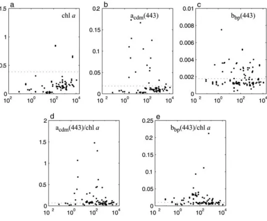
[17] Application of this model to the in situ data set
enables the analysis of these properties as a function of
Trichodesmium abundance as well as a comparison to a nominal ‘‘reference’’ state, calculated as the mean for the SeaBAM data set over the same chlorophyll range as the in situ data set (Figure 4). The SeaBAM data set likely contains few, if any, Trichodesmium observations and represents a globally representative (nonpolar) data set. Mean values for acdm(443) and bbp(443) are 0.018 and
0.0018 m1, respectively. While retrieved values of
acdm(443) andbbp(443) are at times 4 – 10 times higher than
the SeaBAM mean values, they are not necessarily associ-ated with high Trichodesmium observations. The same is true for determinations of acdm(443) and bbp(443) per unit
chlorophyll (m2mg chl a1). In short, there is no obvious pattern in any of these quantities, precluding their use as predictors ofTrichodesmiumbiomass.
3.4. Trichodesmium-Specific Model Tuning
[18] The initial Trichodesmium bio-optical model
(pre-sented in section 2.3) hindcast skill is very poor (r2= 0.08, RMSE = 0.70, bias > 104). This is not surprising, as the model coefficients have been optimized using a mostly
non-Trichodesmium data set [see Maritorena et al., 2002]. Consequently, a heuristic iterative approach [Press et al., 1990] was applied to determine optimal values for many or all of the parameters, and constitutes a simple ‘‘tuning’’ of the model. In this scheme, a cost function was defined and values of model parameters were drawn from a bounded random normal distribution, applied in the model, and the cost function evaluated (approach followsMaritorena et al.
[2002]). Those parameter sets resulting in local minima of the cost function were considered as ‘‘optimized coeffi-cients.’’ The form of the cost function chosen reflects the qualities of the model which were to be emphasized. It initially included standard metrics such as r2, RMS error, and normalized mean bias between observed and modeled abundance ofTrichodesmiumtrichomes. Free parameters to be optimized includedC1,C2, andS. Each of the candidate
models were tuned as described above. The number of iterations was dependent on the number of free parameters and ranged from 5 104to 1.6 105and spanned a factor of 3 (300% variability) in each respective parameter space. Although there was improvement in model success upon tuning, a viable 1:1 relationship was not realized (r2< 0.3 in all cases).
[19] The failure to capture a significant amount of
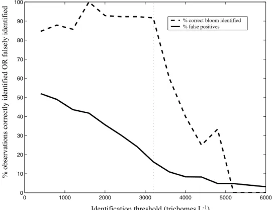
vari-ability inTrichodesmiumabundance led to a reconsideration of goals and to the assessment of where and when Tricho-desmium blooms occur and not their level. This casts the cost function in terms of correct and incorrect model estimates (false positive) above some ‘‘bloom’’ threshold, also called ‘‘commissions’’ and ‘‘omissions’’ byBrown and Yoder [1994]: CF¼ 1 #correct bloom #bloom observations þ #incorrect nonbloom #nonbloom observations:
Hence there are only two levels which can be confidently appointed, ‘‘bloom’’ or ‘‘nonbloom’’. In turn, the identifica-tion threshold was determined by a compromise between the values of the two terms in the cost function, the number of omissions and commissions. As the identification
threshold increases, the percentage of false positive retrievals decreases, yet the number of correct bloom predictions also decreases (Figure 5). That is, as we define a bloom at higher Trichodesmium abundance, there is obviously more margin for error at subbloom values (i.e., less false positives). However, we also have less and less bloom observations to tune the model with. A bloom value of 3200 trichomes L1 was chosen and represents a reasonable benchmark for bloom conditions. The best candidate model required optimization of only C1and C2
resulting in values of 0.7097 and 0.2864, respectively. Figure 6 shows observedTrichodesmiumabundance versus modeled abundance using the optimizedC1andC2with a
bloom threshold of 3200 trichomes L1. The model correctly identifies 92% of ‘‘bloom’’ observations and 84% of ‘‘nonbloom’’ observations, or 16% false positive retrievals in the in situ data set.
[20] An independently derived data set of satellite
Rrs(0+, l) from SeaWiFS (section 2.2) and collocated Trichodesmium observations were used to validate the model. Applying the model correctly identifies 76% of bloom observations and 71% of nonbloom observations (Figure 6). While this is not as good as the in situ results, most of the bloom values are correctly classified. The number of false positive retrievals is larger than expected (29%), but some of these could be excluded using differ-Figure 4. Optical property retrievals using the model of Maritorena et al. [2002] for the paired
Trichodesmium and radiometric observations (N = 130): (a) Chl a (mg m3); (b) acdm(443) (m1);
(c) bbp(443) (m1); (d) a*cdm(443) (m2mg chl1); and (e) bb*p(443) (m2 mg chl1). Horizontal dotted
lines represent mean retrieved values for the SeaBAM data set (fromO’Reilly et al. [1998]).
ent filters. A filter for suspect atmospheric correction was already applied to these data (as described in section 2.2) and flags a handful (N= 9) of the false positive retrievals. While this process improves the model statistics in this data set only slightly, a preliminary analysis of SeaWiFS images processed with the model described here show that this procedure successfully eliminates 5 – 10% of all bloom retrievals. In addition, it appears that some fraction of the false positives occur as isolated pixels with no other positive bloom retrievals in the immediate vicinity (not shown). These too, could be eliminated by applying a morphological erosion filter [e.g., Brown and Yoder, 1994]. Lastly, discrimination based on ecological indica-tors may also be possible. Trichodesmium blooms are known to occur in warm surface waters (>25C) and generally under low-wind conditions. By setting thresholds in these and other quantities (PAR, water depth, etc.) pixels could be masked before application of the model. This could effectively limit the number of potential false positive retrievals even further.
[21] The failure to yield absolute Trichodesmium
abun-dance estimates is unfortunate as this would allow better resolution in much of the ocean which undoubtedly falls below bloom conditions. Nonetheless, it is instructive to explore the cause of the model’s inability to achieve such a relationship. While it may be sufficiently easy to distin-guish large discolored patches of water from the surround-ings [e.g., Dupouy, 1992], natural variability in individual bloom characteristics prevents a scalable relationship to
predict the precise amount of Trichodesmium. Some of these characteristics have been noted and are related to age and health of the bloom. Changes in pigmentation of the community accompany the evolution of a bloom and the effects are not well understood. Borstad et al. [1992] summarize bloom reports in different growth stages and in different regions of the world as gray, reddish brown, greenish yellow, pale brown, and milk colored. This is a much wider range of optical variability than most phyto-plankton taxonomic groups. In addition to the color of a bloom, vertical position in the water column will change the surface reflectance. Though high-light-adapted and buoyant, Trichodesmiumis found throughout the euphotic zone, and small vertical changes in position can greatly alter satellite visibility. This becomes important as the water-leaving radiance signal is a depth-integrated mea-surement. Clayton [2001] used a numerical model to describe the relationship between bloom intensity and depth and the reflectance at the surface. The author found that Trichodesmium near the surface would only be detected in a reflectance signal if concentrations were greater than 1.5 mg chl a m3 (6000 trichomes L1).
Further, this detectability decreases rapidly with depth and becomes invisible at the surface even under extreme bloom conditions at 20 m depth. Using criteria similar to
Subramaniam et al. [2002] it was also shown that only 25% of observations collected on a cruise in the North Atlantic were detectable even though biomass was rela-tively high [Hood et al., 2001].
Figure 5. Terms of cost function (CF) as a function ofTrichodesmiumidentification threshold. Plotted are % correct bloom retrievals (dashed line) and % false positives (solid line) versus Trichodesmium
abundance (trichomes L1). Can also be thought of as (1 – % omissions) and % commissions, respectively.
Figure 6. Model estimates of Trichodesmium versus observed values (in units of trichomes L1). Correct prediction horizons are bounded by shaded boxes. Two data sets are shown. Circles are in situ data used to develop the model (i.e., hindcasts); 92% of bloom values are correctly identified, and 16% of nonbloom are observations incorrectly identified (N = 130). Crosses are model predictions from Sea Wide Field-of-view Sensor (SeaWiFS)-derived reflectances; 76% of bloom values correctly identified, and 29% of nonbloom observations are incorrectly identified (N= 133).
Figure 7. Positive Trichodesmium bloom retrievals using SeaWiFS imagery for a single 8 day composite (10 – 17 February 1998, 0.25resolution). Shown are a (sub)-tropical view (35N – 35S) and three regional extracts highlighting areas of activity: Gulf of Mexico/Caribbean, Indian Ocean/Arabian Sea, and the western Pacific/Indonesia.
[22] Other sources of uncertainty in the model could
stem from variability in the amount of chl a per colony and the number of trichomes per colony. Both are well documented and undoubtedly alter the remote sensing reflectance spectrum for a given Trichodesmium abun-dance. The degree of colony self-shading will also affect
Rrs(0+, l). This will be a function of bloom density and
morphology, themselves a function of bloom age. There are a number of physiological and ecological factors that cumu-latively make the model best as a binary indicator of the presence or absence ofTrichodesmiumblooms rather than an algorithm for the accurate determination of its biomass. 3.5. Application to Ocean Color Imagery
[23] A single SeaWiFS 8 day composite (10 – 17 February
1998, 0.25 resolution) was chosen to demonstrate the utility of the proposed model. Normalized water-leaving radiances were extracted from the image after undergoing standard SeaWiFS processing. These were converted to Rrs(0, l) and applied to the model, along with the
atmospheric screening described above. Results are shown in Figure 7 and include a near-global view (30N – 30S) and three enlarged subregions. The scale is rather large, and it is difficult to see individual or small groups of pixels (a larger image can be viewed on the web along with other examples at http://www.icess.ucsb.edu/toby/ tmp/Figure7.png). However, a very cursory examination of the image reveals a few interesting observations. Very few pixels give positive retrievals, in this image only 1.3% or 6700 out of 518,400 are above the identification thresh-old (3200 trichomes L1). In contrast the method of
Subramaniam et al.[2002] only detects 218Trichodesmium
pixels, and 122 of the same pixels. Second, clusters of positive bloom retrievals are not consistent with large-scale oceanographic features, such as those seen in chlorophyll images. Open ocean areas do not seem to have large organized blooms, but likely support subbloom concentra-tions of Trichodesmium (if any). The three zoom maps highlight the areas of greatest retrievals in this image; the Gulf of Mexico and Caribbean, the Arabian Sea, and broad areas of the western Pacific in and around many of the archipelagos there. Some of these areas have observed blooms reported in the literature [Devassy et al., 1978;
Carpenter and Romans, 1991, and references therein]. The average SeaWiFS chlorophyll in theTrichodesmiumbloom pixels is 0.23 mg m3, compared to a mean of 0.12 mg m3 for all noncloudy, nonbloom pixels. However, issues of self-shading within colonies become relevant and must be accounted for [Borstad et al., 1992; Subramaniam et al., 1999b]. Detailed analysis of the spatial and temporal patterns seen in this image and their relation to coincident environmental factors are beyond the scope of this paper, and this single image represents only a brief snapshot of the transient bloom field.
[24] In any event, the sparse nature of the retrievals will
make interpretation of maps such as this one difficult. In addition, the space and timescales of the satellite radiances might not match those ofTrichodesmiumbloom dynamics. A multiscale (both space and time) approach will be required to sufficiently characterize the extent of blooms. Additional parameters describing the physical environment at the global scale will be needed as well (i.e., sea surface
temperature, wind speed, mixed layer depth, irradiance, etc.). These and other problems will have to be addressed in order to fully exploit the usefulness of the model.
[25] Acknowledgments. The authors would like to acknowledge support from NASA and NSF in the form of an Earth System Science Fellowship (Toby Westberry) and the NSF-funded Biocomplexity-Nitrogen Fixation program, respectively. We would also like to thank two anony-mous reviewers and an editorial review that greatly improved the manu-script. Thanks to Doug Capone, Ed Carpenter, Norm Nelson, Debbie Steinberg, Toby Tyrell, and Karen Orcutt for contributing data.
References
Austin, R. W. (1974), The remote sensing of spectral radiance from below the ocean surface, inOptical Aspects of Oceanography, edited by N. G. Jerlov and E. Steemann Nielsen, pp. 317 – 344, Elsevier, New York. Borstad, G. A., J. F. A. Gower, and E. J. Carpenter (1992), Development of
algorithms for remote sensing of Trichodesmium blooms, inMarine Pelagic Cyanobacteria: Trichodesmium and Other Diazotrophs, edited by E. J. Carpenter and D. G. Capone, pp. 193 – 210, Springer, New York. Bricaud, A., A. Morel, M. Babin, K. Allali, and H. Claustre (1998), Variations of light absorption by suspended particles with chlorophyllaconcentration in oceanic (case 1) waters: Analysis and implications for bio-optical models, J. Geophys. Res.,103, 31,033 – 31,044.
Brown, C. W., and J. A. Yoder (1994), Coccolithophorid blooms in the global ocean,J. Geophys. Res.,99, 7467 – 7482.
Capone, D. G., J. Zehr, H. Paerl, B. Bergman, and E. J. Carpenter (1997),
Trichodesmium: A globally significant marine cyanobacterium,Science,
276, 1221 – 1229.
Capone, D. G., J. A. Burns, J. P. Montoya, A. Subramaniam, C. Mahaffey, T. Gunderson, A. F. Michaels, and E. J. Carpenter (2005), Nitrogen fixation by Trichodesmiumspp.: An important source of new nitrogen to the tropical and subtropical North Atlantic Ocean,Global Biogeochem. Cycles,19, GB2024, doi:10.1029/2004GB002331.
Carpenter, E. J. (1983), Nitrogen fixation by marineOscillatoria( Tricho-desmium) in the world’s oceans, inNitrogen in the Marine Environment, edited by E. J. Carpenter and D. G. Capone, pp. 65 – 103, Elsevier, New York.
Carpenter, E. J., and D. G. Capone (1992), Significance ofTrichodesmium
blooms in the marine nitrogen cycle, inMarine Pelagic Cyanobacteria: Trichodesmium and Other Diazotrophs, edited by in E. J. Carpenter, D. G. Capone, and J. Rueter, pp. 211 – 217, Springer, New York. Carpenter, E. J., and K. Romans (1991), Major role of the cyanobacterium
Trichodesmiumin nutrient cycling in the North Atlantic Ocean,Science,
254, 1356 – 1358.
Clayton, T. D. (2001),Trichodesmiumspp.: Numerical studies of resource competition, carbohydrate ballasting, and remote-sensing reflectance, Ph.D. dissertation, 241 pp., Old Dominion Univ., Norfolk, Va. Creagh, S. (1985), Review of literature concerning blue-green algae of the
genusTrichodesmium,Bull. 197, 33 pp., Dept. of Conserv. and Environ., Perth, Australia.
Devassy, V. P., P. M. A. Bhattathiri, and S. Z. Qasim (1978), Trichodes-miumphenomenon,Ind. J. Mar. Sci.,7, 168 – 186.
Dupouy, C. (1992), Discoloured waters in the Melanesian archipelago (New Caledonia and Vanuatu): The value of the Nimbus-7 Coastal Zone Colour Scanner observations, inMarine Pelagic Cyanobacteria: Trichodesmium and Other Diazotrophs, edited by E. J. Carpenter, D. G. Capone, and J. Rueter, pp. 177 – 191, Springer, New York.
Dupuoy, C., Y. Dandonneau, and M. Petit (1988), Satellite detected cyano-bacteria bloom in the southwestern tropical Pacific,Int. J. Remote Sens.,
8, 389 – 396.
Garver, S. A., and D. A. Siegel (1997), Inherent optical property inversion of ocean color spectra and its biogeochemical interpretation: 1. Time series from the Sargasso Sea,J. Geophys. Res.,102, 18,607 – 18,625. Gruber, N., and J. L. Sarmiento (1997), Global patterns of marine fixation
and denitrification,Global Biogeochem. Cycles,11, 235 – 266. Hood, R. R., N. R. Bates, D. G. Capone, and D. B. Olson (2001), Modeling
the effect of nitrogen fixation on carbon and nitrogen fluxes at BATS,
Deep Sea Res., Part II,48, 1609 – 1648.
Karl, D. M., R. Letelier, L. Tupas, J. Dore, J. Christian, and D. Hebel (1997), The role of nitrogen fixation in biogeochemical cycling in the subtropical North Pacific Ocean,Nature,388, 533 – 538.
Maritorena, S., D. A. Siegel, and A. R. Peterson (2002), Optimization of a semianalytical ocean color model for global-scale applications, Appl. Opt.,41, 2705 – 2714.
Michaels, A. F., D. Olson, J. L. Sarmiento, J. W. Ammerman, K. Faning, A. H. Knap, F. Lipschultz, and J. M. Prospero (1996), Inputs, losses and transformations of nitrogen and phosphorous in the pelagic North Atlantic Ocean,Biogeochemistry,35, 181 – 226.
Mobley, C. D. (1994), Light and Water: Radiative Transfer in Natural Waters, Elsevier, New York.
Morel, A., and S. Maritorena (2001), Bio-optical properties of oceanic waters: A reappraisal,J. Geophys. Res.,106, 7163 – 7180.
Mueller, J. L., et al. (2002), Ocean optics protocols for satellite ocean color sensor validation, revision 3,NASA Tech. Memo., 210004, 308 pp. O’Reilly, J. E., S. Maritorena, B. G. Mitchell, D. A. Siegel, K. L. Carder,
S. A. Garver, M. Kahru, and C. McClain (1998), Ocean color chloro-phyll algorithms for SeaWiFS,J. Geophys. Res.,103, 24,937 – 24,953. Pope, R. M., and E. S. Fry (1997), Absorption spectrum (300 – 700 nm) of pure water: II integrating cavity measurements,Appl. Opt.,36, 8710 – 8723.
Press, W. H., S. A. Tuekolsky, W. T. Vettering, and B. P. Flannery (1990),
Numerical Recipes in C: The Art of Scientific Computing, Cambridge Univ. Press, New York.
Smith, R. C., and K. Baker (1981), Optical properties of the clearest natural waters,Appl. Opt.,20, 177 – 184.
Steinberg, D. K., N. B. Nelson, C. A. Carlson, and A. C. Prusak (2004), Production of chromophoric dissolved organic matter (CDOM) in the open ocean by zooplankton and the colonial cyanobacterium Trichodes-miumspp.,Mar. Ecol. Prog. Ser.,267, 45 – 56.
Subramaniam, A., and E. J. Carpenter (1994), An empirically derived pro-tocol for the detection of blooms of the marine cyanobacterium Tricho-desmiumusing CZCS imagery,Int. J. Remote Sens.,15, 1559 – 1569. Subramaniam, A., E. J. Carpenter, D. Karentz, and P. G. Falkowski (1999a),
Bio-optical properties of the marine diazotrophic cyanobacteria Tricho-desmiumspp.: I Absorption and photosynthetic action spectra,Limnol. Oceanogr.,44, 608 – 617.
Subramaniam, A., E. J. Carpenter, and P. G. Falkowski (1999b), Bio-optical properties of the marine diazotrophic cyanobacteriaTrichodesmiumspp.: II. A reflectance model for remote sensing,Limnol. Oceanogr.,44, 618 – 627.
Subramaniam, A., C. W. Brown, R. R. Hood, E. J. Carpenter, and D. G. Capone (2002), DetectingTrichodesmiumblooms in SeaWiFS imagery,
Deep Sea Res., Part II,49, 107 – 121.
Tassan, S. (1995), SeaWiFS potential for remote sensing of marine Tricho-desmiumat sub-bloom concentrations,Int. J. Remote Sens.,16, 3619 – 3627.
Tyrell, T., E. Maran˜o´n, A. J. Poulton, A. R. Bowie, D. S. Harbour, and E. M. S. Woodward (2003), Large-scale latitudinal distribution of Tri-chodesmiumspp. in the Atlantic Ocean,J. Plankton Res.,25, 405 – 416. Walsby, A. E. (1992), The gas vesicles and buoyancy ofTrichodesmium, in
Marine Pelagic Cyanobacteria: Trichodesmium and Other Diazotrophs, edited by E. J. Carpenter, D. G. Capone, and J. Rueter, pp. 141 – 162, Kluwer Acad., Norwell, Mass.
Zehr, J. P., J. B. Waterbury, P. J. Turner, J. P. Montoya, E. Omoregie, G. F. Steward, A. Hansen, and D. M. Karl (2001), Unicellular cyanobacteria fix N2 in the subtropical North Pacific Ocean,Nature,412, 635 – 638.
D. A. Siegel and T. K. Westberry, Institute for Computational Earth System Science, University of California, Santa Barbara, CA 93106-3060, USA. ([email protected]; [email protected])
A. Subramaniam, Lamont-Doherty Earth Observatory, Columbia Uni-versity, Palisades, NY 10964-1000, USA. ([email protected]) C06012 WESTBERRY ET AL.: REMOTE SENSING OF TRICHODESMIUM SPP. BLOOMS C06012