MSI_1709
The employment elasticity of the minimum wage
Is it just politics after all?
Is it just politics after all?
By Jesse Wursten∗Draft: August 24, 2017
The effect of minimum wages on employment is highly disputed. The main questions in the literature are on how to deal with spa-tial heterogeneity and dynamics. We use statistical (multi-factor error models) and economic (political ideology as control variable) methods to address the first. Furthermore, we extend the models to a dynamic setting to estimate more long term effects. We find that these enriched models all suggest there are no economically signif-icant negative employment effects atttached to moderate increases in the minimum wage.
JEL: J38, D22, C23
Keywords: minimum wage, cross-sectional dependence, labour pol-icy, political ideology, common correlated effects models, interac-tive fixed effects, dynamic factor models, employment elasticity, labour markets
Do higher minimum wages lead to higher unemployment? The effect of minimum wage policy on employment levels is one of the most heavily debated economic questions in both academic and public circles. Whether they can serve as policy tool against poverty or inequality hinges on the impact on job creation and destruction as raising them might just lead to fewer people earning more. Without a credible and broadly accepted estimate of
∗ Thanks to Michele Lenza, Philip Vermeulen, Peter Karadi and Peter McAdam from the European Central
Bank, Dirk Czarnitzki, Lara Cockx and Geert Dhaene from the KU Leuven, Otto Toivanen from Aalto university and the participants of the CISS 2017, in particular Mark Roberts (Penn State) and Bettina Peters (ZEW), for their comments and suggestions.
the employment elasticity of the minimum wage, the public debate remains dominated by anecdotal evidence and simplistic theories.
This deficiency is not due to a lack of interest - Neumark and Wascher (2006) reference over a hundred publications in their survey of recent developments in the literature. There is also an abundance of data, with publicly available employment data and over 200 federal and state minimum wage changes in the US. Rather, the issue is disagreement within the economic community on which methodology is best suited to unearth the employment effects of the minimum wage, where one side finds strong disemployment effects and the other does not. This has even led to suspicions of author bias on both sides (Neumark, 2001), where authors would predominantly publish papers confirming their previous results. Although we do not share those suspicions, we do note that it has introduced some strain in the minimum wage debate.
In this paper, we try to break through this stalemate in three steps. First, we show that the various estimation approaches differ mainly in how they attempt to deal with spatial heterogeneity (the presence of unobserved (regional) factors affecting both employment and minimum wages) and the intricate dynamics of employment adjustments. Second, we demonstrate that the current methods are special cases of the multifactor error structure framework, which was developed specifically to model such issues. This is particularly useful because the two estimation techniques it is associated with, the Common Correlated Effects models (Pesaran (2006), Chudik, Pesaran and Tosetti (2011)) and the Interactive Fixed Effects model (Bai (2009), Moon and Weidner (2017)) allow for very general forms of spatial heterogeneity (SH), being robust to both local and global unobserved shocks. We apply both to twenty-four years of restaurant employment data from the Quarterly Census of Employment and Wages (QCEW) and compare the results to estimates from the most common techniques used in the literature in both static and dynamic settings. In the final step, we argue that the different results found in the literature reflect heterogeneous changes in political ideology across states and provide empirical evidence to support that statement. We find that controlling for SH greatly diminishes the case for strong disemployment effects,
regardless of whether one does this through statistical methods (time trends, multifactor models) or by explicitly including political measures as control variables. These enriched models also perform better at the robustness checks.1
In doing so, we attempt to bridge the gap between the two camps that have formed in the literature. The first, originating in Neumark and Wascher (1992), uses traditional panel estimation techniques to analyse the impact of minimum wage hikes and finds significant negative impacts on employment, with elasticities in the order of -0.20, reaffirming older time series-based evidence (Brown, Gilroy and Kohen, 1982).2
The second deals with spatial heterogeneity by focusing on local variation, either looking at individual cross-state case studies (Card and Krueger (1994), ...) or pooling them to-gether in a regression discontinuity-like design (Dube, Lester and Reich (2010), henceforth DLR). Here, the evidence is rather inconclusive. Some case studies find negative employ-ment effects, some discover positive effects, in others employemploy-ment levels do not respond to minimum wage hikes at all. Even the overall tendency is disputed. DLR note that “On balance, case studies have tended to find small or no disemployment effects”, whereas the listing of case studies in Neumark and Wascher (2006) is definitely a mixed bag, with roughly an equal number of positive and negative employment effect findings.
Both impose fairly strict restrictions on the interplay between counties and the speed of the adjustment process. Case studies for example are generally based on surveys shortly before and after a legislative change. Implicitly, these studies assume firms do not make any adjustments in advance, despite the early announcement of minimum wage hikes. Additionally, any longer-term changes occurring after the second survey are lost. The regression discontinuity design put forward by DLR assumes counties are not affected by minimum wage and employment evolutions across the border, which at times represent the 1E.g. they predict more credible earnings elasticities and unlike the standard fixed effects models do not predict
significant employment losses in the finance and accounting sectors where less than 2% of workers earn up to 1.25 times the minimum wages.
2Were the US to adopt the ‘living wage’ of $15 instead of the current $7.25 per hour, this implies teenage
employment would drop by∼20%. It is of course likely that the response to minimum wage hikes is not linear, even if only because the share of the working force affected does not increase linearly. Hence, this example should be taken with the necessary grains of salt.
same city (e.g. Kansas City, MO and Kansas City, KS). The panel studies spearheaded by Neumark and Wascher (1992) typically include only state and time dummies - filtering out only time-invariant and nation-wide effects. On the contrary, the dynamic multifactor error models we propose allow for longer adjustment periods, filter out national and regional (up to very local) unobserved common factors and remain powerful even if there are no such factors (Eberhardt, Banerjee and Reade, 2010).
The remainder of this paper is structured as follows. Section I briefly describes the history of minimum wage research and illustrates the issues highlighted by the recent literature. Section II describes the data and institutional framework. In Section III we link the notion of spatial heterogeneity to multifactor error models and show how they generalise current estimation methods. Section IV illustrates how such models can be estimated consistently in static and dynamic settings. Section V presents the results across a wide set of estimators (traditional and novel). In Section VI, we use these results and the political ideology measure to reconcile the different outcomes present in the literature. Section VII provides robustness checks. Finally, Section VIII concludes.
I. Related Literature
In this section, we first focus on the broad development of the minimum wage literature and the issues encountered along the way.3
The time series literature kicked off with the development of the Kaitz index (Kaitz, 1970) which combined information on the level of the minimum wage and its expanding coverage (across sectors, gender and age) in one variable. The employment elasticities obtained were generally negative, in the range of -0.1 and -0.3 and statistically significant (Brown, Gilroy and Kohen, 1982). The downside of these studies is that they have relatively little identifying variation to work with as the federal minimum wage only changed once or twice a decade. As a result, these results are likely to be contaminated by unobserved macro-3For a full introduction to minimum wage research, we refer to Brown (1999) for the theoretical aspects and the
earliest empirical work (mainly time series and the first panel studies). Neumark and Wascher (2006) provides an extensive summary of the developments in the late 90’s and the early 2000’s, when the debate between the merits of panel studies and case studies erupted. Finally, Addison, Blackburn and Cotti (2015) provide a clear description of the most recent literature.
evolutions correlated with the minimum wage hikes. From a statistical perspective, these studies are also plagued by non-stationarity (Williams and Mills, 2001) and a tendency to detect spurious correlations.
The focus shifted to panel studies as more detailed data became available and states started topping the federal minimum wage. Neumark and Wascher (1992) exploit this variation in minimum wage regimes across states to corroborate the time series results, finding elasticities in the same -0.1 to -0.3 range. A first dissenting observation came from Card (1992), who finds that employment evolutions after a minimum wage hike were not affected by its initial bite.4
The claim that minimum wages do not lead to job losses really gained traction after a (now famous) survey of fast food restaurants in the New Jersey and Pennsylvania states (Card and Krueger, 1994). Comparing employment levels in the two states before and after a serious increase in the New Jersey minimum wage, they find no evidence of any adverse effects of the hike in New Jersey.
Many papers have debated these findings and the tide of case studies following in its wake.5 For the sake of brevity, we restrict ourselves to two remarks. First, an implicit assumption to justify the cross-border case study approach is that geographically close areas are very alike, and more so than geographically distant areas (or you would use those as control group), which sounds plausible at first, but finds no evidence in synthetic control group tests (Neumark, Salas and Wascher, 2014). Second, using neighbours as a control group is only valid if employment levels in the control group are not affected by the treatment group.6 However, Manning and Petrongolo (2011) show that local labour markets tend to overlap strongly, leading to ripple-on effects beyond the treated area. Indeed, it seems implausible that employers in Philadelphia, PA are unaffected by changing 4If minimum wages reduce employment, you would expect the effect to be larger in states where the fraction of
workers earning less than the new minimum wage is higher.
5E.g. Ropponen (2011) find that the effects vary strongly with the size of the restaurant, Neumark and Wascher
(2000) argue the Card & Krueger survey contained serious measurement error and find negative employment effects when they use payroll data instead.
6The link can be direct (minimum wages in NJ affecting employment in PA) or indirect (employment in NJ
conditions in the New Jersey cities just a few minutes away.
Dube, Lester and Reich (2010) generalise the case study approach by creating a panel of all county pairs crossing state borders and comparing employment evolutions across these borders. They argue that standard panel studies are vulnerable to spatial heterogeneity and that by restricting their analysis to very local variation, they are insulated from these unobserved regional differences. Using this contiguous border county pair method (CBCP) they find no evidence for disemployment effects. Although their approach filters out some of the idiosyncratic noise plaguing case studies, it is still vulnerable to some of the same issues - i.e. they impose that employment evolutions across county borders are uncorrelated and that nearby counties are better control groups than the US average.
The synthetic control group method (Abadie, Diamond and Hainmueller, 2010) is a second method to perform more robust case studies and is less vulnerable to the latter critique. Rather than hand picking a control group, it generates an articifial control group by averaging over multiple states. Similarity in the pre-treatment stage determines the weights. Dube and Zipperer (2015) generalise this approach to allow multiple cases to be evaluated together and apply it to the minimum wage puzzle. They find that while the wage and employment elasticities differ strongly across states, overall the effect on employment is indistinguishable from zero. The downside of this approach is that it requires a long pre-treatment period to calculate the weights. Any states where minimum wages change too frequently have to be discarded - the criteria used by the authors allow them to use just 29 of the 215 state minimum wage changes between 1979-2013. In that sense, it does not appear a very attractive method to analyse minimum wages in the US, given that it throws away over 85% of treatments.
One thing all these approaches have in common is that they control for spatial het-erogeneity through a very rigid structure. The panel models include just state and time dummies which filter out only time-invariant state characteristics and state-invariant aggre-gate trends. In the case studies and their generalisation in the CBCP method, the implicit assumption is that nearby counties are very similar, despite being subject to different state
laws. The synthetic control group method assumes states that were (observably) similar in the past remain so in the future. Due to the many changes in the minimum wage, this past is rather short from a macroeconomic perspective (five years).
The multi factor structure (MFS) framework we employ in this paper assumes instead that there is a (potentially large) number of time varying factors which affect the depen-dent variable (e.g. restaurant employment) differently in different states. No structure is imposed on the time factors, nor on the state ‘loadings’. In this sense, it can be seen as a combination of state and time dummies, without fully saturating the model (as would be the case with state-time pair dummies). In Section III we show that standard panel techniques are nested in the MFS framework. There are two ways to estimate MFS models. The first was introduced by Pesaran (2006) and is generally referred to as the Common Correlated Effects (CCE) model. It adds cross-sectional averages of all the variables to the regression equation, with separate coefficients for each panel unit. These averages proxy for the unobserved factors.
Alternatively, one can estimate the factors directly using the Interactive Fixed Effects (IFE) model (Bai, 2009). Totty (2015) takes a first step in applying these static models to the minimum wage quandary and find that the significant negative employment elas-ticities in the restaurant sector (and for teenagers) vanish once they control for spatial heterogeneity this way.
The estimators have been enriched to remain consistent in dynamic panels by Chudik et al. (2013), Chudik and Pesaran (2015) and Moon and Weidner (2017) (see Section IV). This is particularly relevant in the minimum wage setting where the potential importance of dynamics has been stressed many times (e.g. Baker, Benjamin and Stanger (1999), Neumark and Wascher (2006), DLR, Keil, Robertson and Symons (2001), Burkhauser, Couch and Wittenburg (2000)), with different timing assumptions frequently leading to opposite results.7
7It is perhaps also no coincidence that in the seminal Arellano and Bond (1991) paper introducing the
Arellano-Bond estimator, the authors use an estimation of the drivers of employment levels as their example to demonstrate the importance of properly factoring in dynamic elements.
Our paper expands on this literature in multiple ways. First, we bridge the gap between the econometric journals and applied work by implementing the various dynamic factor models. Second, we demonstrate how these factors models can be helpful in analysing the different results obtained with the standard estimators. Finally, we introduce a variable measuring the political ideology of US states over time (Shor and McCarty, 2011) that is highly influential in the political science field, but has not found its way to economics research. We argue that the heterogeneous evolution in political sentiment across the US is the omitted variable that drives the difference in employment elasticities observed in the literature.
II. The Data
We follow Dube, Lester and Reich (2010) in using data from the Quarterly Census of Employment and Wages (QCEW), known as the ES-202 program until 2003. Its earnings and employment records are based on administrative records related to unemployment insurance and cover∼97% of salaried workers in the United States.
In line with the literature, we focus on employment in the restaurant service sector (NAICS 7221 + 7222)8 as it employs a disproportionate share of minimum wage workers, with 30% earning within 10% of the minimum wage in 2006 (DLR). Additionally, the sector is present in every county, although the data might at times not be available for confidentiality reasons.9 It covers both traditional (full service) restaurants as well as (limited service) fastfood and takeout joints. The sector provided employment to 10 million people in 2016, of which 30% were fastfood and counter workers (average hourly wage: $9.57), 20% were waiters ($11.57), 16% cooks ($11.28) and 7% supervisors ($16.66). See Table 1 for a more complete breakdown.10
Our full sample runs from 1990-2013, representing 288 months of employment informa-8NAICS classification from 2002.
9The Bureau of Labor Statistics (BLS) suppresses industry-county specific values if the industry is so small in
that county the numbers might allow observations to be made on individual establishments.
10Based on the Occupational Employment Statistics database. Note that it uses the more recent 2012 NAICS
classification, hence the numbers might not exactly match the data used in the regression. There might also be variations over time.
Table 1—Occupational distribution of the restaurant sector workforce
Occupation # of employees % of restaurant Average hourly (abbreviated OCC titles) in restaurant sector employment wage (in $) Fastfood and Counter Workers 3,031,790 29.47 9.57 Waiters and Waitresses 2,105,830 20.47 11.57
Cooks 1,659,270 16.13 11.28
Supervisors 742,610 7.22 16.66
Food Preparation Workers 424,590 4.13 10.57
Dishwashers 376,130 3.66 9.97
Hosts and Hostesses 360,060 3.50 10.15
Cashiers 313,850 3.05 9.79
Attendants and Helpers 273,830 2.66 10.44
Bartenders 269,980 2.62 12.88
Sales Workers and Drivers 217,080 2.11 10.39 Food Service Managers 143,040 1.39 25.58
Assorted Managers 70,460 0.68 36.35
Others (bakers, cleaners, ...) 286,600 3.59 13.62
Based on data from the Occupational Employment Statistics database. The restaurant sector is defined as NAICS 7225 from the 2012 edition of the NAICS classification.
tion.11 In our baseline results, we follow the literature by using a balanced panel, retaining the 1293 out of 3142 counties that have data for the full time period. These counties rep-resented 88% of total non-farm employment in December 2013 (own calculations based on BLS data). This leaves us with 300 000 observations (out of more than half a million, see Section VII). The QCEW does not provide hours-worked information, only a headcount of filled positions. As a result, we are limited to discussing effects along the extensive margin.
Structured, regression-ready data on minimum wage levels was obtained from the per-sonal website of Ian Salas (Neumark, Salas and Wascher, 2014) and cross-checked with official data from the BLS and law (amendment) texts.12 In total, we observe 426 mini-mum wage changes (counted at the state level). States are free to set the minimini-mum wage at any level, as long as it equals or exceeds the federal minimum wage. Many have made use of this freedom: 238 of the observed changes are the result of decisions by the state legis-latures, the remaining 188 are adjustments to stay in line with the federal minimum wage. 11DLR use quarterly employment data. We find that all results are qualitatively similar regardless of the time
unit chosen (see Section VII).
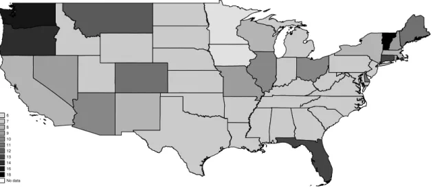
Figure 1. Frequency of minimum wages per state. Includes changes due to federal and state-level legislation. 6 7 8 9 10 11 12 13 14 16 18 No data
Figure 1 shows the geographical disparity in minimum wage change frequency, Figure 2 shows the evolution of minimum wages over time.
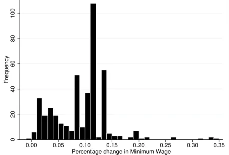
Not all minimum wage changes are made equal. The average increase of the mandated minimum wage was 9.5%, but this masks a wide variation in the size of the changes as depicted in Figure 3. About a quarter were smaller than 5%, often reflecting cost of living adjustments (by 2017, 18 states have pegged their minimum wage to some price index, usually the CPI). A handful of adjustments exceed 20%. Michigan spans the crown with their October 2006 increase of 35%. Colorado is the only state to have ever reduced the minimum wage (by 0.5% in 2010, following a decline of the consumer price index the year before).
III. Spatial Heterogeneity
The goal is to find the impact minimum wage legislation has on employment in the restaurant sector. In the simplest case, our regression equation could look like Equation 1, whereyit represents log of employment in the restaurant sector, αis a constant,xitis a
Figure 2. Evolution of minimum wages per state. 2 4 6 8 10
Minimum Wage (in $)
1990 1991 1992 1993 1994 1995 1996 1997 1998 1999 2000 2001 2002 2003 2004 2005 2006 2007 2008 2009 2010 2011 2012 2013 2014
Figure 3. Histogram of percentage minimum wage changes (1 percent bins).
0 20 40 60 80 100 Frequency 0.00 0.05 0.10 0.15 0.20 0.25 0.30 0.35 Percentage change in Minimum Wage
control variable, mwit is the log of the minimum wage andit is an error term.13 i and t identify the N counties (US) and T months. As employment and the minimum wage are both in logs, δ is an estimate of the employment elasticity of the minimum wage in the restaurant sector.
Unfortunately, it is highly unlikely that the combination of constant and control variable is enough to take care of spatial heterogeneity, i.e. that there are many unobserved factors that affect both the minimum wage and employment which vary over time (e.g. global food prices), across counties (climate) or both (local culture and institutions). A first option, illustrated in Equation 2, is to include county fixed effects, αi, and time fixed effects,
θt. These will only filter out time invariant county characteristics and county invariant aggregate shocks.
In Equation 3, we take it one step further by including state-specific time trends, γs∗t. Unlike time dummies, these control for unobserved characteristics that change over time at a different pace across US states.14 However, this specification is still very rigid, restricted to filtering out only linear trends. Especially in longer panels, this might not be satisfactory (e.g. business cycle and seasonality concerns).
yit=α+βxit+δmwit+it (1) yit=αi+θt+βxit+δmwit+it (2) yit=αi+θt+γs∗t+βxit+δmwit+it (3)
The multi factor stucture (MFS) illustrated in Equation 4 is more flexible and relaxes the linearity assumption while keeping the unit-specific impact. Ft= (f1,t, f2,t, ..., fR,t)0is a col-umn vector of R unobserved factors that change over time, whereasλi = (λ1,i, λ2,i, ..., λR,i)
13For ease of exposition we restrict ourselves to one covariate in this section. Expanding the logic to multiple
covariates is trivial.
14Or alternatively, factors that do not change over time, but permanently affect employment growth rather than
is a row vector of the respective factor loadings which differ across counties.15 These factor loadings reflect how each estimated factor affects the various counties. Note that both the fixed effects and the state specific time trend models are nested within this framework as illustrated in Equation 5 (where R = 3). For example, the county fixed effects can be represented as the combination of factor loading λ1,i = αi and ‘time variant’ factor
f1,t= 1. Likewise, the factor representing the state-specific trends is simplyf3,t =t. The corresponding factor loadings are identical for all counties belonging to the same state.16
yit=α+λ0iFt+βxit+δmwit+it (4)
yit=αi∗1 + 1∗θt+γs∗t+βxit+δmwit+it (5)
The flexibility of the MFS approach in terms of controlling for spatial heterogeneity comes from three separate sources: the county specific factor loadingsλi, the time variant factors Ft and the number of factorsR. This combination of multiple products of i and
t terms can capture very complex patterns in the data. That immediately raises the question of identification issues, which will be dealt with in the next section where we discuss estimation of MFS models.
IV. Estimation
There are many ways to estimate MFS models. We focus on two, the Interactive Fixed Effects (IFE) approach and the Common Correlated Effects (CCE) model because they allow the regressors to be correlated with the unobserved factors.17 This ability to reduce omitted variable bias is, for applied purposes, the main strength of these estimators.
15We refer to Section IV for a discussion on the number of factors R.
16The within-census division method advocated by Allegretto, Dube and Reich (2010), which includes census
division-time pair dummies can be written as an MFS model with one factor per census division (nine in total). The same goes for the CBCP method introduced by DLR, with one factor per cross-border county-pair (229 in our data). In practice, with that many factors, the employment elasticity of the minimum wage (δ) would not be properly identified anymore in either of the estimation methods we discuss in Section IV.
17The IFE estimator even allows for correlation with the loadings. The CCE model can be extended to allow the
We start with the Interactive Fixed Effects (IFE) approach, which treats the unobserved factors and their loadings as fixed parameters to estimate. Bai (2009) develops this method for static panels with large N and T. The intuition is fairly straightforward - suppose we have a linear regression setup such as Equation 4, with several regressors andRunobserved factors F, each with their unit-specific factor loading λ.18 Then the IFE estimator will alternate between two steps to find the solution to the least squares minimisation problem in Equation 6 (Λ = (λ1, λ2, ..., λN)). The objective function looks just like regular OLS, only with the factor term added. The two constraints ensure F and Λ are separately identified (Bai, 2009). (6) min β,F,Λ SSR= N X i=1 (Yi−Xiβ−F λi)0(Yi−Xiβ−F λi) subject to F0F/T =IR Λ0Λ is diagonal
Before the algorithm can kick off, it requires some (arbitrary) starting values for β, usually all the coefficients are set to one for the first run (step 0 in Equation 7). These are used to calculate the residuals Wi = Yi −Xiβ. The residuals are then subjected to principal component analysis, which provides an estimate of ˆF and ˆΛ (step A in Equation 8).19
In the second step, we update our estimate of ˆβ by regressing Xi on Yi −Fˆλˆi (the dependent variable minus the estimated factor term), which corresponds to step B in Equation 9. At this point, the algorithm reboots, using the new estimate of ˆβ to calculate the (factor-inclusive) residuals ˆWi in order to update the estimate of the factors and their loadings (step A). These estimates then lead to a new estimate of ˆβ (step B) and so on, 18To keep the notation clear, we group the control variables and minimum wage level in the (k×N×T) matrix X.
19Due to the two constraints in the minimisation problem, the factors in ˆFare the firstReigenvectors associated
with theRlargest eigenvalues of ˆWWˆ0, multiplied by√T. Correspondingly, ˆΛ = ˆW0F /Tˆ . See Bai (2009) for more details.
until the coefficient estimates change sufficiently little after each step.20
Step 0: βˆ(X) is set to arbitrary starting values (7) Step A: Fˆˆλi+i = ˆWi =Yi−Xiβˆ (8) Step B: βˆ( ˆF ,Λ) =ˆ N X i=1 Xi0Xi −1 N X i=1 X0(Yi−Fˆλˆi) (9)
The downside of Bai (2009)’s approach is that it assumes the regressors are strictly exogeneous with respect to the remaining error term (after the unobserved factors are filtered out), which rules out dynamic panels. In the dynamic case, we follow Moon and Weidner (2017), who start from a different set of assumptions to build up their estimator which allows them to include predetermined variables as regressors. In practice, their estimation procedure is identical to Bai’s, up until a bias correction term at the end, which corrects for correlation between regressors and past values of the error term (cfr. Nickell (1981)).21
Linking this back to the question at hand, this means we can consistently estimate Equation 10 and calculate the long run effect of the minimum wage on employment as
Pq
l=0δˆl/ 1−
Pp
l=1ρˆl
. It is generally more convenient to estimate Equation 11 instead, which explicitly imposes the presence of county and time fixed effects.
yit= p X l=1 ρlyi,t−l+ q X l=0 δlmwi,t−l+α+βxit+λ0iFt+it (10) yit= p X l=1 ρlyi,t−l+ q X l=0 δlmwi,t−l+αi+θt+βxit+λ0iFt+it (11)
20Some implementations then restart the process with different starting values for ˆβin order to reduce the
proba-bility of being in a local minimum. This is not the case for theregifecommand in Stata which we use for the static IFE estimates (Gomez, 2015), however the coefficients are identical to those obtained by the matlab code provided by Moon and Weidner (2017) which does support multiple runs.
21One small difference behind the scenes is that Moon & Weidner project ˆλand ˆF out ofX
iinstead of subtracting it. This speeds up convergence, but does not affect the final estimates.
Two issues remain to be discussed w.r.t. IFE estimation: the choice of number of factors
R and identification problems. First, Bai and Ng (2002) propose a barrage of tests to identify the true number of factors. They differ almost exclusively in the penalty attached to increasing the number of factors (relative to the decrease in the sum of squared residuals). The intuition is similar to traditional AIC and BIC model selection tests. Moon and Weidner (2015) argue that a consistent estimate ofR is not necessary, as long as one does not include too few factors (too many is not a problem). In the empirics, we follow their suggestion and err on the side of including too many factors, but show in the Appendix how the estimates change with the number of factors (see Section V).
As in traditional estimators, identification in IFE models depends on the degree of collinearity between the various components of the regression equation. Moon and Weidner (2017) distinguish between low- and high-rank regressors. The first vary almost exclusively in one dimension (e.g. a national price index by definition only varies over time), whereas the latter vary across both units (‘space’) and time. The minimum wage can be comfort-ably treated as a high-rank regressor as it differs in a non-systematic way across states and time. As a result, it is sufficient that the rank of the N ×T matrix of minimum wages (34) is larger than 2R+K1, whereK1 is the number of low rank regressors in the model. That condition ensures the factor cannot filter out all the variation in the regression and the minimum wage effect can still be identified as long as we keep the number of factors low enough (∼below 15).22 In practice, it is important to keep in mind that the factors try to explain the dependent variable, not the independent ones and therefore this rank condition is not an absolute limit.
The CCE models, introduced in Pesaran (2006), take a completely different approach. Instead of explicitly estimating the factors, the CCE method filters them out by including the cross-sectional averages of all variables. Equations 12 - 16 illustrate how this works with one factor (easily generalised).
22An intuitive interpretation of this condition is that the minimum wage variable should be sufficiently difficult
yit =βxit+δmwit+λiFt+vit (12) ¯ yt=βx¯t+δmw¯ t+ ¯λFt (13) ⇔Ft= ¯λ−1(¯yt−βx¯t−δmw¯ t) (14) ⇒yit =βxit+δmwit+λiλ¯−1(¯yt−βx¯t−δmw¯ t) +vit (15) ⇔yit =βxit+δmwit+π1iy¯t+π2ix¯t+π3imw¯ t+vit (16)
The barred variables represent the cross-sectional averages, ¯w = N−1PN
i=1wit. We
assume that ¯vt converges to zero asN goes to infinity and hence drops out leading to the expression in means in Equation 13. The equation is then inversed to show thatFtcan be represented as a transformation of the cross-sectional averages (Equation 14). Plugging this representation of Ft into the first equation leads to Equation 15, which can be estimated by OLS after a simple reparametrization (Equation 16).23 This estimator is known as the Common Correlated Effects Pooled model (CCEP).
The CCE framework can handle a fixed number of strong common factors and an infinite number of weak ones (Chudik, Pesaran and Tosetti, 2011) (strong factors affect many pan-els, whereas weak ones are more local shocks). Additionally, the estimator remains consis-tent under serially correlated errors and time-varying cross-sectional dependence (Pesaran and Tosetti, 2011), non-stationary unobserved common factors (Kapetanios, Pesaran and Yamagata, 2011) and weakly cross-sectionally dependent innovations (Pesaran and Tosetti, 2011). Finally, Pesaran and Tosetti (2011) conclude that the CCE estimators are less bi-ased in the presence of spatial spillovers than classic spatial autoregressive (SAR) models based on theoretical arguments and Monte Carlo evidence.
There are multiple ways to extend this type of estimation to dynamic panels in order to consistently estimate Equation 11. The simplest is to add lags of the cross-sectional 23Do note that the rescaled factor loadings vary per panel unit. Hence, the number of parameters to estimate grows
multiplicatively with N (the number of panels) and k (the number of dependent variables). As a result, standard estimation commands can take forever. Fortunately, the alternative approach behind thereghdfecommand (Correia, 2014) in Stata handles these cases with ease, even as N or k get large.
averages as advocated by Chudik and Pesaran (2015) and illustrated in Equation 17. In this CS-ARDL approach,pT should be large enough to approximate the infinite lag poly-nomial (pT =∞), but small enough to ensure sufficient degrees of freedom for consistent estimation.24 We follow Chudik et al. (2013) in setting pT = T
1
3 rounded down, which balances both conditions.
yit= p X l=1 ρlyi,t−l+ q X l=0 δlmwi,t−l+βxit + pT X m=0 πi,1my¯i,t−m+ pT X m=0 πi,2mmwi,t−m+ pT X m=0 πi,3mx¯i,t−m+αi+θt+it (17)
The advantage of the CS-ARDL approach is that it is consistent even if the regressors are endogenous, but it is vulnerable to incorrect lag specification. Moreover, Nickell bias (Nickell, 1981) due to the inclusion of panel fixed effects and the cross-sectional averages might be an issue in panels where T is not large (Everaert and Groote, 2016). Chudik et al. (2013) develop a new technique, the CS-DL model, which is more robust to lag misspecification and also performs better in the context of residual serial correlation and breaks in the error process. In this estimator, the lags of the dependent and independant variables are replaced by those of the differenced regressors, as shown in Equation 18. The coefficientδthen directly estimates the long run impact of the minimum wage on restaurant employment. yit=δmwi,t+βxit + pT−1 X n=0 γi,1m∆mwi,t−n+ pT−1 X n=0 γi,2n∆xi,t−n+ + pT X m=0 πi,1my¯i,t−m+ pT X m=0 πi,2mmwi,t−m+ pT X m=0 πi,3mx¯i,t−m+αi+θt+it (18)
24It is not required thatp
The CCE models we considered so far imposed that the impact of the minimum wage on employment is identical across counties (slope homogeneity). However, Pesaran and Smith (1995) argues that such pooled estimators are biased if the true coefficients differ across units. Instead, he advocates running separate time series regressions for each group and averaging the unit-specific coefficients at the end (‘mean group’ estimation). Equations 19-21 show the mean group counterparts of the CCE models.
CCEMG yit=αi+βixit+δimwit+π1iy¯t+π2ix¯t+π3imwt+it (19) CS-ARDLMG yit=αi+ p X l=1 ρi,lyi,t−l+ q X l=0 δi,lmwi,t−l+βixit + pT X m=0 πi,1my¯i,t−m+ pT X m=0 πi,2mmwi,t−m+ pT X m=0 πi,3mx¯i,t−m+it (20) CS-DLMG yit=αi+δimwi,t+βixit + pT−1 X n=0 γi,1m∆mwi,t−n+ pT−1 X n=0 γi,2n∆xi,t−n+ + pT X m=0 πi,1my¯i,t−m+ pT X m=0 πi,2mmwi,t−m+ pT X m=0 πi,3mx¯i,t−m+it (21)
The final coefficient is the arithmetic average of the unit-specific estimates. In the static and CS-DLMG cases, this is simply δ = PN
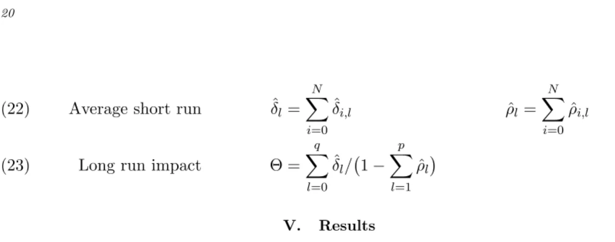
i=1δi/N. The CS-ARDLMG model is a bit more involved. We first obtain the average short run coefficients (Equation 22) and then calculate the long run coefficient using these averages (Equation 23).25
25It is also possible to calculate the county-specific long run coefficients first and then average those. This would
Average short run δˆl = N X i=0 ˆ δi,l ρˆl= N X i=0 ˆ ρi,l (22)
Long run impact Θ =
q X l=0 ˆ δl/ 1− p X l=1 ˆ ρl (23) V. Results
We apply these techniques to a balanced panel of total restaurant and fastfood employ-ment data between 1990 and 2013 in Tables 2 and 3. We add results obtained through the traditional estimators to ease comparison with the literature, as well as three statisti-cal tests to evaluate the fit of the model. The CD-test (Pesaran, 2004) tests for residual cross-sectional dependence (i.e. whether the residuals are correlated across counties), the LM-test (Born and Breitung, 2016) looks for serial correlation (correlation over time). A combination of the Hadri (Hadri, 2000) and Breitung (Breitung, 1999) tests is used to analyse whether the residuals are non-stationary (integrated of order > 0), which would question the interpretation of the coefficients as long run elasticities. All models contain total population, private sector employment and time dummies as first-line controls.
A. Static models
Table 2 reports the employment elasticity of the minimum wage in the restaurant sector for a variety of models. We find economically and statistically significant results only for the time fixed effects (TFE, column 1) and twoway fixed effects (2FE, column 2) models.26 The latter suggests employment goes down by 1.6% after a 10% increase in the minimum wage, akin to roughly 140 000 job losses nationwide.27 By contrast, none of the models that
control more extensively for spatial heterogeneity support the disemployment effect story. Simply adding state-specific trends (Allegretto, Dube and Reich, 2010) already drops the 26We consider results economically significant if they are in the initial -0.1 to -0.3 consensus band described in
Section I.
coefficient down to zero (column 3). Likewise for the cross border county pair method (column 4) introduced by DLR.28
Moving to the factor models, we see that they are all in agreement with each other (columns 5-7), regardless of whether one explicitly estimates the factors (5) or filters them out using cross-sectional averages (6&7). Allowing for heterogeneous slopes does not alter the estimate of the average effect (7).
Table 2—Employment - Static Models
(1) (2) (3) (4) (5) (6) (7)
TFE 2FE Trends CBCP IFE CCEP CCEMG
Employment -0.310∗∗ -0.161∗∗ -0.0235 -0.012 0.003 -0.0085 0.0061
elasticity (-2.39) (-2.22) (-1.03) (-0.20) (1.44) (-0.32) (0.39)
N 296640 296640 296640 138996 296640 296640 296640
CD 0.00 0.00 0.00 0.00 0.65 0.00 0.00
Order of Integration I(0)/I(1) I(0)/I(1) I(0)/I(1) I(0)/I(1) I(0)/I(1) I(0)/I(1) I(0)/I(1)
LM(1) 0.00 0.00 0.00 0.00 0.00 0.00 0.00
LM(2) 0.00 0.00 0.00 0.00 0.00 0.00 0.00
Diagnostics: CD: Pesaran (2004) test for cross-sectional dependence, H0: residuals are cross-sectionally inde-pendent. Order of Integration: combination of the Breitung and Hadri stationarity tests on cross-sectionally demeaned residuals. I(1) means all panels are non-stationary, I(0) that they are all stationary, I(0)/I(1) implies some panels are one and some the other. LM: Born and Breitung (2016) tests for serial correlation of order 1 and 2 respectively, H0: serially independent residuals. For the CD and LM tests we report the p-values.
t statistics in parentheses, errors are clustered at the state level. For the mean group estimator, the errors are constructed following Pesaran and Smith (1995). All regressions include total private sector employment and population controls. Models (1)-(6) include monthly time dummies. Model (5) uses three factors, see Figure A1 for results with a different number of factors (nothing changes).
∗p <0.1,∗∗ p <0.05,∗∗∗ p <0.01
The statistics at the bottom contribute to the doubt raised in the literature (see Section I for more details) that these models are capable of estimating long-run elasticities. None of the regressions lead to serially uncorrelated residuals. More worryingly, they also ap-pear to be non-stationary in at least some of the panels as indicated by the row “Order of Integration” which shows whether all, some or none of the counties have stationary 28In order to replicate the CBCP method, we create a second sample of all county pairs that cross state borders.
This sample is considerably smaller, retaining only 281 counties, representing 229 unique county pairs. Counties are duplicated to appear once per pair they belong to. Errors are clustered at state and state-border levels.
residuals.29
B. Dynamic models
Turning to the dynamic models in Table 3, we nonetheless see that the long run employ-ment elasticities remain very similar. The twoway fixed effects model (1) remains the only one to produce an economically significant negative employment effect, albeit less statisti-cally significant than in the static model (this does depend on the exact lag specification chosen, see Section A.A1). Moving to estimation in differences, we see that both a simple first difference (2) and the Anderson-Hsiao model (3) lead to economically insignificant elasticities.30
Table 3—Employment - Dynamic or Differenced Models
(1) (2) (3) (4) (5) CS- (6) CS- (7)
CS-2FE FD AH IFE ARDLP DLP DLMG
Long-run
employment -0.138∗ -0.015 0.056∗∗∗ -0.033 -0.026 0.012 0.020
elasticity [-1.82] [-1.45] [3.11] [-1.13] [-0.62] [0.37] [0.98]
N 290460 295610 289430 290460 290460 290460 290640
CD 0.00 0.00 0.00 0.00 0.00 0.00 0.00
Order of Int. I(0)/I(1) I(0) I(0) I(0) I(0) I(0)/I(1) I(0)/I(1)
LM(1) 0.97 0.07 0.02 0.03 0.04 0.00 0.00
LM(2) 0.00 0.10 0.07 0.51 0.01 0.00 0.00
See Table 2 for a description of the diagnostic tests.F statistics in parentheses,z statistics in brackets, errors are clustered at the state level. For the mean group estimator, the errors are constructed following Pesaran and Smith (1995). Models (1) and (4)-(7) include lags 1, 2 and 6 for the dependent and independent variables (corresponding to one month, two months and two quarter delayed effects). Model (2) estimates the entire model in first differences, Model (3) includes the same lags of the independent variable, but only the first lagged difference of restaurant employment. Model (4) uses 10 factors. All regressions include total private sector employment and population controls. Models (1)-(6) include monthly time dummies.
∗p <0.1,∗∗p <0.05,∗∗∗p <0.01
Turning to the spatial heterogeneity robust estimators, we see that the results of the 29Note that unlike in time series, one generally cannot say the residuals are (all) stationary or non-stationary as
this often differs per panel unit.
30In the Anderson-Hsiao method, the lagged difference of the dependent variable, ∆y
i,t−1is instrumented by the
second lag of the variable in levels,yi,t−2, which is by definition correlated with the lagged difference, but not the
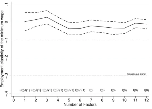
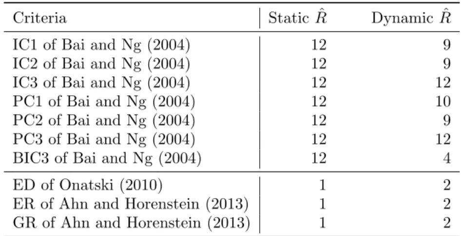
static model hold. In the case of the dynamic bias-corrected IFE estimator (Moon and Weidner, 2017) in column (4), it does depend on the number of factors used. Table A3 in the Appendix shows the suggested number of factors according to the various selection criteria available in the literature. We use ten factors as our baseline result as a) the tests suggest there should be at least nine factors, b) Moon and Weidner (2015) show that it is better to include too many factors than too few and c) the models with nine or fewer factors do not lead to stationary residuals. Figure A2 in the Appendix shows that this choice is of some importance. Up to nine factors, the dynamic IFE estimator predicts employment elasticities around -0.12, in line with the 2FE results. However, these estimates are not statistically significant (at 5%) and lead to non-stationary residuals.
The other SH-robust estimators are more unanimous, pointing to a complete lack of disemployment effects regardless of the method chosen. I.e. the pooled CS-ARDL (5) estimate is not distinguishable from zero. This does not change when moving to the CS-DL approach (6, see Section IV), nor when allowing for heterogeneous coefficients in the mean group CS-DL model (7).31
The statistics for these dynamic models are more encouraging than those for the static models although due to the uniform lag structure across models the improvement is limited. The 2FE model (1) still produce non-stationary residuals, though with limited serial cor-relation. The first difference (2), AH (3), IFE (4) and cross-sectionally augmented pooled ARDL model lead to stationary residuals, with mixed serial correlation evidence. The CS-DL models (6, 7) result in non-stationary, serially correlated residuals.
VI. Minimum Wages and Politics
There is a clear divide between the traditional estimators (TFE, 2FE) and the spatial heterogeneity robust estimators (CCEP/IFE), especially in the static models. Hitherto, the discussion of this difference has been purely statistical. Allegretto, Dube and Reich (2010) point out that adding state-specific trends or Census division specific time dummies
already leads to estimates close to zero. Dube, Lester and Reich (2010) take it one step further and add cross border county pair specific time dummies to limit the comparison to a very local level and find the same. The MFS models we illustrated and estimated in the previous sections are more general and do not impose a strong structure on the spatial heterogeneity.
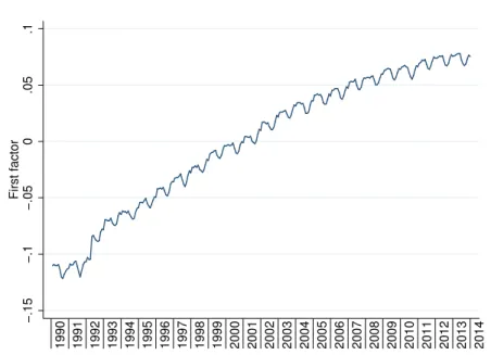
The advantage of this approach is that we can get a clearer view on the pattern of the SH present in the data by investigating the estimated factors and their loadings. Like Totty (2015), we find that the first factor closely resembles a seasonally adjusted time trend (Figure 4).32 This would explain why the state-specific time trends model leads to similar results as the SH robust estimators. Likewise, the factor loadings for this time trend are very similar within census divisions, explaining the results of the census division-specific time dummies approach (Figure 5). However, an economic interpretation is still missing. That is, what is the source of this spatial heterogeneity and why does it affect the minimum wage estimates?
One promising interpretation of this ‘spatial heterogeneity’ is that it reflects the shifting political climate in the US. Recent efforts in the field of political science have led to the development of new ‘ideal point’ measures, which position individual legislators on an axis ranging from liberal to conservative. In particular, Shor and McCarty (2011) have estimated ideal points that are consistent across space (US states) and time by combining roll-call data (who votes with whom) with answers to the National Political Awareness Test. These nation-wide survey responses serve as a bridge between state legislatures, allowing for a meaningful comparison between e.g. a Texas Democrat and a New York Republican (Bjørnskov and Potrafke (2013), Battista, Peress and Richman (2012)).
These individual ideal points can be combined to state-level indicators of political sen-timent by taking the median value per chamber. Figure 6 shows the evolution of political ideology of the state lower chambers (‘the House’). Positive values indicate a gradual shift towards more conservative notions. Negative values then refer to houses that have become
Figure 4. Evolution of the first factor (F1) over time. −.15 −.1 −.05 0 .05 .1 First factor 1990 1991 1992 1993 1994 1995 1996 1997 1998 1999 2000 2001 2002 2003 2004 2005 2006 2007 2008 2009 2010 2011 2012 2013 2014
more liberal. Two points are worth noting. First, there is great heterogeneity across the US: the south has become considerably more conservative, whereas the west and north-east have shifted left. Second, the map strongly resembles Figure 5, depicting the factor loadings of the MFS model. The average state factor loadings and the slope of the trend in political ideology are strongly correlated with a correlation coefficient of 0.41.
Could changes in political sentiment be the omitted variable that has afflicted minimum wage research since the 90s? From a theoretical perspective this would definitely make sense. On one hand, support for the minimum wage is starkly divided along political party lines.33 On the other hand, politics play a defining role in setting the balance between ease of doing business and health, safety, environmental and social regulations which in turn affect employment opportunities in the restaurant sector.34
In Table 4 we show what happens when we add this measure of political sentiment 33The Democratical Platform, detailing the stance of the Democratic party, has committed to introducing a $15
an hour minimum wage. Republicans unanimously voted against an increase in the federal minimum wage in 2013.
34We find some indications for this in the CNBC’s Top States for Business ranking. States which score more
conservative in our political measure are also rated more business friendly and have a lower cost of doing business (but also score worse on quality of life).
Figure 5. Loadings of the first factor (λ1) averaged by state. AZ CA CO ID IL IN IA KS ME MD MA MI MN MO MT NE NH NM NY ND OK OR SD UT VT WA WI WY AL AR CT DE FL GA KY LA MS NV NJ NC OH PA RI SC TN TX VA WV (1.01863,1.58429] (.372165,1.01863] (.054293,.372165] (−.004986,.054293] (−.231327,−.004986] (−.534183,−.231327] (−.824757,−.534183] (−1.1619,−.824757] [−1.61968,−1.1619]
Figure 6. Slopes of the trend in political ideology over time by state.
CA CO CT DE IA ME MD MA MT NV NH NJ NM NY ND OH OR PA RI SD UT VT WA WV WI WY AL AZ AR FL GA ID IL IN KS KY LA MI MN MS MO NC OK SC TN TX VA (.00282675,.01005418] (.00125674,.00282675] (.00035137,.00125674] (−.00043363,.00035137] (−.0009447,−.00043363] (−.00134164,−.0009447] (−.00237537,−.00134164] (−.0044496,−.00237537] [−.00904672,−.0044496]
Table 4—Employment - Politics included
Static Dynamic
(1) (2) (3) (4) (5) (6) (7)
CS-TFE 2FE IFE CCEP 2FE IFE ARDLP
Employment elasticity of the -0.088 -0.049 -0.003 -0.021 -0.054 -0.035 -0.034 minimum wage (-0.58) (-1.52) (-0.14) (-0.76) [-1.29] [-1.74] [-0.97] Median political 0.080∗∗ 0.041∗∗∗ 0.003 0.006 0.043∗∗∗ 0.006 0.013∗∗ ideology of house (2.35) (4.05) (0.68) (1.59) [4.09] [1.18] [2.51] N 217884 217884 168576 217884 217884 168576 217884
tstatistics in parentheses,z statistics in brackets, errors are clustered at the state level. Models (5)-(7) include lags 1, 2 and 6 for the dependent and independent variables (corresponding to one month, two months and two quarter delayed effects). Model (3) and (6) use 9 factors. All regressions include total private sector employment, population controls and monthly time dummies. The political measure is at times missing. The IFE models use a balanced panel, the others stay as close to the initial balanced panel as possible. The traditional estimates remain unchanged when using the slightly modified sample (unreported).
∗p <0.1,∗∗ p <0.05,∗∗∗p <0.01
to our main regressions. First and foremost, the large differences between the models disappear. From the simple time fixed effects model (column 1) to the dynamic cross-sectionally augmented ARDL model (7), all point to a lack of disemployment effects of the minimum wage once once shifts in political sentiment are controlled for. Second, the political measure coefficient is highly significant in the traditional estimators (columns 1, 2 and 5). These results provide an empirical backing for the omitted variable bias story, especially given that the political ideology measure is also correlated with the minimum wage (correlation coefficient: -0.18). Note that the political measure is not significant in all but one of the MFS models (3, 4, 6, but not 7).
VII. Robustness Checks
In this section we compare the performance of the MFS models and the politically aug-mented twoway fixed effects (POL2FE) model to that of the traditional estimators in various scenarios. A first concern is whether both types of models are able to detect sig-nificant effects if they are present. We test this by estimating the impact of minimum wage changes on earnings. If they fail to detect a positive relation, that would cast doubt
on the employment results. We find reasonable estimates in all cases. Second, we apply the main estimators to employment data from the accounting and finance sectors to see whether they find significant employment effects in these sectors unaffected by minimum wage policy. Here, the (traditional) twoway fixed effects model still points towards strong negative elasticities, whereas those of the richer models remain centered around zero. Fi-nally, reducing the sample to a balanced monthly panel might not be an innocuous change. We re-estimate the main models using first an unbalanced dataset and then the quarterly 1990-2006 panel used in Dube, Lester and Reich (2010). None of the conclusions change qualitatively, though it does raise some interesting questions.35
A. Earnings
In line with DLR and Totty (2015) we use wage data as a plausibility check of the estima-tors we employ. The idea is that if some detail of their working would lead to insignificant results regardless of the true effect, then we would also find insignificant earnings effects (the presence of which is not disputed in the literature). This is not as far fetched as it might sound. In a sample of 1000 panel units and four regressors, the CCEP estimator adds 1000∗(4 + 1) = 5000 regressors.
Based on data from Current Population Survey Merged Outgoing Rotation Groups (CPS-MORG) on individual hourly wages, we would expect a wage elasticity of 0.10, assuming minimum wage hikes only affect those below the new wage floor.36 However, the wage effect might not be confined to those directly affected by the legislative action (Grossman, 1983), hence higher coefficients are not necessarily problematic. Tables 5 and 6 show the wage elasticities for the various models. All estimators lead to significant positive elasticities, but the elasticities of the cross-sectional dependence robust estimators (columns 5 and 6 in Table 5, 5 in Table 6), ranging from 0.138-0.205 seem more credible than those produced by 35In Appendix A.A1 we also investigate how the 2FE and CCEP models react to different lag specifications. We
show that the results remain highly stable by illustrating the long run effects of the minimum wage on employment for an increasing number of lags of both the dependent and independent variable.
36Concretely, we take everyone in the MORG files that is employed in the restaurant sector and calculate the
percentage difference between their current wage and the next minimum wage as well as the relevant percentage change in the minimum wage. The average ratio of these two factors provides a rough estimate of the wage elasticity of the minimum wage, assuming those above the new minimum wage remain unaffected (their ratios are set to zero).
Table 5—Earnings - Static Models
(1) (2) (3) (4) (5) (6) (7)
POLS 2FE Trends CBCP IFE CCEP POL2FE
Wage 0.372∗∗∗ 0.226∗∗∗ 0.178∗∗∗ 0.177∗∗∗ 0.138∗∗∗ 0.190∗∗∗ 0.217∗∗∗
elasticity (6.86) (9.99) (6.71) (5.84) (10.24) (4.98) (10.40)
N 98880 98880 98880 43968 98880 98880 72628
CD 0.77 0.23 0.07 0.00 0.00 0.64 0.00
Order of Integration I(0)/I(1) I(0)/I(1) I(0)/I(1) I(0)/I(1) I(0) I(0)/I(1) n.a.
LM(1) 0.00 0.00 0.00 0.00 0.00 0.00 0.00
LM(2) 0.00 0.00 0.00 0.00 0.00 0.00 0.00
Notes: See Table 2. POL2FE refers to the twoway fixed effects model augmented with the political measure as control variable. As the political measure is sometimes missing, the panel in model (7) is not balanced and the stationarity tests cannot be applied.
∗p <0.1,∗∗p <0.05,∗∗∗p <0.01
Table 6—Earnings - Dynamic or Differenced Models
(1) (2) (3) (4) (5) (6)
POLS 2FE FD AH CCEP POL2FE
Long-run
wage 0.467∗∗∗ 0.257∗∗∗ 0.0863∗∗∗ 0.154∗∗∗ 0.205∗∗∗ 0.234∗∗∗
elasticity [7.20] [9.66] (19.35) (80.16) [4.37] [9.81]
N 96820 96820 97850 95790 96820 72628
CD 0.00 0.00 0.00 0.00 0.51 0.00
Order of Integration I(0) I(0)/I(1) I(0) I(0) I(0) n.a.
LM(1) 0.00 0.00 0.00 0.00 0.97 0.02
LM(2) 0.00 0.00 0.26 0.00 0.00 0.00
See Table 2 for a description of the diagnostic tests.F statistics in parentheses,zstatistics in brackets, errors are clustered at the state level. POL2FE refers to the twoway fixed effects model augmented with the political measure as control variable. Models (1), (2), (5) and (6) include lags 1 and 2 for the dependent and independent variables (corresponding to one and two quarter delayed effects). Model (3) estimates the entire model in first differences, Model (4) includes the same lags of the independent variable, but only the first lagged difference of restaurant employee earnings. All regressions include total private sector employment, population controls and quarterly time dummies. As the political measure is sometimes missing, the panel in model (6) is not balanced and the stationarity tests cannot be applied.
the standard regression models (0.226-0.467) (columns 1 and 2 in both tables). The twoway fixed effects model with political control variable (POL2FE) leads to wage elasticities nicely centered in the pack, suggesting that a 10% increase in the minimum wage raises average wages by 2.17% (2.34% in the dynamic setting).
B. Different Sectors
Above, we tested whether the various estimators find significant effects when they should. Now, we test whether they find such effects when they should not, by applying them to employment levels in the accounting (NAICS 5412) and finance (NAICS 52) sectors. Only 2-3% of employees in those industries earn up to 1.25 times the minimum wage (the corre-sponding number for the restaurant sector is 30%).37 Table 7 shows results for the main estimators. The spatial heterogeneity-robust estimators (columns 3 and 6) lead to insignifi-cant elasticity estimates in both sectors. The standard twoway-fixed effect model (columns 1 and 4) on the other hand still picks up strong negative employment effects, especially in the finance sector. The median wage of tellers, the lowest paid occupation in the finance sector, was $12.69 in 2015, almost twice the federal minimum wage at the time and more than $2 higher than the highest state minimum wage.38 As a result, the minimum wage does not ‘bite’, not even indirectly.39 Consequently, the strong negative effects suggested by the 2FE model are rather dubious. The trends (column 2) and politically augmented models (4) produce estimates approaching the -0.1 lower bound of the consensus band, but these are not statistically significant (at 5%).
C. Different Samples
Table 8 shows estimated employment elasticities using an unbalanced panel. We restrict the sample to counties with at least 120 observations to ensure the county-specific coeffi-37If we compare current earnings to the upcoming minimum wage, we get respectively 4% and 40%. Calculations
based on CPS-MORG data.
38Earnings data come from the Occupational Employment Statistics database.
39The minimum wage might still affect employees for whom the new wage floor is not binding (see Section VII.A),
but it is unlikely this effect ripples on that far into the wage distribution. Moreover, Autor, Manning and Smith (2016) call into question the existence of minimum wage spillovers, arguing that reporting errors might lead to spurious detection of wage effects on those above the wage floor.
Table 7—Employment - Different sectors
Sector Static Models Dynamic Models
(1) (2) (3) (4) (5) (6)
2FE Trends CCEP POL2FE 2FE CCEP
Accounting Long-run employment -0.183∗ -0.099∗ -0.017 -0.083 -0.171∗ -0.059 elasticity (-1.93) (-1.80) (-0.27) (-1.41) [-1.81] [-0.74] N 314784 314784 314784 231876 308226 308226 Finance Long-run employment -0.151∗∗∗ 0.028 0.004 -0.067∗ -0.216∗∗∗ 0.003 elasticity (-2.84) (1.03) (0.13) (-1.91) [-3.47] [0.06] N 586368 586368 586368 424416 574152 574152
t statistics in parentheses,z statistics in brackets, errors are clustered at the state level. POL2FE refers to the twoway fixed effects model augmented with the political measure as control variable. Models (5) and (6) include lags 1, 2 and 6 for the dependent and independent variables (corresponding to one month, two months and two quarter delayed effects). All regressions include total private sector employment, population controls and monthly time dummies.
∗p <0.1,∗∗ p <0.05,∗∗∗p <0.01
cients are still reliably estimated.40 We end up with 1866 counties (vs 1293 in the balanced
case and 3142 in the full sample). The static results remain qualitatively unchanged, with only twoway fixed effects leading to economically (but less statistically) significant em-ployment elasticities (column 1). Rather surprisingly, the model including state-specific trends (column 2) and the politically-augmented 2FE estimator (4) produce a statistically significant negative employment elasticity. However, the point estimate itself is still very small as it predicts a 10% increase in the minimum wage would only lead to respectively a 0.4% and 0.7% reduction in employment in the restaurant sector.
The dynamic models are similarly affected. On one hand, the twoway fixed effects elas-ticity is no longer statistically significant (column 5). On the other hand, the dynamic spatial heterogeneity-robust point estimate (column 6) becomes more negative, albeit in-significant. This does depend to some degree on the cut-off threshold. For example, when one restricts the sample to counties with at least 50 observations, the dynamic CCEP
Table 8—Employment - Unbalanced Panel
Static Models Dynamic Models
(1) (2) (3) (4) (5) (6)
2FE Trends CCEP POL2FE 2FE CCEP
Long-run
employment -0.158∗ -0.041∗∗ -0.049∗ -0.073∗∗ -0.132 -0.068 elasticity (-1.96) (-2.05) (-1.93) (-2.10) [-1.51] [-1.64]
N 496056 496056 496056 345981 475020 475020
See notes of Table 7.
estimate of the long run elasticity is -0.07, significant at 10% (p=0.07). While perhaps not sufficient to discredit the main conclusions, these results do indicate that reducing the sample to a balanced panel is not a trivial action, despite being standard in the literature. One potential explanation is that the minimum wage effect is highly heterogeneous across counties, suggesting there might be particular circumstances in which a higher wage floor does lead to job losses.
Table 9—Employment - Quarterly data
Static Models Dynamic Models
(1) (2) (3) (4) (5) (6)
2FE Trends CCEP POL2FE 2FE CCEP
Long-run
employment -0.166∗∗ -0.026 0.001 -0.052 -0.150∗ -0.050
elasticity (-2.28) (-1.14) (0.04) (-1.60) [-1.94] [-1.16]
N 98880 98880 98880 72628 96820 96820
See notes of 7.
Finally, Table 9 turns to the balanced quarterly data used in Totty (2015) and Dube, Lester and Reich (2010). We see the same trends as with the monthly data - increases in the minimum wage lead to reduced employment according to the fixed effects models (columns 1 and 5), but this effect disappears once one controls for cross sectional dependence, it be by adding state-specific trends (2), a measure of political sentiment (4) or the cross-sectional
averages (columns 3 and 6).
VIII. Conclusion
The impact of minimum wages on employment levels is hotly debated, with elasticity estimates very sensitive to the exact specification, especially with regards to how they deal with spatial heterogeneity and dynamics. We show that the most common approaches (leading to contradictory outcomes) can be nested in a general multifactor error structure framework. As a result, we can make use of specialised estimators which impose far fewer assumptions on the underlying model than traditional methods and are capable of detecting dynamic effects.
Once we control for cross sectional dependence and/or the potentially complicated dy-namics of minimum wage policy, we find no evidence to suggest it negatively affects em-ployment levels in the US. The only estimator that indicates strong disemem-ployment effects is the traditional twoway fixed effects estimator (time and county dummies). However, compared to the spatial heterogeneity-robust models, it performs worse at various statis-tical tests, produces less credible wage elasticity estimates and fares considerably worse in placebo tests, where it predicts strong disemployment effects in the finance and accounting sectors (which are unaffected by current minimum levels).
Additionally, we move beyond the purely statistical notion of spatial heterogeneity and show that the differences in the literature melt away once you control for (differential) shifts in political sentiment across the US. Politics affect both the level of the minimum wage and the economic and regulatory conditions of restaurants and fastfood joints. Failing to control for heterogeneous changes in ideology hence biases the estimates of the employment elasticity of the minimum wage. We find that both traditional and spatial heterogeneity robust estimators suggest there are no disemployment effects once a measure of political ideology is added to the regressions.
As a result, we conclude that given current data and modeling techniques, it is more likely that minimum wages do not adversely affect employment opportunities. There are two major caveats. First, the impact of a large minimum wage shock (e.g. the Living
Wage Adjustment, from $7.25 to $15) might be very different from the moderate changes observed so far. Second, the estimated employment elasticities of the richer models were noticeably more negative in the unbalanced panel than in the balanced case, indicating the impact might not be homogeneous across the various states. In turn, this suggests the minimum wage might lead to job losses in certain environments - further research is required to determine what they are.
REFERENCES
Abadie, Alberto, Alexis Diamond, and Jens Hainmueller.2010. “Synthetic Control Methods for Comparative Case Studies: Estimating the Effect of Californias Tobacco Control Program.”Journal of the American Statistical Association, 105(490): 493–505. Addison, John T., McKinley L. Blackburn, and Chad D. Cotti. 2015. “On the
robustness of minimum wage effects: geographically-disparate trends and job growth equations.”IZA Journal of Labor Economics, 4(1): 24.
Allegretto, Sylvia, Arindrajit Dube, and Michael Reich. 2010. “Do Minimum Wages Really Reduce Teen Employment? Accounting for Heterogeneity and Selectiv-ity in State Panel Data.” Institute of Industrial Relations, UC Berkeley Institute for Research on Labor and Employment, Working Paper Series qt7jq2q3j8.
Arellano, Manuel, and Stephen Bond. 1991. “Some Tests of Specification for Panel Data: Monte Carlo Evidence and an Application to Employment Equations.”Review of Economic Studies, 58(2): 277–297.
Autor, David H., Alan Manning, and Christopher L. Smith.2016. “The Contribu-tion of the Minimum Wage to US Wage Inequality over Three Decades: A Reassessment.”
American Economic Journal: Applied Economics, 8(1): 58–99.
Bai, Jushan. 2009. “Panel Data Models With Interactive Fixed Effects.”Econometrica, 77(4): 1229–1279.
Bai, Jushan, and Serena Ng. 2002. “Determining the Number of Factors in Approxi-mate Factor Models.”Econometrica, 70(1): 191–221.
Baker, Michael, Dwayne Benjamin, and Shuchita Stanger. 1999. “The Highs and Lows of the Minimum Wage Effect: A Time-Series Cross-Section Study of the Canadian Law.”Journal of Labor Economics, 17(2): 318–50.
Battista, James C., Michael Peress, and Jesse Richman. 2012. “Common-Space Ideal Points, Committee Assignments, and Financial Interests in the State Legislatures.”
State Politics & Policy Quarterly, 13(1): 70–87.
Bjørnskov, Christian, and Niklas Potrafke.2013. “The size and scope of government in the US states: Does party ideology matter?” International Tax and Public Finance, 20(4): 687–714.
Born, Benjamin, and Jrg Breitung. 2016. “Testing for Serial Correlation in Fixed-Effects Panel Data Models.”Econometric Reviews, 35(7): 1290–1316.
Breitung, Jrg. 1999. “The local power of some unit root tests for panel data.” Hum-boldt University of Berlin, Interdisciplinary Research Project 373: Quantification and Simulation of Economic Processes SFB 373 Discussion Papers 1999,69.
Brown, Charles. 1999. “Minimum wages, employment, and the distribution of income.” InHandbook of Labor Economics. Vol. 3, Part B. 1 ed., , ed. O. Ashenfelter and D. Card, Chapter 32, 2101–2163. Elsevier.
Brown, Charles, Curtis Gilroy, and Andrew Kohen. 1982. “The Effect of The Minimum Wage on Employment and Unemployment.”Journal of Economic Literature, 20(2): 487–528.
Burkhauser, Richard V., Kenneth A. Couch, and David C. Wittenburg. 2000. “A Reassessment of the New Economics of the Minimum Wage Literature with Monthly Data from the Current Population Survey.”Journal of Labor Economics, 18(4): 653–680.