SCUOLA DI DOTTORATO
Dottorato in Ingegneria Informatica e dei Sistemi – XXIV ciclo
Tesi di Dottorato
Speaker and Language
Recognition Techniques
Sandro Cumani
Tutore Coordinatore del corso di dottorato
l’inizio della loro opera e ora quanto avranno in progetto di fare non sarà loro possibile. Scendiamo dunque e confondiamo la loro lingua, perché non comprendano più l’uno la lingua dell’altro”.
Bibbia, Libro della Genesi 11, 1-9
Poi disse a me: “Elli stessi s’accusa; questi è Nembrotto per lo cui mal coto pur un linguaggio nel mondo non s’usa.
Lasciànlo stare e non parliamo a vòto; ché così è a lui ciascun linguaggio come ’l suo ad altrui, ch’a nullo è noto”.
Dante Alighieri, La Divina Commedia -Inferno: C. XXXI
Oh freddled gruntbuggly thy micturations are to me
As plurdled gabbleblotchits on a lurgid bee. Groop I implore thee, my foonting
turlingdromes.
And hooptiously drangle me with crinkly bindlewurdles,
Or I will rend thee in the gobberwarts with my blurglecruncheon, see if I don’t!
Prostetnic Vogon Jeltz, Douglas Adams, The Hitchiker’s Guide to the Galaxy
In this work we give an overview of different state–of–the–art speaker and language recognition systems. We analyze some techniques to extract and model features from the acoustic signal and to model the speech content by means of phonetic decoding. We then present state–of–the–art generative systems based on latent variable models and discriminative techniques based on Support Vector Machines.
We also present the author’s contributions to the field. These contributions cover the different topics presented in this work. First we propose an improve-ment to Neural Network training for speech decoding which is based on the use of General Purpose Graphic Processing Units computational framework. We also propose adaptations of latent variable models developed for speaker recognition to the field of language identification. A novel technique which enhances the gener-ation of low–dimensional utterance representgener-ations for speaker verificgener-ation is also presented. Finally, we give a detailed analysis of different training algorithms for SVM–based speaker verification and we propose a novel discriminative framework for speaker verification, the Pairwise SVM approach, which allows for fast utterance testing and allows to achieve very good recognition performance.
I would like to thank my parents, to whom I dedicate this work.
I would also like to thank professor Pietro Laface for his support during these last three years, and all the people I had the opportunity to work with:
• The people from Brno University of Technology, in particular Oldřich Plchot, Ondřej Glembek, Pavel Matějka, Lukáš Burget and Mehdi Soufifar, with whom I had the pleasure to collaborate sharing many interesting thoughts, ideas and great moments, Honza Cernocký, for hosting me twice at BUT, and all the other people from Brno who made me have a great and profitable time there. • The guys from Agnition, Niko Brümmer and Edward de Villiers, for all the discussions about generative and discriminative models and many memorable moments in Brno,
• All the other people who participated to the Bosaris workshop.
• The people from Loquendo, in particular Daniele Colibro and Claudio Vair, for the profitable collaboration in the last three years.
• My former collegues, Stefano Scanzio and Fabio Castaldo, with whom I had the opportunity to profitably work.
• All the people who I had the pleasure to interact with during workshops and conferences.
Summary iv
Acknowledgements v
1 Introduction 1
1.1 Speaker Recognition . . . 1
1.2 Language Recognition . . . 2
2 Modeling the acoustic signal 5 2.1 Acoustic Features . . . 5
2.1.1 Sampling, quantization and filtering . . . 5
2.1.2 Mel–Frequency Cepstral Coefficients . . . 7
2.1.3 Shifted Delta Coefficients. . . 9
2.2 Gaussian Mixture Models . . . 9
2.2.1 Gaussian Mixture Model . . . 9
2.2.2 Maximum likelihood estimate of a GMM . . . 11
2.3 Hidden Markov Models . . . 12
2.3.1 Topological structure . . . 12
2.3.2 Probabilistic structure . . . 13
2.3.3 Forward-Backward algorithm . . . 15
2.3.4 Viterbi algorithm . . . 16
2.3.5 Training . . . 17
2.4 Artificial Neural Networks . . . 18
2.4.1 Structure . . . 18
2.4.2 Feed–forward Neural Network and Perceptron . . . 19
2.4.3 Training . . . 20
2.4.4 ANN–HMM . . . 21
2.5 Phonotactic features . . . 24
2.5.1 Bags ofn-grams features for language identification . . . 25
2.5.2 Phonetic decoders. . . 28
3 Latent variable models for speaker and language recognition 35
3.1 Speaker verification problem . . . 35
3.2 Universal Background Models and GMMs . . . 36
3.3 Factor analysis models . . . 37
3.3.1 Statistics and likelihoods . . . 38
3.3.2 MAP adaptation . . . 40
3.3.3 Eigenvoice models. . . 41
3.3.4 Eigenchannels . . . 41
3.3.5 Joint factor analysis of speaker and channel . . . 42
3.4 Front–end JFA . . . 42
3.5 I–vectors . . . 43
3.5.1 I–vector posterior distribution . . . 44
3.5.2 Training the T matrix . . . 45
3.5.3 Speeding up the i–vector extraction . . . 46
3.6 Probabilistic Linear Discriminant Analysis . . . 53
3.6.1 Two covariance model . . . 55
3.6.2 Speaker verification likelihood . . . 56
3.6.3 PLDA . . . 57
3.6.4 Training the PLDA hyperparameters . . . 58
4 Discriminative Training and Support Vector Machines 61 4.1 Support Vector Machines and Logistic Regression . . . 61
4.1.1 Support Vector Machines. . . 61
4.1.2 Logistic Regression . . . 69
4.1.3 Regularized LR and SVM . . . 71
4.1.4 Multiclass SVM and LR for language recognition . . . 72
4.1.5 Multiclass Score Backprojection . . . 73
4.2 SVM–based language identification . . . 74
4.2.1 GSV–SVM and pushed–GMM . . . 75 4.2.2 Language factors . . . 76 4.2.3 Acoustic i–vectors . . . 77 4.2.4 Phonetic models . . . 78 4.3 Large–scale SVM algorithms . . . 79 4.3.1 Dual solvers . . . 80 4.3.2 Primal solvers . . . 82
5 SVM–based Speaker Recognition 87 5.1 GMM–SVM . . . 87
5.2.3 Pairwise SVM as likelihood approximation . . . 91
5.2.4 Polynomial Feature Mapping . . . 92
5.2.5 Fast scoring . . . 94
6 Experimental Results 97 6.1 GPU–based ANN training . . . 97
6.2 Language Identification . . . 99
6.2.1 Language Factors . . . 100
6.2.2 Phonotactic i–vectors . . . 101
6.3 Large–scale linear SVM training . . . 103
6.3.1 SVM algorithms implementation . . . 103
6.3.2 Algorithms for language recognition . . . 104
6.3.3 Algorithms for speaker recognition . . . 105
6.3.4 Language Recognition task results. . . 106
6.4 Pairwise SVM . . . 110
6.4.1 Pairwise SVM and PLDA . . . 110
6.4.2 Gender Independent PSVM . . . 112
6.4.3 Performance on non–NIST datasets . . . 114
6.4.4 Training the PSVM system . . . 116
6.5 I–vector extraction . . . 118
7 Conclusions 121 Bibliography 123 A Expectation–Maximization and HMM algorithms 133 A.1 The EM algorithm . . . 133
A.2 The Forward–Backward algorithm . . . 135
A.3 The Viterbi algorithm . . . 138
2.1 Timing profiles for MLP training using CUDA . . . 33
6.1 Training time for different ANN training algorithms . . . 99
6.2 ANN speed–up for different datasets . . . 99
6.3 Min DCF and (%EER) for the core closed set tests in LRE07 . . . . 102
6.4 Cavg×100 for different systems on NIST LRE09 . . . 102
6.5 Cavg×100 for different systems on NIST LRE09 with HDA. . . 103
6.6 Phonetic system: asymptotic valuesCavg and EER . . . 108
6.7 Phonetic system: time required to achieve 1% SVMLight C avg accuracy 108 6.8 Pushed–GMM: Cavg and EER for different training algorithms . . . . 110
6.9 PSVM and GPLDA on NIST 2010 SRE . . . 111
6.10 Improved PSVM and GPLDA on NIST 2010 SRE . . . 112
6.11 GI PSVM results on NIST SRE 2008 . . . 114
6.12 GI PSVM results on NIST SRE 2010 . . . 114
6.13 EER and DCF for different systems on different datasets . . . 115
6.14 SRE 2010 female tel–tel performance for BMRM and Pegasos . . . . 118
2.1 The A and µlaws . . . 6
2.2 Gaussian Mixture Model . . . 10
2.3 Left–to–right (Bakis) model . . . 13
2.4 Topological structure of a Multi–Layer Perceptron net . . . 19
2.5 Example of a HMM used in combination with a MLP . . . 22
4.1 Maximum margin hyperplane . . . 63
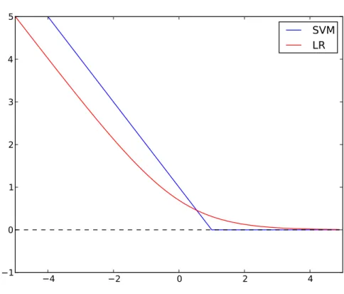
4.2 LR and SVM loss functions . . . 72
6.1 CUDA matrix–matrix multiplication . . . 98
6.2 MinDCF for different language factor subspaces . . . 101
6.3 Phonetic system: Cavg as a function of the training time . . . 109
6.4 EER and DCF vs subspace dimensionality for a GPLDA system . . . 113
6.5 SRE-10 DCF of Pegasos bunch sizes. . . 116
6.6 DCF10 and DCF08 with respect to training time for primal solvers . 117 A.1 Hiiden Markov Model . . . 135
Introduction
The growth of possible applications and the increase of computational power of processors has produced in the last years an increasing interest of both scientific community, industries and governments in automatic systems able to extract signif-icant information from spoken utterances. Research has developed on three main branches, namely speech, speaker and language recognition.
Speech recognition is involved with the creation of automatic transcriptions of speech, whose applications include device control through spoken commands or vir-tual typing.
Speaker recognition can be summarized as the creation of automatic systems which are able to answer questions regarding the identity of the person who is talking. Among speaker recognition applications we can cite authentication procedures, au-dio indexing, forensic activities.
Language recognition deals with identification of the language (e.g. English, Italian) used in a given utterance. This field includes applications in multilingual answering systems or as front–end for language–dependent speech recognizers.
The goal of this work is to present the author’s contributions to speaker verifi-cation and language recognition and, at the same time, offer an overview of state– of–the–art technologies for these fields.
1.1
Speaker Recognition
The goal of speaker recognition systems is to automatically make inferences about the identity of the speaker of a test utterance. Two main branches belong to speaker recognition, namely speaker identification and speaker verification.
Speaker identification can be described as a multiclass classification problem. Given a test utterance, we want to identify which, among a set of enrollment speak-ers, is the speaker of that utterance. The assumption of whether the test speaker
belongs or not to the enrollment set gives places to two different classification prob-lems, closed–set speaker identification and open–set speaker identification, the latter being more difficult.
Speaker verification requires a system to answer whether a test utterance belongs to a given speaker, or, equivalently, whether a set of recordings (e.g. one enrollment and one test segment) belong to the same speaker. While these two formulations are very similar, they correspond to two completely different discriminative speaker verification approaches.
1.2
Language Recognition
Similar to speaker identification, language recognition can be described as a multi-class multi-classification problem where the goal is to multi-classify an utterance according to its language. Again we can have both open–set and closed–set problems, depending on whether the test utterance is known to belong to given set of languages.
In this work we focus on the speaker verification problem and on closed–set language identification. These tasks are characterized by similar problems and share some modeling tools such as Gaussian Mixture Models, Factor Analysis or Support Vector Machines. The systems described in this work are characterized by a set of common modules, namely feature extraction, creation of models (e.g. speaker or language models, background models), test utterance scoring, normalization and calibration of scores.
This work details the contributions of the author to the state–of–the–art, and at the same time provides an overview of different language and speaker recognition technologies related to the first three modules. While score normalization and score calibration play an important role in real applications, they fall out of the scope of this work. References and details about score normalization techniques can be found in [1, 2, 3, 4,5], while [6] is an interesting treatise about calibration.
The outline of this work is the following.
• Chapter2describes the feature extraction process both for speaker recognition and language recognition systems and details some basic feature modeling techniques such as Gaussian Mixture Models, Hidden Markov Models and Neural Networks.
• Chapter 3 describes generative techniques for speaker recognition based on latent variable models.
Vector Machines (SVM) are introduced and applied to language identification problems.
• Chapter5 presents two frameworks for SVM–based speaker verification. • Experimental results regarding the author’s contributions to the state–of–the–
art are presented in Chapter 6. • Conclusions are drawn in Chapter 7.
Modeling the acoustic signal
In order to perform automatic speech recognition it is necessary to build mathe-matical models of the acoustic signal which can be used by a machine. In this chapter we analyze different techniques to transform the acoustic signal into a set of features which can be used to model the acoustic characteristics of speakers and lan-guages. The feature extraction techniques presented in this chapter form a common front–end to many different speaker and language recognition systems.
2.1
Acoustic Features
The first section of this chapter is devoted to acoustic feature extraction, i.e. to the steps which allow transforming an analog signal into a discrete set of features suited for speaker and language recognition systems.
2.1.1
Sampling, quantization and filtering
The first step in audio analysis consists in the transformation of the analog acoustic signal into a discrete version that can be processed by a machine. This representation is obtained by sampling and quantization of the acoustic analog signal.
Time–domain sampling corresponds to a multiplication of the input signal by a sequence of impulses Pkδ(t−kts) where ts is the sampling interval. Formally
ys(k) =
X
k
[y(kts)δ(t−kts)] (2.1)
where y(t) is the input signal and ys(k) is the sampled signal. This is equivalent,
in the frequency domain, to the convolution of a sequence of impulses with the spectrum of the analog signal, which gives
Ys(ω) = 1 ts X k Y ω+ 2πk ts ! (2.2)
where Y(ω) is the Fourier transform of y(t) and Ys(ω) is the Fourier transform of ys(t). In general the signal cannot be completely reconstructed due to the
over-lapping of replicas of the original spectrum (aliasing). However, since the human apparatus is sensitive only to frequencies lower than 4 kHz, it follows from Nyquist theorem that a sufficient sampling frequency for a speech signal corresponds to 8 kHz.
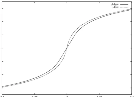
Quantization maps continuous values to discrete ones, thus it is always a lossy process. The simplest way to perform quantization consists in uniformly dividing the input range and assigning to each value the index of the corresponding interval (linear quantization). With this method, the quantization error corresponds to one least significant bit and, more important, its absolute value is constant for any given input value. The amplitude distribution of the acoustic signal signal is highly non– linear. To cope with this problem, a logarithmic quantization is usually performed, that is the logarithm of the acoustic signal is linearly quantized. In this way, the relative quantization error becomes constant. Since the logarithmic function is not defined in zero, slightly different functions are used in practice, as the µ–law (used in American communication nets) or the A–law (used in European communication nets) [7]. For telephone speech usually values are represented on 8 bits. In practice,
-0.6 -0.4 -0.2 0 0.2 0.4 0.6 -0.1 -0.05 0 0.05 0.1 A-law u-law
Figure 2.1: The A and µlaws
logarithmic quantization is done by performing linear quantization using a greater number of bits and then applying one of the laws in Figure2.1to map them to 8 bits.
Finally, in order to make the signal spectrum flatter in the given frequency band, the discrete samples are filtered by a first order pre–emphasis filter with transfer function
H(z) = 1−az−1 (2.3)
which is equivalent, in the time domain, to ˆ
Y(k) =Y(k)−aY(k−1) (2.4)
where a is a constant. Usually a= 0.95 in real applications.
2.1.2
Mel–Frequency Cepstral Coefficients
A standard representation of acoustic signal used in state–of–the–art speaker recog-nition systems is given by Mel–Frequency Cepstral Coefficients (MFCC) [8,7], which provide a short–term representation of the power spectrum of the acoustic signal.
Since the acoustic signal can be considered stationary over time spans of the order of milliseconds, it can be split into frames (usually covering about 10 ms) which group together a set of samples. This operation can be described as
Xt(n) = ˆY(Mat+n) 0≤n ≤Na−1, 0≤t≤T −1 (2.5)
where Na is the grouping window size, Ma is the size of the shift (i.e. Ma =Na/2), T is the duration in frames of the signal (the number of frames we split the signal into).
Since the grouping in frames results in a distortion of the spectrum of the samples of each frame (Gibbs phenomenon), the influence of samples near the borders of a frame is reduced, usually by means of a Hamming window
ˆ Xt(n) =Xt(n)W(n) 0≤n≤Na−1, 0≤t ≤T −1 (2.6) where W(n) = ( c+ (1−c) cos πn N−1 − π 2 if 0≤n ≤N −1 0 otherwise (2.7)
In real applications a typical value for c is c= 0.54. While this approach allows to
obtain a better approximation of the original signal spectrum, it penalizes informa-tion contained in border samples of each frame. To compensate for this problem the window is shifted only by half its size. In this way, samples which are on the border of a frame are in the middle of either the previous or the next one.
The following step consists in performing the Fourier transform over the data of each frame Xf(j) = F ˆ Xt(n) (j) 0≤n, j ≤Na−1, 0≤t, f ≤T −1 (2.8)
This spectrum is processed using filters which emulate the human apparatus. A simple but effective model represents the human auditory system as a filter bank. The acoustic signal spectrum is therefore divided according to frequency bands. We consider a filter bank where bands are constructed according to the Mel scale [7]. For each band the energy of corresponding samples is evaluated as
Ei(f) = Hi X
j=Li
|Xf(j)|2 1≤i≤Nf (2.9)
whereEi(f) is the energy of thei–th band,Liis the lower bound of the corresponding
band andHi is its higher bound. Nf is the number of bands (e.g. usuallyNf = 13).
Finally, MFCCs are computed as the Discrete Cosine Transform of the logarithm of the energy parameters Ei(f)
Ci(k) = Nf X j=1 log(Ej(k)) cos " i j− 1 2 π Nf # 0≤i≤Nf −1 (2.10)
whereCi(k) denotes thei–th MFCC for frame k [7].
The total energy of the frame can be evaluated as
E(k) =
Nf X
j=1
Ej(k) (2.11)
Since the energy information contained in C0(k) is the same information given by E(k), usually the cepstral parameter C0(k) is discarded. Moreover, it can be shown
that cepstral parameters have decreasing variance as their indices grow, so high index parameters can be discarded, since they convey less information. Usually, the number pof cepstral parameters used ranges from p= 12 top= 24.
In order to better model the acoustic signal, generally MFCCs are combined with their differential counterparts (depstral parameters). These parameters are evalu-ated through an approximation of the temporal derivative of MFCCs, for example using a polynomial expression over a given number of consecutive frames such as
∆ ¯Ci(k) =G N
X
j=−N
jC¯i(k−j) 1≤i≤p (2.12)
whereGis a gain used in order to have a similar variance between the set of cepstral and the one of depstral parameters and N is half the size of the window used to approximate the derivative. In the same way it is also possible to evaluate the differential energy as ∆E(k) = N X j=−N jE(k−j) (2.13)
State–of–the–art systems usually also compute second–order derivatives of cepstral coefficients in a similar way. The set of cepstral parameters and their first and second order derivatives becomes then observed feature vector
Ot = {C¯1(t), . . . ,C¯p(t),∆ ¯C1(t), . . . ,∆ ¯Cp(t),∆∆ ¯C1(t), . . . ,∆∆ ¯Cp(t),
E(t),∆E(t),∆∆E(t)} (2.14)
To make systems more robust, often post–processing techniques are applied to MFCCs, as for example feature warping [9]. These techniques try to compensate short–term distortions due to noise and channel mismatches.
2.1.3
Shifted Delta Coefficients
While MFCCs allow very good results in speaker recognition, language identification model performance can be improved by using Shifted Delta Cepstral (SDC) [10,11]. SDCs allow including additional temporal information with respect to standard MFCCs and have been motivated by the success of phonotactic approaches, whose features are based on longer temporal time spans than MFCCs (Section2.5). SDCs are specified by 4 parameters, N, d, P and k, where N is the number of cepstral
coefficients for each frame, d is the size of the delay for delta computations,k is the number of blocks whose delta coefficients are concatenated in the final feature vectors and P is the time shift between consecutive blocks [10, 11]. The SDC coefficients
∆cj(i, t) at time t are computes as
∆cj(i, t) = ¯Cj(t+iP +d)−C¯j(t+iP −d) (2.15)
where ¯Cj(t) is the j–th MFCC coefficient for time t.
2.2
Gaussian Mixture Models
The acoustic signal can be interpreted as a piecewise stationary stochastic process. Acoustic features can be interpreted as realizations (observations) of some random variables. An effective technique to model the underlying distribution of such vari-ables is given by Gaussian Mixture Models (GMMs) [12].
2.2.1
Gaussian Mixture Model
Given a (multivariate) random variableX with its own probability density function (pdf) f(x), a Gaussian Mixture Model (GMM) can be used to approximate an estimate of f(x) from a set Xs = {x1, . . . , xn} of samples of X. A GMM [12] is
a weighted sum (mixture) of a set of m (multivariate) normal distributions of the form P(x|M) = m X i=1 wiN(x|µi,Σi) (2.16)
where P(x|M) is the probability of x given the GMM model M and ci are the
mixture weights. N(x|µi,Σi) is a normal pdf with mean µi and covariance matrix
Σi Ni(x|µi,Σi) = 1 (2π)D/2 |Σi|1/2 exp −12(x−µi)TΣ−i 1(x−µi) (2.17) where D denotes the dimensionality of input space. The weights wi are also called
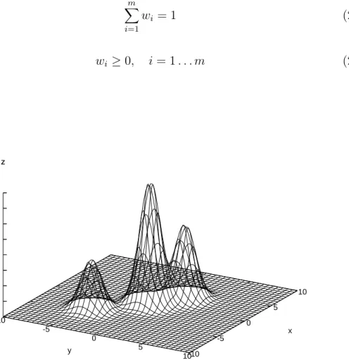
mixing coefficients and are constrained by
m X i=1 wi = 1 (2.18) wi ≥0, i= 1. . . m (2.19) -10 -5 0 5 10-10 -5 0 5 10 0 0.01 0.02 0.03 0.04 0.05 0.06 0.07 0.08 z y x z
An interesting formulation of a GMM can be given in terms of discrete latent variables [12]. Let Z = [z1, . . . , zm] be a m–dimensional random variable such that zi ∈ {0,1} and Pmi zi = 1, i.e. one single element of Z is equal to 1 while all the
others are equal to 0. Let the distribution of zk be defined in terms of the mixing
coefficients wi as
p(zk= 1) =wk (2.20)
that is, since only one term of Z is equal to one and the others are equal to zero,
p(Z) = Ym
i=1 wzi
i (2.21)
The realizations ofZ can be interpreted as representations of m mutually exclusive
states, of which only one is active. Assuming that, for each state, the conditional probability p(x|z) of random variableX given state zk = 1 is
p(x|zk = 1) =N(x|µk,Σk) (2.22)
the marginal probability of X can then be obtained by summing the joint distribu-tion p(x|z)p(z) over all values of Z
p(x) =X z p(z)p(x|z) = m X i=1 wiN(x|µi,Σi) (2.23)
which has the same form of our original Gaussian Mixture model (2.16).
The main advantage in using GMMs is their capability to accurately approximate any probability density function, given enough components in the mixture. However, we have to estimate GMMs parameters ϑ ={ci, µi,Σi} describing model M from a
sufficiently large set of samples of the random value. A possible approach consists in performing a Maximum–Likelihood (ML) estimate [13, 12], which looks for the solution of
ϑM L = arg max
ϑ P(Xs|ϑ) (2.24)
One of the advantages of representing a GMM as a latent variable model is that it allows for an easy derivation of a ML training procedure through the Expectation– Maximization algorithm (more details about the EM algorithm can be found in Appendix A.1).
2.2.2
Maximum likelihood estimate of a GMM
The Maximum Likelihood estimate of a GMM can be computed by means the Expectation–Maximization (EM) algorithm [12,14,15,16,13]. Letw0, µ0,Σ0denote
between the E and M steps as follows. During the E–step, for each observation xi
the posterior distributions of hidden variablesZi associated to observationxi, given
the current model parameters wc, µc,Σc, is computed as
p(zik = 1|xi, θc) =γik(θc) = wc kN(xi|µck,Σck) Pm j=1wcjN(xi|µcj,Σcj) (2.25) The parameters are updated in the M step to maximize the EM auxiliary func-tion Q(w, µ,Σ, wc, µc,Σc) = P
ip(zi|xi, wc, µc,Σc) logp(xi, zi|w, µ,Σ). The update
formulas are wk = Pn i=1γik(θc) Pn i=1 Pm j=1γij(θc) (2.26) µk = Pn i=1γik(θc)xi Pn i=1γik(θc) (2.27) Σk = Pn i=1γik(θc)(xi−µk)T(xi−µk) Pn i=1γik(θc) (2.28) A commonly used stopping criterion for the algorithm is the convergence of the likelihood P(X|w, µ,Σ).
Since estimating full covariance matrices is often difficult due to the scarcity of data and a increasing computational load, usually GMMs are estimated under the assumption that covariance matrices are diagonal. The loss in terms of modeling capabilities of the GMM is compensated by an increase in the number of components in the mixture [13].
2.3
Hidden Markov Models
Gaussian Mixture Models provide a compact and powerful representation of a set of acoustic features. However, temporal information is lost, since all frames are considered independent. A possible solution to account for temporal evolution of the acoustic signal consists in the use of Hidden Markov Models (HMM) [17,12].
A HMM is a finite state machine characterized by two stochastic processes. The first one is responsible for the discrete temporal evolution across the system states, while the second generates the observation samples which form the acoustic event. The first process cannot be directly observed (hidden), but can be estimated from the frame sequence generated by the model.
2.3.1
Topological structure
From a topological view, a HMM is a directed graphG(S, E) whereS ={S1, . . . , SN}
Markov model allows each state to reach any other state, in speaker and language recognition systems usually a simplified structure is adopted, which follows the tem-poral evolution of the acoustic event.
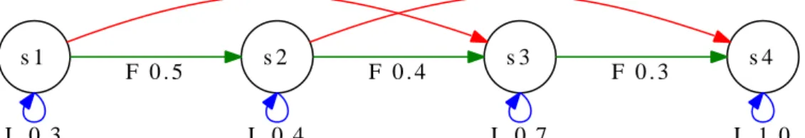
This simplified model, named Bakis linear model or left–to–right model [17], is characterized by a well established topological order of the nodes and presents only three kinds of edges: self–loop edges, forward edges (those ending in adjacent states) and skip edges (those ending in non adjacent states). Backward edges are not present, so the graph does not present any loop apart from self–loops. Each state identifies a stationary interval of the acoustic event, while the presence of self– loops allows to remain on the same state for longer periods, thus granting this model the capability to dynamically align the acoustic segment to the model. Moreover, this model imposes a minimal duration of the acoustic event, corresponding to the shortest path linking the first node to the final one.
s 1 L 0 . 3 s 2 F 0 . 5 s 3 S 0 . 2 L 0 . 4 F 0 . 4 s 4 S 0 . 2 L 0 . 7 F 0 . 3 L 1 . 0
Figure 2.3: Left–to–right (Bakis) model
2.3.2
Probabilistic structure
The evolution through the states of a HMM is controlled by a stochastic process described by transition probabilities. Given qt, the system state activated at time t, we can define π = (π1, . . . , πN) as the array of initial probabilities, that is the
probabilities of being in state Si at time t= 1
πi =P(q1 =Si) 1≤i≤N (2.29)
N
X
i=1
πi = 1 (2.30)
Transition probabilities are described by a matrix
whereaij =P(qt+1 =Sj|qt=Si) is the probability of reaching state Sj fromSi in a
single step. As such, the following properties hold
aij ≥0 ∀(i, j) (2.32)
N
X
j=1
aij = 1 ∀i (2.33)
In theory transition probabilities could also depend on the time t and on the observed sequenceX. However, a simplified approach considers the transition prob-abilities as a stationary, first order Markovian process, for which the following prop-erties hold
P(qt=Si|qt−1 =Sj, x1, . . . , xt−1) =P(qt=Si|qt−1 =Sj) (2.34)
and
P(qt=Si|qt+1 =Sj) =aij ∀t= 1. . . N −1 (2.35)
that is, transition probabilities do not depend neither on time nor on observed features.
Each state is associated to a stochastic function fi(xt) which represents the
probability of generating feature xt when the system is inSi. Usually it is assumed
that acoustic features are generated independently given the state, that is
P(xt|qt =Si, x1, . . . , xt−1) =P(xt|qt=Si) (2.36)
In many real systems the functions fi are, in fact, GMMs. An example of
applications of these systems is speech decoding, where the GMMs are used to model the distribution of acoustic features given the HMM state [7]. Often, in these models the state–dependent GMMs share mean and covariance values. In this case, eachfi(x) has the form
fi(x) = N
X
j=1
wijN(x|µj, Uj) 1≤i≤N (2.37)
where the mean vectorsµj and covariance matrices Uj do not depend on the state,
while the weights wij still do. This approach allows for a reduction in the number
of parameters with respect to a model where mean vectors and covariance matrices depend on the state.
In the following three sections we analyze the three main problems related to the use of HMMs [17], namely how to compute the probability of a set of observed features given the model parameters, how to evaluate the state sequence which best explains the observations (where “best” is defined according to a Maximum Likelihood criterion) and how to estimate the model parameters as to maximize the likelihood of some observations.
2.3.3
Forward-Backward algorithm
The first problem we address is how to evaluate the probability of a sequence of observed features O = {o1, . . . , oT} given the model M. This could, in theory, be
done by summing over all possible T–long sequences of states Q={q1, . . . , qT} the
joint probability of the sequence Q and of the observationsO P(O|M) =X
Q
P(O|Q, M)P(Q|M) (2.38)
Under the assumption of statistically independent observed features, this becomes
P(O|M) = X Q T Y t=1 P(ot|Q, M)P(Q|M) = X Q T Y t=1 P(ot|qt, M)P(Q|M) = X Q T Y t=1 fqt(ot)P(Q|M) (2.39)
where P(Q|M) can be evaluated as
P(Q|M) =πq1 TY−1
t=1
aqtqt+1 (2.40)
Assuming independent features is conceptually incorrect, since the acoustic signal presents a high degree of correlation between consecutive frames. However, this assumption is often used because it greatly simplifies the computations related to these kind of models. In the following we will assume feature independence. The approach of (2.39) is computationally unfeasible, since it requires a number of op-erations which grows exponentially with T (its complexity is OT NT [17]). The
Forward–Backward algorithm [17, 18] allows a much faster evaluation of P(O|M) (complexity O(T N2) [17]), exploiting that the probability of being in state S
i at
timet having observed the sequenceo1, . . . , otcan be evaluated from the probability
of being in each state Sj at timet−1.
Let αt(i) denote the forward probabilities of being in state Si at time t having
observed the sequence o1, . . . , ot and βt(i) denote the backward probabilities of
ob-serving, from time t+ 1 to T, the sequence ot+1. . . oT given that the system is in
state Si at time t, i.e.
αt(i) =P(qt=Si, o1, . . . , ot|M), α1(1) =f1(o1) (2.41) βt(i) =P(ot+1, . . . , oT|qt=Si, M), βT(f) = 1 (2.42)
where S1 is the initial state and Sf is the final state. The forward probabilities at
time t+ 1 can be computed from the forward probabilities at time t as αt+1(j) =
N
X
i=1
αt(i)aijfj(ot+1) (2.43)
while for the backward probabilities the following holds
βt(i) = N
X
j=1
βt+1(j)aijfj(ot+1) (2.44)
The computation of the forward and backward probabilities can then be done in
O(T N2). The quantity P(O|M) can be obtained from the forward and backward
probabilities as P(O|M) = N X j=1 αt0(j)βt0(j) (2.45)
wheret0 represents any frame, thus the overall complexity isO(T N2). More details
about the forward–backward algorithm are given in Appendix A.2.
2.3.4
Viterbi algorithm
The second problem involving HMMs consists in finding the sequence of statesQ=
{q1, . . . , qT} which best explains the observed features O ={o1, . . . , oT}. Different
criteria might be chosen to define optimality. In this context we assume that the best sequence refers to the sequence of states which is jointly most likely, that is the sequence S∗ defined as
S∗ = arg max
S P(Q=S, O|M) = arg maxS P(Q=S|O, M) (2.46)
A possible solution can be computed through the Viterbi algorithm [17, 18], which is equivalent to a minimum path search algorithm over the trellis associated to the HMM (for more details and the derivation of the algorithm see Appendix
A.3)
Assuming that the HMM has a single starting nodeS1, the algorithm evaluates,
for each time frame, the probability of the best path ending in state k at time t
(denoted asδt(k)) and keeps the pointerψt(k) to the node for which the probability
of reaching state k at time t is maximum. The algorithm proceeds as follows 1. initialize δ1(1) andψ1(i) as
δ1(1) = f1(o1) (2.47)
since the starting state has no parent node
2. iteratively evaluate the δ value of each node as t increases as
δt(i) = max
j (δt−1(j)aji)fi(ot) (2.49)
and update the corresponding backpointer ψt(i) using
ψt(i) = arg max
j (δt−1(j)aji) (2.50)
The best sequence ˆQ={qˆ1,qˆ2, . . . ,qˆT}can be evaluated by setting ˆqT =Sf and
following the backpointers up to the first frame ˆqt = Sψt+1(ˆqt+1). The probability of
the best path is δT(f), where f is the index of the final stateSf.
2.3.5
Training
Training a HMM consists in evaluating the model parameters θ = (A, B, π) with
A={aij}, B ={fi(x)} and π={π1, . . . πN} in order to maximize the likelihood of
an observed sequence given the model P(O|θ), this to adapt the model parameters so that they best describe the training data. Once again, this can be done by per-forming Maximum–Likelihood estimation through the Expectation–Maximization algorithm [17, 12].
In this section we give the re–estimation formulas for the model parameters at each iteration. The full derivation of these formulas can be found in Appendix A.4. Letθc represent the current estimate of the model parameters (which are
identi-fied by the superscript c) andαc
t(i),βtc(i) be the forward and backward probabilities
of stateSi at time trespectively, with α0(j) =πj and βT(j) = 1, computed through
the forward–backward algorithm using the current estimate of the model parame-ters. The new parameters can be evaluated as
aij = PT t=1αct−1(i)acijβtc(j) hP kwk,jc N(ot|µck,j,Σck,j) i PT t=1αct−1(i)βtc−1(i) (2.51) wi,j = PT t=1αct(j)βtc(j) PT t=1αct(j)βtc(j) wc i,jN(ot|µ c i,j,Σ c i,j) Pm k=1w c
i,kN(ot|µci,k,Σci,k)
(2.52) µi,j = PT t=1αct(j)βtc(j) wc i,jN(ot|µ c i,j,Σ c i,j) Pm k=1w c
i,kN(ot|µci,k,Σci,k)ot PT
t=1αct(j)βtc(j) wc
i,jN(ot|µci,j,Σci,j) Pm k=1w c i,kN(ot|µ c i,k,Σ c i,k) (2.53)
Σi,j =
PT
t=1αct(j)βtc(j) wc
i,jN(ot|µci,j,Σci,j) Pm k=1w c i,kN(ot|µ c i,k,Σ c i,k) (xt−µi,j)T(xt−µi,j) PT t=1αct(j)βtc(j) wc i,jN(ot|µ c i,j,Σ c i,j) Pm k=1w c
i,kN(ot|µci,k,Σci,k)
(2.54)
2.4
Artificial Neural Networks
Another set of models which have broad applications in speech technology are Arti-ficial Neural Networks. In particular, in the context of speech recognition ArtiArti-ficial Neural Networks are often used in combination with HMM to provide a fast and discriminative way to perform speech decoding [19].
2.4.1
Structure
An Artificial Neural Network [20] (ANN) is a directed graph G(I, N, O, E) where I denotes the set of input nodes, O denotes the set of output nodes, N is the set of internal nodes and E is the set of edges. Input nodes receive their inputs from outside the net, while output nodes expose values out of the net. Each non–input node has associated a set of parent nodes as described by the graph edges. An edge from node ni to node nj will be denoted as ξi,j, the set of input units of a given
node as S(i) and the set of output units of a given node as D(i).
Each unit of the net ni is characterized by an input value ni(t), an activation
value ai(t) and an output value oi(t). These values depend on the input pattern of
the net x. Each edge ξi,j has associated a weight wi,j (or, which is equivalent, each
unit has associated a set of weights, one for each of its input units).
The output value is evaluated as a function of the current activation value
oi(t) =Fi(ai(t)) (2.55)
while the new activation value is updated using a function of the current activation value and the inputs of the unit as
ai(t+ 1) =fi(ai(t), ni(t)) (2.56)
wherefi(x) is called activation function. The output functionFi(x) is usually either
the identity function Fi(x) = x, a threshold function or a stochastic function (e.g.
Gaussian). The activation function fi(x) usually is either a threshold function, a
semi–linear function (e.g. sigmoid, hyperbolic tangent) or a stochastic function (e.g. Gaussian).
Artificial Neural Networks are able to “learn” an association between input pat-terns and output patpat-terns by adjusting the weights of the net in such a way that
the net output corresponds to a given pattern when the net is fed a given input. Several types of network exist, the main differences lying in the topological struc-ture and in the learning algorithm used. Since in speech recognition we mostly deal with feed–forward networks usually derived from the Multi–Layer Perceptron, the following sections will focus on this kind of networks.
2.4.2
Feed–forward Neural Network and Perceptron
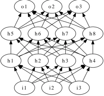
Feed–forward neural networks are characterized by the absence of cycles. The units are organized in layers (Figure 2.4)
i 1 h 3 h 4 h 1 h 2 i 2 i 3 h 7 h 8 h 5 h 6 o 1 o 2 o 3
Figure 2.4: Topological structure of a Multi–Layer Perceptron net
A very popular feed–forward network is the Multi–Layer Perceptron [20], which is characterized by the presence of one or more hidden layers between the input and the output layer. When used in speech recognition the activation functions are usually sigmoid functions. Sometimes output units have a soft–max activation function (Section 2.4.4).
Each unit evaluates its input value as
ni(t) =
X
j∈S(i)
wj,ioj(t) +bi (2.57)
where bi is a fixed bias. The output is evaluated as
with
f(x) = 1
1 +e−x (2.59)
The strength of the MLP consists in being able to approximate any kind of division surface given enough hidden nodes and enough hidden layers (i.e. two hidden layers [21]). Usually, the number of hidden layers is limited to 1 or 2.
2.4.3
Training
The training algorithm used with feed–forward networks goes under the name of backward propagation [22] and tries to minimize the classification error of the net-work. Let xp = (x1p, . . . , xN p) be an input pattern p of the net (which has N input
units), tp = (t1p, . . . , tM p) be the M target output values corresponding to xp and op = (o1p, . . . , oM p) the output values of the net given input pattern xp. The set of
output units will be denoted asO. The error function can be expressed as
E =X
p
E(p) (2.60)
where the errorE(p) for a given pattern pcan be expressed as the sum of the errors
ej(p) of each output unit nj
E(p) = X
j∈O
ej(p) (2.61)
The back-propagation algorithm minimizes the error function using gradient de-scent in the weights space. Weights are adjusted according to
∆wi,j =−k ∂E ∂wi,j =−kδj ∂nj ∂wi,j =−kδjoi (2.62) with δj = ∂E ∂oj ∂oj ∂nj (2.63) The update rule for the output layer weights is straightforward, since ∂E
∂oj depends only on the form ofE(p).
The back–propagation algorithm allows to update hidden layer weights by back– propagating (hence the name) the output layer error through the network. In par-ticular, in order to update weights for nodes in layer L we need to compute the values of δj for such nodes. The term ∂n∂ojj depends only on the node structure (i.e.
its activation function). For the error term ∂E
∂oj we make explicit its dependency on input values of layerL+ 1 as
∂E ∂oj = X i∈D(j) ∂E ∂ni ∂ni ∂oj ! (2.64)
Since ∂E
∂ni =δi and
∂ni
∂oj =wi,j we can rewrite the derivative of the error function as
∂E ∂oj
= X
i∈D(j)
(δiwi,j) (2.65)
Therefore, in order to computeδj for a layer in Lwe only need errorsδi of nodes
in layerL+1. The backpropagation consists then in a gradient descent optimization where the weights are updated according to
∆wti,j+1 =−ηt ∂E ∂wt i,j
=−ηtδjtoti (2.66)
wti,j+1 =wi,jt + ∆wi,jt+1 (2.67)
whereηtis the learning rate at time tand wi,jt is the value of weightwi,j at iteration t. In order to improve the convergence rate often a momentum term [20] is added, which also partially allows to avoid getting stuck in local minima. Let β denote the momentum coefficient. The update rule then becomes
∆wti,j+1 =−ηtδjtoti +β∆wi,jt (2.68)
wti,j+1 =wi,jt + ∆wi,jt+1 (2.69)
The back–propagation algorithm can be initialized using small random values as initial guess of the net weights.
2.4.4
ANN–HMM
An attractive alternative to GMM–based HMM is given by hybrid HMM–ANN models [19]. In these models an ANN is used in place of a GMM to estimate posterior probabilities of states given the observations. ANNs allow for a faster computation of posteriors than GMMs and are intrinsically discriminative. However, neural networks are designed to classify static patterns, which makes training more complex, and, moreover, require a large amount of training data. On the other hand, while GMMs are based on the assumption of statistical independence between consecutive frames, this is not the case of ANN–HMMs. In fact ANN–HMM models are often trained using a frame together with its left and right contexts [23].
Structure
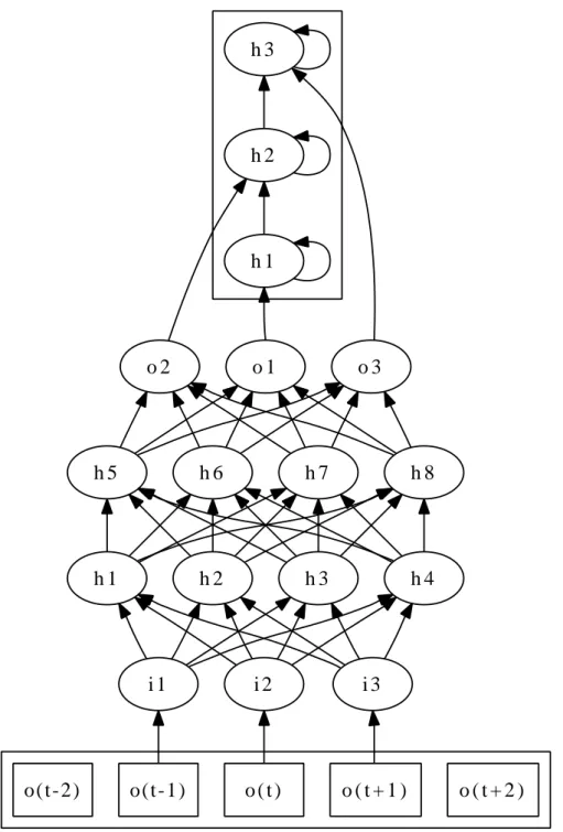
A classical topology for the ANN part of the model consists in a Multi–Layer Per-ceptron (MLP) where consecutive layers are fully connected (Figure 2.5).
In this case, the net is fed a frame together with its context and each node of the net is associated to a node of the HMM.
o(t-1) i 1 o(t-2) o ( t ) i 2 o ( t + 1 ) i 3 o ( t + 2 ) h 1 h 2 h 3 o 1 o 2 o 3 h 3 h 4 h 1 h 2 h 7 h 8 h 5 h 6
The output value of the net is the probability associated to the corresponding HMM node for the given frame (thus it has the same role of GMMs in GMM–based HMMs). Usually, input and hidden layers have sigmoidal activation functions.
Output units, instead, are often characterized by softmax activation functions, which allow to interpret the network outputs as posterior class probabilitiesP(ci|xt)
for class ci given the observed feature vector xt. The output of the networks are
computed as oi = eni P j∈Oenj (2.70) so that 0≤oi ≤1 ∀i∈O (2.71) and X i∈O oi = 1 (2.72)
The main disadvantage of these kind of models is the need to retrain the complete model when a new class is added. In speaker recognition, for example, where it is usual to add new speakers, this can pose some issues since training a neural network is a time consuming task.
Usually we are interested in the class–conditional probability of observed features
P(xt|ci). This can be evaluated resorting to the Bayes theorem as P(xt|ci) =
P(ci|xt)P(xt) P(ci)
(2.73) If we make the hypothesis of equiprobable distribution for P(xt) we have
P(xt|ci)∝
P(ci|xt) P(ci)
(2.74) This way, we can compute the posterior probability of an observed vector given a class up to a multiplicative factor. The prior probability can be taken into account by including it in the biases of the last layer as
bnewi =bi −logP(Ci) (2.75)
Training
The main problem when using hybrid ANN–HMM models lies in the training stage, since training an ANN would require to have fixed targets for each pattern, while in speech recognition this is not the case. The change of target values is due to the segmentation process used to label the given utterance (i.e., when using ANN–HMM models as phonetic recognizers, we need to identify phonemes corresponding to each
part of the sentence). Since manual segmentation is not feasible due to the high cost it would require, automatic segmentation is used, which, in turn, is not completely accurate but depends on the model used to perform it: the better the model, the better the segmentation. As we refine our ANN–HMM model, the segmentation itself usually changes, thus causing the change of target values (i.e. if we label a given segment with a different phoneme, then the ANN units corresponding to that phoneme would have one as target value; when we change the label, those units will have zero as target value). Training such a system requires an initial segmentation, often obtained by using other kind of models such as GMM–HMMs.
The procedure used to perform training can be described as 1. initialize the network with small random weights
2. load the actual segmentation (or the initial one if this is the first iteration) 3. train the model with several iterations of the back propagation algorithm in
order to obtain a model which approximates the targets given by the actual segmentation
4. compute the new segmentation using the current model
5. update the current segmentation by taking into account both the old and the new segmentation (e.g. the new segmentation target values can be evaluated as a weighted sum of the old target values and of those computed during the previous step)
6. repeat from 2.
Computing the actual segmentation can be done using the Viterbi algorithm and labeling the sentence with the symbols associated with the states of the best path of the Markov model [7].
2.5
Phonotactic features
Acoustic features are often directly used to create speaker and language models, as described in the next chapters. While acoustic models allow very good performance both for speaker and language verification, state–of–the–art systems often employ models based on higher level features which provide useful complementary infor-mation to acoustic models. In this section we will focus on the use of phonotactic features and phonetic models for language recognition.
While acoustic techniques are based on direct modeling of acoustic features, phonetic techniques build models based on the phonetic content of sentences, and
in particular on the occurrences of phoneme sequences (called n–gram, where n is the sequence length). These techniques share a common front–end, which is based on speech recognition technology used to perform phonetic decoding of utterances. Various implementations of n–grams have been presented. They may use a single phone recognizer followed by language dependent modeling (PRLM) or multiple phone recognizers followed by the same kind of language modeling (PPRLM), n– gram evaluation can be based on the first hypothesis made by the phone recognizer (1–best decoding) or on a set of hypothesis (lattice decoding), the decision rule could be implemented using maximum likelihood or discriminative classifiers such as Support Vector Machines.
2.5.1
Bags of
n
-grams features for language identification
Language identification can be described as looking for the language with highest posterior probability P(L|X,Λ,Φ) given the speech segment X, the phone acoustic
models Λ and the phonotactic models Φ (phonotactic models describe a–priori re-lations between phonemes). Under the assumption of equiprobable languages, the standard approach consists in finding
L∗ = arg max
L
X
H
f(X|H, L,Λ)P(H|L) (2.76) where L∗ is the hypothesized language, H is a hypothesized sequence of phonemes
or words (transcription), f is the likelihood of speech segment X given H, L and the phone models Λ and P(H|L) is the prior probability of H estimated through a
phone n–gram model [24]. The model can be simplified by taking into account only the most relevant term of the summation,
L∗ ≃arg max
L maxH f(X|H, L,Λ)P(H|L) (2.77)
which leads to the so called parallel phone recognition (PPR) approach [25]. Since PPR systems don’t give better results than similar phonotactic models, they will not be described in this work. By making the phone models language–independent we can simplify equation (2.77) by replacing f(X|H, L,Λ) with f(X|H,Λ). The resulting model, however, still consider all possible phone labellings. Further sim-plifications can be obtained by considering only the most likely phone sequence
H∗ = arg max
Hf(X|H,Λ) and by replacing (2.77) with L∗ ≃arg max
L P(H
∗|L) (2.78)
Sometimes the best hypothesis is evaluated as the one maximizing the posterior probabilityP(H|X,Λ), The two formulations would be equivalent if we could assume
that all hypotheses are a–priori equiprobable. Although this is not the case, usually the latter expression is used when dealing with HMM–based phone recognizer, since it can be evaluated using the standard algorithms for HMMs (Section 2.4.4). To compensate for the simplification of phone models independence from language, multiple parallel phone recognizers are often used in practice [26] (PPRLM systems). Best–hypothesis systems are attractive due to the relative simplicity of the eval-uation of the most likely labeling hypothesis. However, neglecting less likely hypoth-esis is a potential source of performance degradation [24]. In order to cope with this problem phonetic lattices are used to take into account also less likely hypothesis. Phone lattices are directed acyclic graphs whose nodes represent timing constraints and edges represent phone hypotheses and have associated an acoustic score. The idea behind lattices is to replace the approximation leading to 1–best decoding by Expectation–Maximization of logP(H|L) over all the possible phone sequences in the speech segment [24]
L∗ ≃ arg max
L EH[logP(H|L)|X,Λ, L] (2.79)
Bags of n-grams
Standard PRLM systems use the best hypothesis generated by a single phone recog-nizer to evaluate the (log)–likelihood of that hypothesis given a language L (2.78). From (2.78) we can also write that the target language is
L∗ = arg max L logP(H ∗ |L) = arg max L N X i=1 logP(hi|hˆi, L) (2.80)
where ˆhi is the set of phones that precedeshi inH. Assuming that a phoneme only
depends on them preceding ones, this becomes
L∗ = arg max L L X i=1 logP(hi|hi−(m), . . . , hi−1, L) (2.81)
whereL is the length of the sequence. This is equivalent to
L∗ = arg max L X ˆ h,h P(ˆh, h|H∗) logP(h|ˆh, L) (2.82)
where the summation is taken over all the possible distinct n–grams (ˆh, h).
This can be evaluated by estimating n–gram occurrences in a large training set. First of all, we evaluate context–dependent n–grams probabilities for each speech
segment in the training set (that is, the probability of a symbol given its trailing context which, together with the symbol, forms a n–gram) as
P(hi|ˆhni, Hk) = count(ˆhn i, hi|Hk) count(ˆhn i|Hk) (2.83) where Hk is the best phone hypothesis for speech segment k, hi identifies the i–th
symbol of Hk, ˆhni is the sequence ofn−1 symbols which precede hi in Hk, n is the n–gram order and count(x|Hk) is the number of occurrences of sequence x in Hk.
Different methods can be used to approximate P(hi|hˆni) from the statistics gathered
from the training set. The simplest way consists in averaging the context dependent
n–gram frequencies over all the (M–sized) training set, that is evaluating P(hi|ˆhni)
as P(hi|hˆni) = 1 M M X j=1 P(hi|ˆhni, Hj) (2.84)
Another possibility consists in computing the sum of the same n–gram frequencies weighted by the hypothesis probability for each speech segment Xj
P(hi|ˆhni) = M
X
j=1
P(hi|ˆhni, Hj)P(Hj|Xj) (2.85)
In [27] the authors describe a way to approximate n–gram distribution by an inter-polated model where P(hi|hni) in (2.81) is substituted by
˜ P(hi|hˆni) = n X k=0 αkPk(i) (2.86)
where P0(i) is the reciprocal of the number of different symbol types, P1(i) =P(hi)
and Pk(i) =P(hi|ˆhki) for 2≤ k ≤n evaluated as in (2.83). The coefficients αj can
be evaluated through the Expectation–Maximization algorithm.
The (joint) probability of an n–gram given the phone hypothesis Hk can be
evaluated as P(ˆhni, hi|Hk) = count(ˆhn i, hi|Hk) PM j=1count(ˆhnj, hj|Hk) (2.87) While n–gram counts can be used to evaluate language models and directly to perform classification of unknown utterances, state–of–the–art systems tend to use bags of n–grams as high–level features which are combined with different classifiers (e.g. Support Vector Machines). Some of these approaches are presented in Section
2.5.2
Phonetic decoders
In order to create models based on n–gram frequencies it is necessary to associate phonetic labels to a given utterance. This process is called phonetic decoding. In this context we are interested in a model that allows estimating the phone labelingH
which maximizes the likelihood of the observed featuresP(X|H,Λ, L) =P(X|H,Λ) (for 1–best decoding) or which allows evaluating the posterior probability of an hypothesis given the observations P(H|X,Λ, L) (for lattice based decoding). An answer to this problem is given by HMMs.
State–of–the–art phone recognizers are implemented through the use of HMMs in conjunction with either GMMs [7] or ANNs [19]. A possible approach to HMM– based phonetic decoding consists in associating a small left–to–right Markov model to each phoneme. The global HMM is obtained by linking the final state of each phoneme to the starting state of each other [23,28]. Moreover, along with phonemes, these models often present units associated to transitions between different phonemes in order to improve recognition accuracy. In this case, usually grammatical con-straints are imposed between transitions and stationary states (those corresponding to phonemes).
While a complete analysis of speech recognition technology is beyond the scope of this work, in the next sections we briefly present how speech recognizers can be used to extract high–level features suitable for a language recognition tasks and we briefly detail the speech decoders used in our experiments.
1–best decoding
1–best decoding [25] looks for the most likely labeling hypothesis, that is, the most likely sequence of states of the HMM. This can be computed by means of the Viterbi algorithm [25].
Lattice decoding
In order to evaluate (2.79) we could compute, over all possible phoneme sequences, the probabilities of a particular sequence together with its n–gram statistics. This
corresponds to applying a PRLM scheme on each possible hypothesis and summing up the results weighted by the sequence probability. However, this approach is unfeasible since due to the prohibitive computational load when the n–gram order
grows, even for short utterances and low–order n–grams. Dynamic programming algorithms exist that allow for a much faster creation of the lattice through a mod-ified Viterbi algorithm in which the most promising paths only are expanded and added to the lattice at each frame (e.g. through a beam search).
A lattice comprises most of the labeling hypothesis for a given utterance. The great number of paths does not allow directly computingn–gram statistics by graph
inspection. However, n–gram statistics can be efficiently computed by means of the forward–backward algorithm [24].
2.5.3
Loquendo ASR
The decoder used in our experiments is the Loquendo ASR [29,23,28]. The decoder replaces the GMM part of the HMM with an ANN. The use of an ANN is mainly motivated by the small amount of time required to compute the class posteriors required during decoding. Moreover, the neural network is inherently a discrimina-tive system. The ANN part of the decoder is a 3–layers Multi Layer Perceptron. Stationary Transitional Units (STU) [23] are used to model the phonetic content of utterances. The net is fed with a sequence of frames. The hidden layers have between 300 and 500 nodes with sigmoid activation function, while the output layer has between 700 and 1000 nodes (the number is language dependent) with softmax activation units. The network is fed with patterns consisting of seven frames, the central frame and three frames for the left and right contexts, respectively. Training is done by means of back–propagation. The main back–propagation flavors are batch mode and online mode [30]. In the former weights are updated after all patterns have been processed, in the latter weights are updated after each pattern. Online mode usually allows for faster convergence of the algorithm and better accuracy. However, online training is intrinsically sequential and as such cannot be parallelized. In order to allow for some degree of parallelism our ANNs are trained in bunch mode [31], that is, weights re–estimation is carried out after a (small) bunch of patterns have been processed. The HMM part of the network consists in left–to–right models with self loops for each class. These models are then connected together to form the full HMM. All states transition probabilities are equal [28]. The complete training steps are similar to the ones detailed in Section 2.4.4.
2.5.4
Speeding up ANN training
ANN–HMMs allow good accuracy with a decoding time which is much lower than with GMM–HMMs. However, ANNs require large amounts of data to avoid overfit-ting problems. Training of a ANN–HMM can thus require very long time (e.g. even in the orders of one month [32]). Speeding–up ANN training would allow to either reduce the training time or to achieve better performance by using larger datasets. In this section we present some results about ANN training speed–up using single core and multicore CPUs and Graphic Processing Units (GPU). These results were first published in [33,32].