Numerical simulation of electrical problems in a vacuum disjuntor

(1)

c

�ECCOMAS, Portugal

NUMERICAL SIMULATION OF ELECTRICAL PROBLEMS

IN A VACUUM DISJUNTOR

S. Clain1 _{and J. Rodrigues} 2

1: Departamento de Matem´atica e Aplica¸c˜oes Campus de Gualtar - 4710-057 Braga

e-mail: [email protected] 2: ´Area Departamental de Matem´atica Instituto Superior de Engenharia de Lisboa

e-mail: [email protected]

Keywords: Finite element methods, Domain decomposition methods, Helmotz equa-tions, Biot-Savard

Abstract. A vacuum circuit breaker is a device that allows the cutting of electrical power. This device consists essentially of two electrodes, one of them being mobile and is subject to a mechanical force produced by a spring, giving rise to the contact between the two electrodes. The current passing between two electrodes is determined by the extension of the contact zone. Moreover, the passage of current generated Laplace forces in areas bordering the contact, but not yet in contact. Due to the curved geometry of the electrodes, these Laplace forces are opposite and therefore cause the repulsion of the electrodes. This means that for a given power we have to evaluate the electric potential, the magneticﬁeld corresponding to the contact zone. bbm

(2)

1 INTRODUCTION

A vacuum circuit breaker is a device that allows the cutting of electrical power. We refer figure 1 to showing the main parts of a typical vacuum interrupter. The apparatus core is essentially constituted of two electrodes, one of them beingfixed (1) and the other one is mobile (3) and subject to a mechanical force produced by a spring, maintaining the contact between the two electrodes (2). The current passing between two electrodes is determined by the extension of the contact zone and generated Laplace forces in areas bordering the contact, but not yet in contact. Due to the curved geometry of the electrodes, Laplace forces are opposite and cause the repulsion of the electrodes. When the intensity reach a critical value, the forces separate the two electrodes and the circuit is breaking. For a given intensity and a contact length, we wish evaluate the repulsive Laplace force deriving from the electric and magnetic fields.

2 4 5 8 6 7 1 9 2 3 1 2 3

Figure 1: The circuit-breaker [1]

2 THE ELECTRICAL PROBLEM 2.1 Domain deﬁnition

At initial stage domain Ω = Ωa_∪_Ωb _{corresponds to the initial situation where no force}

acts. Applying the gravity and the spring we get a displacement u over Ω and a new conﬁguration characterized by an eﬀective contact area _A between the two subdomains. Due to the displacementu, domainΩis mapped into a new domain denotedΩ� =Ω�(u) = �

Ωa₍_u₎_∪_Ω_�b₍_u_{) depending on the displacement} _ﬁ_{eld. In the same way, on has domains}

� Ωℓ_, �_Γℓ

(3)

same notations n, t to denote the outward normal vector and the tangential vector on the boundary. Notice that_A=�Γa

C∩�ΓbC.

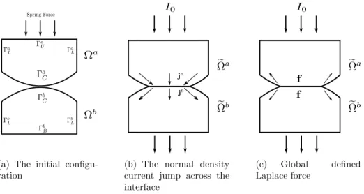
When the circuit breaker is close (the electrodes are in contact with a common area _A), the current ﬂows across the interface governing by two main principles: conservation of the normal density current and a null potential jump across the interface, as represented at Figure 2 (a). Moreover, the electric current generate a Laplace force ( as represented at Figure 2 (b) ), repulsive at contact zone, which plays the fundamental role of a circuit breaker mechanism. When current increases, the Laplace force increases and the geomet-rical design of the apparatus results to a reduction of the contact surface till we reach a complete separation. The present chapter is dedicated to the construction of the electrical model where one computes the electric and the magnetic ﬁeld in function of the contact surface.

(a) The initial conﬁ gu-ration

(b) The normal density current jump across the interface

(c) Global deﬁned Laplace force

Figure 2: Electric-Magnetic problem outline

2.2 Mathematical modelling

A medium voltage circuit breaker is designed to work with continuous or low frequency current (for instance 50 Hz). It results that a common approach use the low frequency approximation (see Rappaz and Touzani [2]) where we neglect the displacement current and the induction eﬀect. Consequently, we use the standard scalar potential formulation and denote byφthe scalar electrical potential whileE=−∇φstands for the electricﬁeld andj=σE represents the current density withσ >0 the conductivity we suppose to be constant for the sake of simplicity. When necessary, we shall use the notations φℓ_, _Eℓ_,

jℓ_, _ℓ₌_{a, b} _{to characterise the quantities associated to domain} _Ω_�ℓ _{respectively. Moreover} component of the global vector writes j = �ja_,_jb� ₌ �₍_ja

1, j2a,), � jb 1, j2b, �� , E = �Ea_,_Eb�

(4)

andφ=�φa_,_φb�_.

Assuming that no electrical charge are present in the domain, the density current conser-vation writes

∇·j= 0, inΩ� (1)

and deduce the scalar electrical potential formulation

−∇·(σ_∇φ) = 0, in Ω� (2)

We equipped the equation with the following boundary conditions: φ= 0 on the basement �

ΓB, a uniform distribution on the upper side

j_·n= I0

|�ΓU|

(3)

with I0 the intensity current while we prescribe an homogeneous Neumann condition for the rest of the boundary to model that fact that no current crosses the boundary which are in contact with the vacuum.

2.3 The two domains formulation

From a practical point of view, the electrical problem will be seen as the coupling of two subproblems deﬁned in each subdomain. Here classical Sobolev spaces are used to obtain a variational formulation. We rewrite equation (2) in the following way: ﬁndφa _and _φb

such that

−∇·(σ_∇φℓ) = 0, in Ω�ℓ (4)

withφb_{= 0 on the basement}_Γ�

B, ja·na =

I0

|Γ�U|

while we assume homogeneous Neumann condition condition for the vacuum boundary. To complete the new model, we prescribe continuity for the normal current and potential across the contact zone:

ja·na+jb·nb= 0, φa=φb, on A. (5) Indeed, assume thatφ∈H1₍_Ω�₎_∩_C0₍_Ω�_{) is a solution of the one domain problem then from} the continuity we deduce φa ₌ _φb _on _A_{. On the other hand, let} _ψ _∈ _H1

0(Ω�), integration by part yields 0 = � � Ω σ_∇φ_∇ψdx= � � Ωa σ_∇φ_∇ψdx+ � � Ωb σ_∇φ_∇ψdx

Now, integration by parts on each subdomains provide

0 = � � Ωa−∇· (σ∇φ)ψdx+ � � Ωb−∇· (σ∇φ)ψdx+ � A σ(ja·na+jb·nb)ψds.

(5)

Relation (4) yields that for anyψ ∈H1 0(Ω�) we have � A σ(ja·na+jb·nb)ψds= 0 which implies ja_·_na₊_jb_·_nb _{= 0} .

3 THE MAGNETICAL FIELD

With Ein hand, we deduce the current density jand we aim to compute the associated electrical field to at last deduce the Laplace force. To this end, let us byBthe magnetic inductionfield. For three-dimensional configuration, the Ampère-Maxwell law writes

∇×B= µ0j, in R3 ₍₆₎ withµ0 the magnetic permeability in the vacuum or non-ferromagnetic material.

Assuming invariance following thezdirection and that the magnetic ﬁeld only depend on

xandy, we deduce that the only non-vanishing component isB(x1.x2) =Bz(x1, x2) and the Amp`ere-Maxwell equation writes

∂2B =µ0j1, −∂1B =µ0j2, inR2 wherejis a given function on R2 _{with compact support.}

Dealing with the rotational operator _∇_× in R2_{, we deduce that} _B _{is also the solution} of problem µ0∇×j = ∇×∇×B = −ΔB (see [2]) with the asymptotic behaviour

B(x) =_O(_|x_|−1_{) when} _|_x_|_{→ ∞}_.

Another alternative is to introduce the potential magnetic vectorAsuch thatB=∇×A whereA is the solution of problem

∇×(∇×A) =−ΔA=µ0j, in R2 with the asymptotic behaviour|A(x)|=O�ln(|x|)�.

However this relationship is not useful for magnetic field computation since the function is defined in the whole domain R2 _{while we just need to determine} _B _{on domain} _Ω�_{. An} alternative approach consists to use the integral representation, namely the Biot-Savart formula. For two-dimensional geometriesΩ�_⊂R2_{(see [3]). The vector potential magnetic} field and the magneticfield at a point xare given by

A(x) = ₋µ0 2π � � Ω j(y) ln(_|x₋y_|)dy (7) B(x) = ∇x×A=− µ0 2π � � Ω j(y)×∇xln(|x−y|)dy, (8)

(6)

for a current j ﬂowing in the direction of e1 and e2 where × represents the external product between two vectors. After some algebraic manipulation, equation (8) writes

B(x) = µ0 2π � � Ω det[j(y),(x₋y)] |x−y|2 dy. (9)

At least, the Laplace force is given by

f =j_×B,

and in our speciﬁc case withB=Be3, the force writes � f1 f2 � =B � j2 −j1 � . (10) 4 MATRICIAL REPRESENTATION 4.1 Representation for Aa eh

Usingﬁnite element methods we will introduce the matricial representation for this prob-lem. We identify the new meshes ofΩ�ℓ _by _T_�ℓ

h, ℓ= a, b, respectively, and To enforce the

Dirichlet condition we use a penalisation method which seems more adapted. Indeed, the contact zone may change with respect to the elasticity problem hence to avoid a new codiﬁcation of the boundary and to reshape the matrix, we always use the same stiﬀ matrix and introduce the Dirichlet condition by multiplying the entries corresponding to the nodes of_Aa

η,h.

I

Figure 3: Discrete active zone deﬁnition The rigid matrix writes

[Aa e] = � Aa eh � φa i,φaj �� i,j=1,...,na while the associated write-hand side is given by

[Θa_] i=    0 _⇐ i_∈_{1, . . . ,n˜a_} � � Γ_Uh I0 |Γ�_Uh|ϕ a i ds, ⇐ i∈{n˜a+ 1, . . . , na}

(7)

Let denote by Ea

η,h the nodes which correspond to domain Aaηh. Once we compute the system matrices at each step, the Dirichlet condition correspondent to_Aa

ηhcan be imposed by substitution method.

Resolution of the elliptic problem turns to solve the simple matricial problem [Aa

e] [Φa] = [Θa]

where [Φa_{] are the unknowns on the nodes.}

4.2 Representation for Ab eh

Since the Dirichlet condition does not change with the iteration, we do not use a penal-ization method for operatorAb

eh and recall thatPi,i= 1,· · ·,n˜

b_{, correspond to the nodes}

ofΩ�b _{except the node of boundary}_Γ�

B. The rigid matrix then writes

� Ab e � = �Ab eh � φb i,φbj �� i,j=1,...,n˜b Let ρb

h be a given constant piecewise function on �ΓaCh characterized by vector [ρ] =

�

ρ1· · ·ω_sb C

�T

. We introduce the Neumann conditions with vector � Θb([ρ])�_i = � T⊂Γ�b Ch � T ρb_hφb_i ds,⇐i∈�1, . . . , nb_C�.

The elliptic problem consist in solving the matricial problem �

Ab e� ��Φb

�

=�Θb�

where �Φ�b� _{are the unknowns on the nodes. We complete the vector setting} �_Φb� ₌

��

Φb�_,₀�_{taking into account the homogeneous boundary condition.}

4.3 Current density and normal projection Setting jℓ

h = ∇φℓh∈Xhℓ, we obtain a constant piecewise vector over Ω�ℓh which represents

the current density ﬁeld. We shall represent the vector in two vectors depending on the coordinates, � jℓ 1 � = � jℓ1,1· · ·jℓnℓ K,1 �T and �jℓ 2 � = � ja1,2· · ·janℓ K,2 �T . that we gather in the matrix form

� jℓ� = � �jℓ 1 � � jℓ 2 � �T .

(8)

We report here the deﬁnition of the matricial expression of the projection following the normal direction. We denote by�Nℓ�_∈Rnℓ

C×2nℓC the matrix of the outwards normals over

Γℓ C and set � Nℓ� =    nℓ h1,1 · · · 0 nℓh1,2 · · · 0 . .. . .. 0 · · · nℓ h nℓ C,1 0 · · · n ℓ h nℓ C,2    We introduce the global matricial representation of�Nℓ�onΩℓ

h:

�

Nℓ� ₌ � �_Nℓ� ₀₀₀ �

with [Na_]_∈_Rnℓ

C×(˜na+na) and�Nb�∈RnℓC×2˜nb.

4.4 Representation for the mappings on contact zone We recall the matricial representation �Cℓ,I�_∈_RnI_×_nℓ

C and�CI,ℓ�=�Cℓ,I�T ∈RnℓC×nI for operatorsC_h,ℓ,I_η andC_ηI,_,hℓ respectively

�

Cℓ,I�_ki = �

I

µk(ξ)φℓi(ξ)dξ, k= 1,· · ·, nI, i= 1,· · ·, nℓC.

In the same way, we represent operatorsD_h,ℓ,I_η andDI,_η_,hℓ with�Dℓ,I�_∈_RsI_×_sℓ

C and�DI,ℓ�= � Dℓ,I�T _∈_Rsℓ C×sI with � Dℓ,I�_ki= � I λk(ξ)ϑℓi(ξ)dξ, k = 1,· · · , sI, i= 1,· · · , sℓC.

4.5 The iterative problem within the matricial form

We now give the iterative procedure at the matricial level. Notice that the procedure corresponds to the one one really implemented on computer thus the importance to deﬁne completely all the step. The iterator index isrand we shall compute a sequence of vectors [ν]r _{which shall converge.}

Assume that vector [ν]r _{is known such that [}_ν_]r

k = 0 for the nodes Nk outside of Jη. the procedure is given by the following substeps (we omit subscript k for the sake of simplicity):

1. Compute vector [wa_{] =}�_DI,ℓ�_[_ν_]r

2. Compute [Φa_{] solving problem}

[Aa_e] [Φa] = [Θa] with penalization with respect to [ωa_].

(9)

3. Compute [ja_{] with}_∇_φa h and compute [ρa] = [Na][ja]. 4. Compute [τ] =�Dℓ,I�_[_ρa_{] and [}_ρb_{] =}₋�_Dℓ,I�_[_τ_] 5. Compute�Φb�₌��_Φ�b�_,₀�_solving � Ab_e� ��Φb�=�Θb�

6. Extract [ωb_{] from}�_Φb�_{and compute [˜}_ν_{] =}�_Cℓ,I�_[_ωb_{] where we cancel the entries} _k

which correspond to the nodesNk outside ofJη. 7. Compute the new vector [ν]r+1₌_θ_[_ν_]r_{+ (1}₋_θ_)[˜_ν_]

We repeat the algorithm till we satisfy the convergence criterion. 5 NUMERICAL SIMULATION

5.1 One domain case

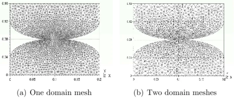
We begin by considering the case with one domain. Once the length of Jη is determined we solve the discrete electric problem on the domain have the conﬁguration of the two electrodes in contact, Figure 4. We this domain we do not have to worry about the potential continuity at the contact zone. More, these results will give us a benchmark for the later results obtained with the domain decomposition technique and two domains. For this case we considerm(Jη) = 0.0468 and I0= 10kA.

(a) One domain mesh (b) Two domain meshes Figure 4: Domain mesh

Figure 4 shows that with both strategies we obtain very similar results. This validates the results and in particular our technique for passing information between the domains at domain decomposition method.

At Figures 6 and 7 although the range of values are similar, the observed difference is justified by the mesh difference, since the density is approximated numerically in the

(10)

(a) One domain (b) Two domains Figure 5: Potential scalarﬁeld

(a) One domain (b) Two domains Figure 6: Current densityﬁeld

barycentric coordinates in the element from the given potential at the nodes. Also in theseﬁgures we can see the continuity of density at the the contact zone.

The magnetic induction (component following e3 ) is exactly the same Figure 8. About Laplace force there is a reduction though the magnitude is equal and we have almost the symmetry between the two domains Figure 9, where we recall again that the meshes are not symmetrical and that the Laplace force are calculated is approximated numerically in the barycentric coordinates in the element.

At this section we will analyse the numerical solutions produced at electro-magnetic state when the electrodes are in contact through a determined active zone.

For each numerical problem we determine the volume repulsive force generated for a given

m(J) and intensity currentI0, for two proﬁles cases: elliptic and circular. 5.2 Two domains case

We are interested to analysing the proﬁles of the potential contact zone: elliptic and circular. From [4] we use two intensity values I = 10 kA , I = 20 kA, I = 40 kA and

(11)

Figure 7: Zoom of current densityﬁeld at contact zone

(a) One domain (b) Two domains Figure 8: Magnetic induction (component followinge3 )

(a) One domain (b) Two domains Figure 9: Laplace force

I = 60 kA. We consider that a inicial spring force has applied, characterized by

F =κ_×α(N) (11)

with

κ= E×A

L (12)

named the axial stiﬀness, where

(12)

A, the contact zone area (in m2_{) and}

Lthe circuit breaker height (in m).

The value αrepresents the vertical displacement, so here we will suppose α_≤0.2 5.3 Elliptic proﬁle

Here we consider a contact with a elliptic proﬁle with a contact zone lengthm(Jη) = 0.032, corresponding to α= 0.1 .

Table 1: Repulsive force generated with an elliptic proﬁle and large active zone and test for several values ofθ

intensity current (A) θ repulsive force generated (N)

1×104 _.₁₂₅ ₄₄_.₅₃ 1_×104 _.₂₅ ₄₄_.₅₃ 1_×104 _.₅ ₄₄_.₅₃ 2×104 _.₁₂₅ ₁₇₈_.₁₃ 2_×104 _.₂₅ ₁₇₈_.₁₃ 2_×104 _.₅ ₁₇₈_.₁₃ 4×104 _.₁₂₅ ₇₁₂_.₅₃ 4_×104 _.₂₅ ₇₁₂_.₅₃ 4_×104 _.₅ ₇₁₂_.₅₃ 6×104 _.₁₂₅ ₁₆₀₃_.₂ 6_×104 _.₂₅ ₁₆₀₃_.₂ 6_×104 _.₅ ₁₆₀₃_.₂

From the results explained at Table 1, we can expect a function of the kind

(13)

Using least squares method we obtain a1= 44.53. represented at Figure 10. 0 500 1000 1500 2000 2500 3000 0 1 2 3 4 5 6 Force (N) Itensity ×104 _(A) Fit line Repulsive force generated

× ×

×

Figure 10: Elliptic proﬁle and large active zone: Repulsive force generated ”×” and least squares approx-imation ”line”

Now we test a reduction of the contact zone,m(Jη) = 0.012, corresponding to α= 0.01.

Table 2: Repulsive force generated with an elliptic proﬁle and small active zone intensity current (A) repulsive force generated (N)

1_×104 ₅₁_.₁

2×104 ₂₀₄_.₄₂

4×104 ₈₁₇_.₆₉

6_×104 ₁₈₃₉_.₈₂

(14)

Using least squares method we obtain a2= 51.1. represented at Figure 11. 0 500 1000 1500 2000 2500 3000 0 1 2 3 4 5 6 Force (N) Itensity ×104 _(A) Fit line Repulsive force generated

× ×

×

Figure 11: Elliptic proﬁle and small active zone: Repulsive force generated ”×” and least squares ap-proximation ”line”

6 Circular proﬁle

Here we begin by consider a circular contact proﬁle after deformation withm(Jη) = 0.045, corresponding to α= 0.1.

fR(I0) =a3I02. (15)

Using least squares method we obtain

a3= 186.71. represented at Figure 12.

Like as above Consider now a small contact zone, m(Jη) = 0.016, corresponding to

α= 0.01.

(15)

Table 3: Repulsive force generated with an circular proﬁle and large active zone intensity current (A) repulsive force generated (N)

1_×104 ₁₈₆_.₇₁ 2×104 ₇₄₆_.₈₅ 4_×104 ₂₉₈₇_.₄₂ 6_×104 ₆₇₂₁_.₆₉ 0 2000 4000 6000 8000 10000 0 1 2 3 4 5 6 Force (N) Itensity _×104 _(A) Fit line Repulsive force generated

× ×

×

Figure 12: Circular proﬁle and large active zone: Repulsive force generated ”×” and least squares approximation ”line”

Using least squares method we obtain

a4= 200.35. represented at Figure 13.

Observingfigures we note that the repulsive force depends on the electrode profile being more important in the case of a circular profile. It also appears that the repulsive force increases as the extent of the active area decreases.

(16)

Table 4: Repulsive force generated with an circular proﬁle and small active zone intensity current (A) repulsive force generated (N)

1_×104 ₂₀₀_.₃₄ 2×104 ₈₀₁_.₃₉ 4_×104 ₃₂₀₅_.₅₉ 6_×104 ₇₂₁₂_.₅₉ 0 2000 4000 6000 8000 10000 0 1 2 3 4 5 6 Force (N) Itensity _×104 _(A) Fit line Repulsive force generated

× ×

×

Figure 13: Circular proﬁle and small active zone: Repulsive force generated ”×” and least squares approximation ”line”

7 CONCLUSION

From the results we have obtained can conclude that the proposed domain decomposi-tion algorithm converges to a continuous soludecomposi-tion of the scalar electrical potential ﬁeld, independently of parameterθ.

Comparing figures 10 - 12 and 11 - 13 we note that the repulsive force depends on the electrode profile and being more important in the case of a circular profile.

With this tests, we can also observe that the repulsive force is inversely proportional to the length of the active zone.

(17)

real problem is three-dimensional and brings more diﬃculties. The contact zone is more complex and the computational eﬀort is larger.

8 REFERENCES

[1] R. Garzon.High Voltage Circuit Breakers: Design and Applications. Pitman Advanced Publishing Program, Boston, 1985.

[2] J. Rappaz R. Touzani. Mathematical Models for Eddy Currents and Magnetostatics With Selected Applications. Springer - Scientiﬁc Computation, New-York, 2014. [3] J.-C. Suh. The evaluation of the biot-savart integral. Journal of Engineering

Mathe-matics, pages 375–395, 2000.

[4] A. Slama. Modlisation des sources de courant en mouvement et des eﬀorts lectro-dynamiques dans les appareils de coupure. PhD gnie electrique, Institut National Polytechnique de Grenoble - France, 2001.