Systems: Integrating Conceptual
Clustering with a Relational
Database Management System
Konstantina Lepinioti
Bournemouth UniversityA thesis submitted in partial fulfillment of the requirements of
Bournemouth University for the degree of Doctor of Philosophy
consults it is understood to recognise that its copyright rests with its author and due acknowledgment must always be made of the use of any material contained in, or derived from, this thesis.
I would like to express my appreciation to all the people who have contributed, directly or indirectly, to the completion of this thesis. Above all, I would like to thank my supervisor, Doctor Stephen McK-earney, for being a great support and inspiration all these years. I am grateful to him for engaging my interest in the area of data mining and databases. I am also grateful to him for guiding and encouraging me from the beginning until the end of this journey.
I would like to thank my second supervisor, Professor Sally McKlean, for her contribution in this work, mainly, in the early years of my research.
I would also like to thank my parents (Stergios and Eleni) and my sisters (Zoe and Ioanna) for their support and understanding, partic-ularly, at the difficult times of anger and frustration.
I would like to express my thanks to the data mining group of the British Telecom Ipswich research centre, which funded my MPhil re-search that lead to this thesis.
Finally, I would like to thank Sudipto Guha, Vipin Kumar and Michael Steinbach for providing the source code for the ROCK algorithm and Periklis Andritsos for providing executables for the LIMBO algorithm.
Many clustering algorithms have been developed and improved over the years to cater for large scale data clustering. However, much of this work has been in developing numeric based algorithms that use efficient summarisations to scale to large data sets. There is a grow-ing need for scalable categorical clustergrow-ing algorithms as, although numeric based algorithms can be adapted to categorical data, they do not always produce good results. This thesis presents a categorical conceptual clustering algorithm that can scale to large data sets using appropriate data summarisations.
Data mining is distinguished from machine learning by the use of larger data sets that are often stored in database management systems (DBMSs). Many clustering algorithms require data to be extracted from the DBMS and reformatted for input to the algorithm. This thesis presents an approach that integrates conceptual clustering with a DBMS. The presented approach makes the algorithm main memory independent and supports on-line data mining.
Nomenclature xi
1 Introduction 1
1.1 Contributions . . . 3
1.2 Organisation of the Thesis . . . 4
2 Clustering 6 2.1 Definition . . . 7
2.2 Data Types . . . 7
2.3 Similarity and Dissimilarity . . . 9
2.4 Clustering Techniques . . . 10
2.4.1 Partitional and Hierarchical Clustering . . . 10
2.4.1.1 Agglomerative Clustering . . . 13
2.4.1.2 Divisive Clustering . . . 13
2.4.2 Distance Based Clustering . . . 14
2.4.3 Categorical Data Clustering . . . 17
2.4.4 Other Clustering Techniques . . . 21
2.6 Large Scale Clustering of Categorical Data . . . 30 2.6.1 K-modes . . . 31 2.6.2 ROCK . . . 33 2.6.3 LIMBO . . . 37 2.6.4 Summary . . . 43 2.7 Conceptual Clustering . . . 44 2.7.1 Cobweb . . . 45 2.7.2 Discussion . . . 49 3 CLIMIS Clustering 53 3.1 Category Utility . . . 54
3.2 The CLIMIS Clustering Algorithm . . . 56
3.2.1 Cluster Summarisation . . . 57 3.2.2 CLIMIS Tree . . . 59 3.2.3 CLIMIS Algorithm . . . 62 3.3 Contributions . . . 66 4 Evaluation of CLIMIS 68 4.1 Algorithms . . . 68 4.2 Data Sets . . . 71 4.3 Quality . . . 77 4.4 Scalability . . . 82
4.4.1 CLIMIS versus Cobweb . . . 84
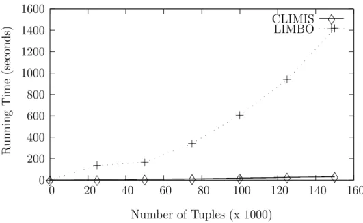
4.4.2 CLIMIS versus LIMBO . . . 86
4.4.3 CLIMIS versus ROCK . . . 91
5 Implementation 98
5.1 Logical Architecture Packages . . . 98
5.1.1 Data Clustering . . . 99 5.1.2 Prediction . . . 99 5.1.3 Data management . . . 103 5.2 Input/Output . . . 103 5.2.1 Input . . . 103 5.2.2 Output . . . 105
6 Integrating Data Mining with the DBMS 107 6.1 Reasons for Integrating Data Mining with a DBMS . . . 108
6.1.1 Simplifying the KDD Process . . . 108
6.1.2 Achieving Main Memory Independence . . . 110
6.1.3 Supporting On-line Data Mining . . . 111
6.2 Considerations when Integrating an Algorithm with a DBMS . . . 112
6.2.1 The Data . . . 112
6.2.2 The Resources . . . 115
6.3 Approaches to Integrating Data Mining with a DBMS . . . 116
6.3.1 Treating the DBMS as a Repository . . . 118
6.3.2 Changing the DBMS . . . 119
6.3.3 Mapping Data Mining to SQL and Database Relations . . 120
6.4 Discussion . . . 124
7 Integrating CLIMIS with a DBMS 126 7.1 The Cobweb/IDX Approach . . . 126
7.2.1 CLIMIS Tree . . . 132
7.2.2 Mapping the CLIMIS Tree to the Relational Data Model . 135 7.2.3 Cache Replacement Policies . . . 137
7.2.4 PD-structure . . . 138
7.2.5 Interaction with the CLIMIS Algorithm . . . 141
7.2.6 Size of the Cache Data Structures . . . 144
7.2.7 Full DBMS Interface . . . 146
8 Evaluation of the CLIMIS Data Structures 147 8.1 CLIMIS Tree . . . 148 8.2 PD-structure . . . 155 8.3 Conclusion . . . 159 9 Conclusions 161 9.1 Contributions . . . 162 9.2 Limitations . . . 163 9.3 Future Work . . . 163
9.3.1 Using CLIMIS to Scale ITERATE . . . 164
9.3.2 Extending CLIMIS to Relational Data Mining . . . 164
9.3.3 Extending CLIMIS to Numeric and Mixed Data . . . 164
A Experiments with ROCK and the Congressional Votes Data Set166
B Experiments with ROCK and the Mushroom Data Set 168
C Experiments with LIMBO and Different φ Values 170
2.1 Mapping Categorical Data to Boolean . . . 18
2.2 A CF-tree Example (Zhang,1997) . . . 26
2.3 The Cobweb Tree . . . 47
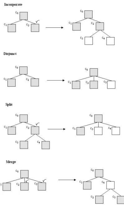
2.4 Cobweb Operators . . . 50
3.1 CLIMIS Tree . . . 60
3.2 PD-Structure . . . 61
3.3 Application of the Cutoff Operator . . . 65
4.1 CLIMIS versus Weka (Cobweb): Increasing the number of tuples . 85 4.2 CLIMIS versus Weka (Cobweb): Increasing the number of attributes 86 4.3 CLIMIS versus Weka (Cobweb): Using the cutoff parameter . . . 87
4.4 CLIMIS versus LIMBO: Increasing the number of tuples . . . 88
4.5 CLIMIS versus LIMBO Phase 1: Increasing the number of tuples 89 4.6 CLIMIS versus LIMBO: Increasing the number of attributes . . . 90
4.7 CLIMIS: Increasing clusters in the data set . . . 91
4.8 CLIMIS versus ROCK: Increasing the number of tuples . . . 92
4.9 CLIMIS versus ROCK: Increasing the number of attributes . . . 93
4.11 CLIMIS: Increasing the number of tuples . . . 95
5.1 Data Clustering - Class Diagram . . . 100
5.2 Tree - Class Diagram . . . 101
5.3 PD-structure - Class Diagram . . . 102
5.4 Data Management - Class Diagram . . . 104
5.5 Relations Used by CLIMIS . . . 106
6.1 Cross-Industry Standard Process for Data Mining (Shearer,2000) 109 6.2 Sarawagi’s Alternatives to Integrating a Data Mining Algorithm with a DBMS . . . 117
6.3 Example of Decision Tree . . . 120
6.4 MIND: Data Summarisation . . . 122
6.5 MIND: Best Split . . . 122
7.1 Cobweb/IDX Update Process . . . 129
7.2 Cobweb/IDX Search Process . . . 130
7.3 Conceptual Clustering Tree . . . 133
7.4 CLIMIS Tree as a Cache . . . 134
7.5 PD-structure . . . 139 7.6 Get Children . . . 141 7.7 Implement Incorporate . . . 142 7.8 Implement Disjunct . . . 142 7.9 Implement Split . . . 143 7.10 Implement Merge . . . 143
7.11 Getting Attribute Value Probabilities for Merge from the
PD-structure . . . 143
7.12 Size of the CLIMIS Tree . . . 145
7.13 Size of the PD-structure . . . 145
8.1 Hit Rate with Regard to Reducing Size of Cache . . . 149
8.2 Hit Rate with Regard to Increasing No. of Tuples . . . 151
8.3 Hit Rate with Regard to Increasing No. of Attributes . . . 152
8.4 Skewed versus Balanced Tree . . . 154
8.5 Hit Rate with Regard to Reducing Size of PD-structure . . . 156
8.6 Hit Rate with Regard to Increasing No. of Attributes . . . 157
Introduction
Clustering is a widely used data mining technique that has applications in areas such as marketing, to identify similar customer behaviour, and the WWW, to discover similar access patterns (Berry & Linoff, 2004;Dunham, 2003). The goal of clustering is to discover natural clusters in unclassified data that can then be studied to learn interesting rules (Everitt, 1993).
Many clustering algorithms have been developed and improved over the years for the purpose of analysing large data sets. Some of the most successful large scale clustering algorithms are numeric based algorithms that use efficient summarisations of the data. However, large data sets often contain categorical data that is not as easy to summarise.
Categorical clustering algorithms have proved more difficult to scale to large data sets (Andritsos et al., 2004; Zhang et al., 2000). One approach to achieve scalability when clustering categorical data is to use numeric based algorithms. This solution is not always successful in discovering a good clustering as it may fail to discover the natural clusters in the data (Guha et al., 2000).
is the conceptual clustering algorithm Cobweb (Fisher, 1987). As a conceptual clustering algorithm, Cobweb organises data into categories that maximise the similarity of data in the same category and minimise the similarity of data in different categories (Michalski,1980). Cobweb has been successfully used in pre-dicting missing data (Biswas et al.,1998) and personalisation of internet services
(Paliouras et al., 1999). Furthermore, some of its features that work well with
large data sets have been used in more recent algorithms, for example Cobweb’s ability to process data sequentially (Zhang, 1997).
The main disadvantage of Cobweb as a conceptual clustering algorithm is its inability to scale to large data sets. The aim of this thesis is to investigate if it is possible to scale conceptual clustering to large data sets of categorical data. Most of the data used in clustering exists in databases. Unfortunately, like other data mining techniques, clustering is performed, mainly, outside the DBMS using algorithms that are restricted by the available resources (Dunkel
et al., 1997; Netz et al., 2000; Ordonez & Omiecinski, 2004). As a result, the
overall data mining task can be complex. The user has to extract the data from its storage environment and be aware of any resource limitations (Kepner & Kim, 2003) to be able to apply the clustering algorithm and obtain a clustering. Another aim of this thesis is to investigate if it is possible to make conceptual clustering main memory independent and applicable directly to data that exists in a DBMS.
Data stored in a database is normally updated frequently creating a need for dynamic or on-line data mining. Unfortunately, many of the data mining
al-gorithms perform static data mining (Dunham, 2003). For clustering this means that once an algorithm builds a set of clusters these cannot be updated. In ad-dition, data stored in a database is of a variety of types. Therefore, clustering algorithms that can handle different data types are more suitable. There are clustering algorithms that can handle data of different data types (mixed data) but the majority are one type algorithms, often numeric based. Also, data stored in a database is structured data following a conceptual and logical model (Date,
1995;Elmasri & Navathe,2000). There are already examples of work in the
liter-ature that attempted to use either one or the other model to support data mining
(Ketterlin et al.,1995), but most of the clustering algorithms in the literature are
applicable to data that exists in a flat file form. Another aim of this thesis is to identify clustering algorithm properties that suit the characteristics of data that exists in a DBMS.
Algorithms used in a DBMS, for example indexing algorithms (Sellis et al.,
1987), require minimum input from a database user. Another aim of this thesis is to identify clustering algorithm properties that suit a DBMS.
1.1
Contributions
This thesis makes the following contributions:
• Proposes CLIMIS, a scalable conceptual clustering algorithm for categorical data.
• Shows how conceptual clustering for categorical data can be scaled to large data sets by using data summarisations appropriate for categorical data.
• Shows how conceptual clustering for categorical data can be scaled to large data sets without incurring any loss in the quality of the clustering results. • Shows how to achieve main memory independence by using a cache that
integrates conceptual clustering with a relational DBMS.
• Uses an approach to clustering that supports on-line clustering.
• Uses an approach to clustering that can be extended to mixed data and has immediate database applications.
• Uses an approach to clustering that can be applied to structured data. • Uses an approach to clustering that is possible to apply directly to data
that exists in a DBMS.
1.2
Organisation of the Thesis
The organisation of this thesis is as follows. Chapter 2 presents a discussion of representative clustering techniques and algorithms. Chapter 3 is a discussion of our algorithm CLIMIS and how it scales to large data sets. Chapter 4 presents an evaluation of CLIMIS and compares it with other algorithms that also have been developed for clustering large categorical data sets. Chapter 5 presents designs that reflect the implementation of CLIMIS. Chapter 6 is a discussion of different motivations, approaches and considerations when integrating an algorithm with a DBMS. Chapter 7 discusses how we integrated CLIMIS with a relational DBMS. Chapter 8 presents an evaluation of the extended CLIMIS and the thesis ends
with chapter 9, which includes the conclusions on this work and the ways we plan to extent our work with future research.
Clustering
Clustering is a research area in the fields of machine learning, statistics, databases and data mining. Clustering is employed in a number fields to infer knowledge from data. For example, clustering is used in marketing for identifying customer segments, in biology for grouping plants and animals based on their features, in telecommunications and insurance for fraud detection and in relation to the world wide web to discover groups of similar access patterns based on web log data. The problem of clustering data sets is that, quite often, the available clustering algorithms do not satisfy the clustering requirements of these fields. One of the clustering requirements is to cluster large data sets as the data collected in these fields increases every year. Dunham(2003) suggests that data doubles every year, but useful information seems to be decreasing.
This chapter starts by discussing various approaches to clustering and their problems with clustering large data sets. The chapter then presents how these approaches have been adapted to cluster large data sets.
2.1
Definition
Clustering is the grouping of a set of data into subsets, called clusters, such that the data are similar when they appear in the same cluster and dissimilar when they appear in different clusters (Everitt, 1993; Fasulo, 1999; Fraley & Raftery,
1998; Hartigan, 1975; Hinneburg & Keim, 1999). A good clustering of a given
data set is one that maximises the similarity between data in the same cluster and dissimilarity between data in different clusters. A clustering algorithm normally seeks for a good trade off between the two.
2.2
Data Types
As already mentioned, earlier in this thesis, most of the data used in data mining comes from a database. Interestingly, the data mining view of data, and therefore clustering, is different to that of databases.
A database stores data as a set of relations. A relation is a set of tuples and each tuple is a set of attribute values. Each attribute value has a data type determined by the data type of the attribute.
Two major data types that are found in databases, particularly commer-cial databases, are numeric and categorical data. The data mining view of data is based on statistics and is more complex than the database view of data. A statistical view of numeric and categorical data, identifies numeric and categor-ical (also known as categoric) as two main categories of data that also include subcategories. Two subcategories of numeric are ratio and interval data and two subcategories of categorical are nominal and ordinal data (Hastie et al., 2001;
Pyle,1999;Stevens,1946). Each subcategory indicates important characteristics of the data.
• Numeric Data
– Ratio Data: Ratio data is numbers and is not categorised. Ratio
data is on a scale that has a meaningful zero and a common distance between individual points. Data that can be counted such as money and age is normally ratio data. For example, £50 is twice as much compared to£25.
– Interval Data: Unlike ratio data, interval data is on a scale with no
common distance between individual points. For example, the Cel-sius temperature scale is considered to be an interval scale because 50 degrees Celsius is not twice as hot as 25 degrees Celsius.
• Categoric Data
– Nominal Data: Data is considered to be nominal when it is possible
to put it into categories but these categories cannot be put into any order. Examples of nominal data are: nationality, gender and religion.
– Ordinal Data: Ordinal data can be put into categories. Unlike nominal
data, ordinal data categories can be put into an order. Examples of ordinal data are:
-∗ rates (A, B, C, D),
∗ attitudes (strongly agree, agree, disagree, strongly disagree), and ∗ body mass index categories (anorexic, slim, normal, overweight,
This statistical view of data is important for data mining as each data type may require different analysis and have different limitations when it comes to large data analysis. For example, the analysis of nominal data is considered more complex because it happens at attribute value level, whereas the analysis of numeric data happens at attribute level.
2.3
Similarity and Dissimilarity
A clustering algorithm makes use of a similarity or dissimilarity measure to quan-tify the quality of a clustering. The terms similarity and dissimilarity are often used interchangeably (Han & Kamber, 2000;Milligan, 1996). This is because, in the literature, particularly with numeric data, dissimilarity is viewed as another aspect of similarity (Gowda & Diday, 1992). In general, a similarity measure shows the strength of the relationship between two objects. A higher measure-ment indicates a greater similarity between two objects. A dissimilarity measure shows the distance between two objects. A lower measurement indicates a lesser dissimilarity between two objects.
The suitability of a measure for the analysis of a data set depends on the type of the data. For example, distance based measures are particularly suitable for clustering numeric data as numeric data can be easily viewed as points in a metric space, metric data.
2.4
Clustering Techniques
Clustering algorithms follow different clustering techniques. This section dis-cusses different clustering techniques and examples of algorithms that follow these techniques.
2.4.1
Partitional and Hierarchical Clustering
A clustering algorithm can be described as partitional or hierarchical depending on the approach it follows to produce a set of clusters (Jain & Dubes, 1988).
Partitional Clustering
Given a databaseDofntuples and an input numberkthat represents the number of desired clusters, a partitional algorithm applies a measure and partitions the data into a flat arrangement of k clusters.
A well known partitional algorithm is the k-means algorithm (MacQueen,
1967). The k-means algorithm is a distance based algorithm that views data as points in a metric space (discussed in detail in section 2.4.2). Furthermore, k-means represents a cluster by a centroid. A definition of a centroid is given by
Al-Harbi & Rayward-Smith (2006) as follows:
Definition 1 Given any set of points, C, in a metric space, M, with metric, d,
a point ˆc∈M is called a centroid if
X
x∈C
where d(ˆc, x) represents the distance between two points. Note that the centroid ˆc is not necessarily an element ofC.
There are different variations and extensions of the k-means algorithm
(Huang, 1998; Kanungo et al., 2002; Pelleg & Moore, 2000). The original k
-means algorithm that other algorithms have been based on follows the steps shown below:
1. Randomly select k initial centroids to represent k clusters. 2. Assign all tuples to their closest centroid using
a similarity/dissimilarity measure.
3. Recalculate the centroids of the clusters.
4. Reassign the tuples according to the new centroids. 5. Repeat 3 and 4 until the same tuples are assigned
to the same clusters in consecutive iterations.
Han & Kamber (2000) give the complexity of k-means as O(nkt), where
n is the number of tuples to be clustered, k is the number of clusters desired and t is the number of iterations. To achieve the same clusters in consecutive iterations and produce a set of clusters, the algorithm may require a high number of iterations.
Another partitional algorithm, similar to k-means, is the k-medoids algo-rithm, which is also known as PAM (Partitioning Around Medoids) (Kaufman &
Rousseuw, 1990). The k-medoids algorithm follows similar steps to k-means. It
looks for a good set of clusters through iterations and at every iteration it resets the medoids and reassigns the points to the best clusters. The main difference between the two algorithms is thatk-means uses a mean to represent the centre of
the cluster, whereask-medoids uses a medoid. A medoid is an object that ideally is the most central object in the cluster: A point ˆm ∈ M is called a medoid if it minimises the objective function, P
x∈Cd( ˆm, x) (Mirkin, 2005). The medoid
must itself be an element of C.
An advantage of thek-medoids algorithms is that it is less sensitive to any noise or outliers than thek-means algorithm (Al-Zoubi,2009;Dehuri et al.,2006;
Han & Kamber,2000;Zhang & Couloigner,2005). The reason is that a medoid is
less affected by an outlier or other extreme values than a mean. A disadvantage of the k-medoids algorithm is that it is costly and only applicable to small data sets (Han & Kamber, 2000).
Part of the research on partitional algorithms has focused on scaling par-titional algorithms to large data sets. An example of a parpar-titional algorithm designed to cluster large data sets is CLARA. CLARA is based on k-medoids and uses a sampling based method to deal with large data sets (Kaufman &
Rousseuw, 1990). It draws a random sample from the original data set and then
applies the k-medoids algorithm. To produce a better clustering partition, the algorithm applies the same process a number of times. According to Han &
Kamber (2000), CLARA’s effectiveness depends upon the size of the sample.
CLARANS is a more recent algorithm also based on k-medoids and sam-pling (Ng & Han, 1994, 2002). Unlike CLARA, they use a dynamic approach to sampling. The algorithm starts with an original clustering partition based on a random sample that they call the current clustering. When the algorithm replaces a single medoid with a medoid randomly drawn from the data set, the new clustering partition, called neighbour, is compared to the current partition
of neighboursdepending on an input parameter decided by the user. CLARANS, according toHan & Kamber(2000), shows better quality than CLARA, but worst complexity.
Hierarchical Clustering
Hierarchical clustering is different from the partitional approach in that, tradi-tionally, it requires no input clusters and builds clusters at different levels of a hierarchy. The output of the hierarchical approach is a dendrogram (tree) that includes clusters at different levels of generalisation or specialisation.
A hierarchical algorithm can follow an agglomerative or divisive approach to clustering.
2.4.1.1 Agglomerative Clustering
Agglomerative clustering follows a bottom up approach to clustering (Duda & Hart,1973). It starts with singleton clusters. If the data set containsntuples, the algorithm starts withnclusters. The algorithm gradually merges the most similar pair of clusters to form a larger cluster until all data is covered by a universal single cluster. An example of an agglomerative algorithm is AGNES (Han & Kamber,
2000; Kaufman & Rousseuw, 1990). AGNES starts with singleton clusters and
creates a dendrogram (tree) of clusters by gradually merging clusters whenever the similarity between them is greater than a given threshold.
2.4.1.2 Divisive Clustering
A divisive clustering algorithm starts with one cluster that covers all the cases. The algorithm splits clusters into smaller ones until every cluster is a singleton and
covers only one tuple. An example of an early divisive algorithm is DIANA (Han
& Kamber,2000;Kaufman & Rousseuw,1990). The algorithm starts with a single
cluster that covers all the data and gradually splits it into smaller clusters by applying a measurement function that indicates the furthest nearest-neighbours. There are algorithms that have combined the partitional and hierarchical approach in order to achieve applicability to larger data sets. For example, the original agglomerative approach started with every point being a cluster on its own. The evaluation process that indicated which clusters to merge was an ex-pensive process. As a result, more recent algorithms that follow the agglomerative approach start with k number of clusters, like the partitional approach, instead of n clusters (Andritsos, 2004).
ITERATE (Biswas et al., 1998) is another example of an algorithm that combines the hierarchical and partitional approach. ITERATE starts with a di-visive algorithm that produces a clustering tree. Based on a measure of clustering quality, a set of clusters are picked from a level of the tree and they are used as an input to a partitional phase of the algorithm to improve the clustering quality. The sections that follow discuss hierarchical algorithms or algorithms that combine the partitional and hierarchical approach as they have been more suc-cessful at clustering large data sets.
2.4.2
Distance Based Clustering
A large number of algorithms, includingk-means, are described as distance based clustering because they view data as points in a metric space. The similarity or dissimilarity between two points ˆx and ˆy, both in a metric space M, is
evalu-ated by measuring the distance between them, d(ˆx,yˆ). To measure the distance between points, measures that are known as metricsare used.
Given three data points ˆx,yˆand ˆzall inM, a distance metric should satisfy the following (Han & Kamber, 2000; Kaufman & Rousseuw,1990):
1. d(ˆx,yˆ)≥0
2. d(ˆx,yˆ) = 0 if and only if ˆx= ˆy
3. d(ˆx,yˆ) = d(ˆy,xˆ)
4. d(ˆx,zˆ)≤d(ˆx,yˆ) +d(ˆy,zˆ)
The first condition says that distances are non-negative numbers. The second condition says that the distance of a point to itself is 0. Number 3 in the list is an axiom that reflects the symmetry of the distance function. Number 4 is known as triangle inequality and reflects the fact that the direct distance from a point ˆxto a point ˆz is always equal or shorter to the distance that includes point
ˆ y.
Two well known and widely used distance metrics that satisfy the above re-quirements are theEuclidean distance(equation2.2) and theManhattan distance
(equation 2.3). Euclidean Distance d(ˆx,yˆ) = v u u t m X i=1 (xi−yi)2 (2.2)
Manhattan Distance d(ˆx,yˆ) = m X i=1 |xi−yi| (2.3)
The above equations (equations2.2 and 2.3) can be used for numeric (real valued) data. However, when the data is of the type categorical (nominal) then:
d(ˆx,yˆ) = 0 (ˆx= ˆy) 1 (ˆx6= ˆy) (2.4)
Given a database D with m attributes, A1, A2, . . . , Am, of the type real
valued and categorical (nominal) data, i.e. mixed data, the following extended
Euclidean metric can be used instead (Nguyen & Rayward-Smith, 2008):
d(ˆx,yˆ) =
q
d2
1(ˆx1,yˆ1) +d22(ˆx2,yˆ2) +. . .+d2n(ˆxm,yˆm), (2.5)
where ˆx = (ˆx1,xˆ2, . . . ,xˆm), ˆy = (ˆy1,yˆ2, . . . ,yˆm) and di(ˆxi,yˆi) is |ˆxi −yˆi|
if ˆxi,yˆi ∈ R, otherwise is the 0/1 metric. Generally, with mixed data, it is
important to ensure that no attribute m dominates another with respect to the metric being used. Thus if, for example, one real valued attribute has values in the range 0, . . . ,1,000,000 then the differences in values could be substantial and other attribute values may be insignificant. Thus scaling of data prior to clustering is necessary.
In light of the extended Euclidean metric, an object ˆc is called a centroid if it minimises P
x∈Cd
2.4.3
Categorical Data Clustering
In the literature, often, the term categorical is used to refer to nominal data
(Cristofor & Simovici,2002; Ganti et al.,1999). However, as discussed in section
2.2, there is also ordinal categorical data, which is different to nominal data and requires different analysis. For instance, the 0/1 metric (see equation2.4) may be suitable for nominal and ordinal data but with ordinal data it ignores the ordering. Ordinal data can be encoded into real values (Rayward-Smith, 2007) so that the absolute difference between two encodings represents the distance between the corresponding two ordinal data points (see equation 2.5). This thesis focuses on the nominal categorical data type. In this section, as well as in the sections and chapters that follow this section, the term categorical will refer to the nominal data type only.
Most of the research in clustering has focused on the analysis of numeric data. Less attention has been given to the analysis of categorical data. To make the analysis of categorical data possible, often, the data is transformed to some numeric representation as many of the existing clustering algorithms can deal with numeric data only (Han, 1998).
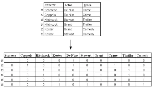
A common transformation approach is to map the categorical data to binary (also referred to as Boolean) data and analyse it as data that can be ordered (metric data) (Pyle, 1999). A binary variable has only two states 0 and 1. The variable 0 indicates that the variable is absent and 1 that it is present (Han &
Kamber, 2000; Li, 2005). For example, in figure 2.1, for attribute Scorsese, 1
indicates that Scorsese is present in t1 and 0 indicates that Scorsese is absent from t2. An example of a mapping of categorical data to binary (Boolean) is
Figure 2.1: Mapping Categorical Data to Boolean
shown in figure 2.1. As the figure shows a Boolean attribute is created for every value in every attribute domain.
Categorical data analysis based on a Boolean mapping is a common ap-proach but has the following disadvantages:
• It adds complexity to the KDD process as it involves more data preparation. • It increases the number of fields.
• It requires knowledge of the entire domain of every attribute before the data mining task starts and, therefore, data mining cannot happen in an ad hoc manner (Chaudhuri et al., 1999).
• It may fail to discover the natural clusters hidden in the data or produce clusters that are not meaningful (Huang,1997; Li & Biswas,2002).
Furthermore,Guha et al.(2000) gives the following example to demonstrate that the use of distance metrics may be inappropriate for categorical data:
Example 1: Consider a market basket database containing the following transactions over items 1, 2, 3, 4, 5 and 6:
1. {1, 2, 3, 5} 2. {2, 3, 4, 5} 3. {1, 4} 4. {6}
A mapping of the transactions to Boolean (0/1) attributes for every item (1, 2, 3, 4, 5 and 6) transforms them and the transactions can be viewed as points:
1. (1, 1, 1, 0, 1, 0) 2. (0, 1, 1, 1, 1, 0) 3. (1, 0, 0, 1, 0, 0) 4. (0, 0, 0, 0, 0, 1)
If the transactions above are viewed as points/clusters in a metric space, following a centroid based agglomerative hierarchical algorithm (Jain & Dubes,
1988), we can apply the Euclidean distance (equation 2.2) and find that points 1 and 2 are the closest points: p(12+ 02+ 02+ 12+ 02+ 02) = √2. Points
1 and 2 are merged into one cluster with centroid (0.5,1,1,0.5,1,0). Points 3 and 4 are also merged as they are closer to each other than to the cluster that includes points 1 and 2. The Euclidean distance between 3 and 4 is√3, whereas their distance from the cluster with the merged points is √4 in both cases. The
problem in this case is that points 3 and 4 correspond to the transactions {1,4} and {6} respectively, which have nothing in common.
As the example above demonstrates, categorical data cannot always be clustered properly by transforming it to Boolean and analysing it as metric data.
Nguyen & Rayward-Smith (2008) recommended using the extended Euclidean
metric (see equation 2.5) for categorical and mixed data. However, even with a
more suitable metric, the approach still suffers the Boolean mapping disadvan-tages listed above.
The research interest on categorical data algorithms has been increasing over the years so categorical data can be clustered without having to be trans-formed (Barbar´a et al., 2002; Chen & Liu, 2005; Cristofor & Simovici, 2002;
Gibson et al., 2000; He et al., 2006). Section 2.6 gives a detailed discussion of
some examples of categorical data algorithms.
Mixed Data Clustering: As categorical data clustering is gradually at-tracting more research interest, mixed data clustering, where categorical and numeric data can be clustered together, becomes more feasible (Li & Biswas,
2002).
There are different approaches to mixed data clustering. One of the ap-proaches involves clustering the categorical and numeric data separately using suitable measurement functions. The resulting clusters are then combined to produce mixed data clusters (He et al., 2005). Another approach to handling mixed data clustering is clustering the categorical and numeric data together but evaluating it separately. To decide on a clustering strategy, the algorithm merges the results of the numeric data evaluation and the categorical data evaluation. An example of an algorithm that follows this approach is thek-prototypes algorithm
(Huang, 1997). To evaluate the similarity between two tuples of mixed data, k-prototypes uses thek-means algorithm for evaluating the numeric data and the k-modes algorithm for evaluating the categorical data (thek-modes algorithm is discussed in section 2.6.1): if sn is the similarity measure of numeric data and
sc is the similarity measure of categorical data then the mixed data similarity is
given by: sn+γsc. Huang (1997) uses γ, a user defined parameter, to balance
the two parts.
A similar approach to that of Huang (1997) is used in Cobweb/3 (
McKu-sick & Thompson, 1990). The Cobweb/3 approach is based on Cobweb and its
extension CLASSIT (Gennari et al., 1989). Cobweb/3 evaluates the similarity between tuples using the category utility (CU) measurement (discussed in chap-ter 3, section 3.1). The algorithm calculates CU for categorical data and CU for numeric data separately and then it combines the two to calculate the similarity between tuples of mixed data: CUmixed =CUcategorical+CUnumeric.
2.4.4
Other Clustering Techniques
Other clustering techniques that will only be discussed briefly in this thesis include the
following:-• Grid-based clustering • Density based clustering • Fuzzy clustering
Grid-based clustering views data as points in space but its difference to distance based clustering is that every dimension of the space is divided into equal intervals to discover subspace clusters (Wang et al., 1997). Grid-based clustering is mainly used with spatial data, which is 2D or 3D data, normally found in geographic information systems.
Density based clustering (Ester et al.,1996) has been developed with spatial data in mind. It uses the concept of density, which is defined as a minimum number of points within a certain distance from each other. It aims to discover clusters with the maximum of density connected points.
In conventional clustering, every tuple belongs to one cluster. Clusters produced in a conventional way, however, may not be well separated. In that case, fuzzy clustering, which allows a tuple to be a member of more that one cluster, is more appropriate (Jain & Dubes,1988;Kaufman & Rousseuw,1990). In fuzzy clustering, a tuple is assigned to a cluster with a degree of cluster membership.
Semi-supervised clustering happens when the data in a data set is not en-tirely or accurately labeled (Bouchachia & Pedrycz, 2006). Supervised learning algorithms (Liu et al., 2002; Martin, 1994) require an output field to guide the analysis process. This output field labels the tuples and any evaluation to clas-sify the tuples is done with regard to the output field. Unsupervised learning algorithms (Iba & Langley, 2001;Oates, 2002;Song et al., 2003;Surdeanu et al.,
2005), on the other hand, do not require an output field to guide their analysis. When the two learning approaches are combined, the learning is referred to as semi-supervised learning (Basu et al., 2006; Kumar et al., 2005).
2.5
Large Scale Clustering
Scalability is one of the main research areas in clustering. There are a number of approaches used to scale clustering algorithms to large data sets:
• Scalability through summarisation • Scalability through compression • Scalability through parallelisation • Scalability through sampling
• Scalability through data partitioning
Scalability Through Summarisation
One approach used to scale existing algorithms to large data sets makes use of data structures that summarise the data set (Serazi et al.,2004). This approach is based on the idea that if sufficient statistics about the clusters are made available, then, the entire clusters are not needed in main memory.
Conventional distance based clustering algorithms, for instance k-means, represent a cluster with the data points that the cluster covers. Unlike those conventional distance based algorithms, there are more recent distance based al-gorithms that summarise the cluster representation and reduce it to the following sufficient statistics: i) a number that shows how many data points the cluster covers, ii) the sum of the data points that the cluster covers, and iii) the sum of the squared data points that the cluster covers. The work presented by Bradley
to be summarised with the term sub-cluster and represent the sub-cluster with statistics that are adequate for computing the metric measure the algorithm uses
(Bradley et al., 1998):
Definition 2 Let {x1, x2, . . . , xN} ⊂ Rn be a set of singleton points to be
com-pressed. The statistics that represent a sub-cluster are the triple(SU M, SU M SQ, N),
where SU M :=PN i=1x i ∈Rn and (SU M SQ) j := PN i=1(x i j)2 for j = 1,2, . . . , d.
A similar cluster representation is used by Zhang (1997). Zhang (1997) introduces the BIRCH algorithm. BIRCH relies on metrics such as the Euclidean
distance to evaluate the clusters and decide on a clustering strategy. BIRCH
represents each cluster as a clustering feature (CF) and provides in this way adequate statistics for the calculation of the metric measure (note that Zhang
(1997) views each data point as a d-dimensional vector):
Definition 3 Given N d-dimensional data points in a cluster {X~i}, where i =
1,2,3, . . . , N, the Clustering Feature (CF) entry of the cluster is defined as a
triple: CF = (N, ~LS, SS), where N is the number of data points in the cluster,
~
LS is the linear sum of the N data points, i.e. PN
i=1X~i and SS is the square
sum of the N data points, i.e. PN
i=1X~i
2
.
Both cluster summarisations, the clustering feature and the cluster sum-marisation of Bradley et al. (1998), use a number, N, to represents the number of points in a cluster. Also, both cluster summarisations have a similar way to represent the sum of the data points in a cluster, LS~ of the clustering feature is equivalent to theSU M of the cluster summarisation ofBradley et al.(1998). The two cluster summarisations differ with regard to SSand SU M SQ. Zhang(1997)
clearly states in her thesis that she views each data point as a d-dimensional vector (Zhang,1997) and that she makes use of the vector dot product operation. With the application of the vector dot product, SS is represented by a number and is more compact than the SU M SQ of Bradley et al.(1998) 1.
Scalability Through Compression
Both of the works that have been discussed above in relation to the summarisa-tion approach (Bradley et al., 1998; Zhang et al., 1996) made use of additional techniques to compress the data further and overcome the problem of limited resources.
Bradley et al.(1998) introduced a system that is based on the idea that in
the data there are regions that are compressible, regions that must be available in main memory and regions that can be discarded. The amount of compression required in their system is determined by the size of the specified memory buffer in the system. In a two phase compression approach, the system first discards from the buffer points that appear unlikely to change cluster membership and then in the second phase they compress the data to produce the cluster summarisations described in the previous section. Unfortunately, Bradley et al. (1998) fail to show any figures that clearly demonstrate the scalability of their algorithm.
The BIRCH algorithm (Zhang et al., 1996) makes use of the clustering
feature (discussed in the previous section) and builds a tree of clusters, the
CF-tree. A CF-tree is a height balanced tree with a user defined parameter called
the branching factor (B for non-leaf nodes and L for leaf nodes) that controls
1SU M SQis represented withdnumbers, wheredis the number of dimensions (attributes)
in the data set, whereas SS is represented with a single number regardless the dimensions in the data set.
the number of entries in a node. A non-leaf node can fit at most B entries and a leaf node can fit at most L entries. For example, in figure2.2 B =L= 3 and a node (non-leaf or leaf) can fit at most 3 entries. Every entry in a leaf node is a
clustering feature (CF). Every entry in a non-leaf node is a summarisation of its
children. Furthermore, a non-leaf node contains pointers to its children and a leaf node contains pointers to the next and previous leaf nodes to support efficient scans.
CF1+CF2+CF3 CF4+CF5
CF1 CF2 CF3 CF4 CF5
T
Figure 2.2: A CF-tree Example (Zhang, 1997)
To incorporate new data into the tree (new CF entry that represents one data point or is the summary of many data points), the algorithm starts from the root and using a metric measure gradually descends to the leaf node that contains the closest CF. The algorithm checks if it can incorporate the new data into the existing CF (sub-cluster). At this point, the algorithm uses a threshold T value. If the diameter of the sub-cluster (the sub-clusters are assumed to be spherical) after incorporation is less than the threshold value, the algorithm proceeds to
update the higher levels of the tree. If the diameter of the sub-cluster after incorporation exceeds the threshold value and there is a free space in the current leaf node, the algorithm stores the new CF entry separately. If there is no free space, the algorithm creates a new leaf node by performing a split of the current leaf node. To perform a split, the algorithm finds the furthest pair of CFs in the current leaf node and uses them as seeds to rearranges the rest of the CFs.
The threshold T affects the size of the CF-tree. The larger the threshold value the smaller the tree as more new CF entries can be incorporated into existing CFs and the algorithm has to perform less splits.
BIRCH achieves large scale clustering with limited resources by compress-ing the size of the CF-tree by using a larger threshold value when BIRCH runs out of main memory space. After the threshold value is changed, a new CF-tree
is built based on the old one. Starting from left to right, BIRCH reads one path at a time from the old tree and creates the new smaller tree. While it creates the new smaller tree, it gradually discards the old tree as it gets replaced.
The approach ofZhang et al.(1996) has its disadvantages. BIRCH performs a node split when there is no free space in the current node. As a node split is not caused by the clustering properties of the data, it is possible a node split to have a negative impact on the quality of the clustering. To correct any negative impact on the clustering quality, the algorithm evaluates a possible merge after a split. Unfortunately, a merge may cause a new split as a merge happens in the same way an incorporation happens (described above).
The use of the thresholdT may have an additional disadvantage. As long as the clusters in a data set are of spherical type and not larger in diameter than the threshold T allows, the threshold is not a problem. However, in other cases,
it may stop ’natural’ clusters being discovered. New data can be incorporated into a sub-cluster only if the sub-cluster diameter after incorporation does not exceeds the threshold value (Sheikholeslami et al.,1998).
Scalability Through Parallelisation
There are algorithms that achieve scalability through parallelisation (Goil et al.,
1999;Nittel et al.,2004;Skillicorn,1999;Srivastava et al.,1999). MAFIA (Goil et
al.,1999) is an example of an algorithm that uses parallelisation to produce clus-tering concepts on high dimensional data. MAFIA was compared with CLIQUE
(Agrawal et al.,1998), another algorithm for high dimensional data sets that is a
simpler sequential algorithm, and proved to be 40 to 50 times faster while produc-ing clusters of better quality. The disadvantage of a parallel solution like MAFIA is that it is an expensive solution to implement compared to other solutions (Liu
et al., 2008; Wu et al., 2005).
Scalability through parallelisation can be achieved through integration with the DBMS (an example is discussed in chapter 6, section 6.3.3).
Scalability Through Sampling
Another solution to dealing with the scalability problem is sampling. When sampling is used, the amount of data to be processed is first reduced by sampling the large data set and analysing the smaller sample. There are a number of sampling techniques that can be used to obtain a sample (Han & Kamber,2000):
• Simple random sample without replacement: all tuples are equally likely to be drawn.
• Simple random sample with replacement: any tuple that is drawn for the sample is included in the data set and can be redrawn.
• ’Cluster’ sample: the term ’cluster’ here has a more general meaning. For example, a DBMS retrieves tuples in units of blocks 1. The blocks can be considered as ’clusters’ and instead of randomly drawing tuples the sampling approach can be based on randomly drawing blocks.
• Stratified sample: the data set is divided into mutually exclusive sections called strata and a sample is drawn from every strata to create the overall sample. The method is used to create representative samples when the data is skewed.
ROCK (Guha et al.,2000) is an example of an algorithm that uses sampling to scale to large data sets. The use of sampling gives ROCK the ability to cluster large categorical data sets. A disadvantage of ROCK’s approach is that it may not be possible to have a small enough sample that is representative of the population. With larger data sets a representative sample may be too large to fit in main memory while a smaller sample may produce a misleading result (Lee, 1993). There are algorithms like CLARA (Kaufman & Rousseuw, 1990), for example, where the quality of the clusters returned depends upon the size of the sample (Han & Kamber,2000). Another possible disadvantage of sampling is the objection that the owner of the data set may have about using it. Especially, in cases where data have been acquired from valuable recourses at a considerable expense, customers may insist on using the entire data set in the analysis (Wang 1Block is the amount of data transfered between secondary storage and main memory in a
et al., 1998). Despite the possible disadvantages of sampling, it is a common approach and often the only available option for achieving scalability (Barbar´a
et al., 2002; Guha et al., 2000).
Scalability Through Data Partitioning
An alternative to sampling when using memory dependent algorithms was pro-posed by Chan (Chan & Stolfo, 1993). The solution involved partitioning the data set into smaller sets so every subset fits in main memory and merging the result of each partition to draw an overall conclusion. The weakness of this ap-proach is that the aggregation of the partitions may not be as good as the output of the whole data set.
Data partitioning, as well as the other approaches used to scale clustering algorithms (discussed earlier in this section), may have the disadvantage of limited main memory resources. The limited main memory resources may have an impact on the quality of the clusters or the algorithm may run out of main memory. A better approach is one that is main memory independent. In this thesis, we look at the problem of scalability by following the summarisation approach. Unlike other algorithms that follow the summarisation approach, our algorithm is main memory independent.
2.6
Large Scale Clustering of Categorical Data
Scaling categorical data clustering algorithms has received less attention in the literature. In this section, we discuss some representative and recent categorical data clustering algorithms that can scale to large data sets. We give particularemphasis to the ROCK and LIMBO algorithms as we use them in chapter 4 for the evaluation of our algorithm.
2.6.1
K
-modes
A well known categorical data clustering algorithm is k-modes (Huang, 1998). The k-modes algorithm extended the k-means algorithm to clustering large cat-egorical data sets by:
1. employing a simple matching dissimilarity measurethat allows comparison of categorical data,
2. replacing the mean in a cluster, used by the k-means algorithm, with the cluster’s mode
3. using a frequency based method to update a mode in the clustering process.
Dissimilarity Measure: Let ˆx and ˆy denote two categorical objects de-scribed by m categorical attributes, A1, A2, A3....Am, the dissimilarity between
the two objects can be defined as:
d(ˆx,yˆ) = m X i=1 δ(xi, yi), (2.6) where: δ(xi, yi) = 0 (xi =yi) 1 (xi 6=yi) (2.7)
The smaller the number of mismatches between the two objects the more similar they are considered.
Mode of a Set: Huang (1997, 1998) defines mode in the following way. Let xˆ be a set of categorical objects described by m categorical attributes, A1, A2, . . . , Am.
Definition 4 A mode of ˆx is a vector Q= [q1, q2, . . . , qm] that minimises
D(ˆx, Q) =
n
X
i=1
d( ˆxi, Q), (2.8)
where ˆx = {xˆ1,xˆ2, . . . ,xˆn} and d can be defined as in equation 2.6. Q is not
necessarily an element of ˆx.
Huang (1997,1998) defines a way to find a mode for a set in the following
theorem. Let nck,j be the number of objects having category ck,j in attribute Aj
and f r(Aj =ck,j|ˆx) = nck,j
n the relative frequency of categoryck,j inxˆ.
Theorem 1 1The function ofD(ˆx, Q)is minimised ifff r(A
j =qj|xˆ)≥f r(Aj =
ck,j|ˆx) for qj 6=ck,j for all j = 1, . . . , m.
The Algorithm
The k-modes algorithm produces a flat partition of clusters in a similar way to that of k-means.
1. Select k initial modes to represent k clusters. 2. Assign all objects to their closest mode using
the dissimilarity measure.
3. Update the mode of the cluster after each allocation according to Theorem 1.
4. Reassign the objects according to the new modes. 5. Repeat 3 and 4 until the same objects are assigned
to the same clusters in consecutive iterations.
The original version of k-modes selected k objects 1 from the data set
to represent the initial modes. The quality of the clustering produced by the algorithm depended on the initial modes and the order the objects were presented to the algorithm. To achieve better clustering, a newer version of the k-modes algorithm was developed that uses an analysis of the frequencies of the values in the attributes A1, A2, A3, ....Am, which indicates better initial modes (Huang,
1998).
k-modes has the same complexity as k-means: O(nkt), where n is the number of objects to be clustered, kis the number of clusters to be produced and t is the number of iterations that the algorithm will perform. Like many other clustering algorithms, the number of clusters to be returned by the algorithm is decided by the user. The number of iterations is a parameter that is also decided by the user. According to Huang (Huang, 1998), in general, k-modes is a faster algorithm thank-means because it needs less iterations to converge thank-means.
2.6.2
ROCK
ROCK (Guha et al., 2000) is another algorithm that has been introduced for analysing large categorical data sets. The algorithm can be described as hierar-chical agglomerative as it starts with a number of clusters, which then merges in order to return the desired number of clusters. The algorithm is based on the
notions of neighbours and links.
Definition 5 Let sim(pq, pr) be a similarity function that shows how similar a
pair of points, pq and pr, are. The pair of points pq and pr are considered to be
neighbours if sim(pq, pr) ≥ θ, where θ is a user provided threshold and takes a
value between 0and 1. The similarity function could be a metric 1 or non-metric
function.
The above definition does not determine clearly when two points should belong to the same cluster as it is possible for points that belong to different clusters to be neighbours. For that, Guha et al. (2000) introduces the notion of links and defines link(pq, pr) as the number of common neighbours between pq
and pr. The higher link(pq, pr) is, the more probable that the points pq and pr
belong to the same cluster.
Criterion Function and Goodness Measure: The clustering aim in ROCK is to maximise the sum of link(pq, pr) for data points belonging to the
same cluster and minimise the sum oflink(pq, ps) for data point pairs belonging to
different clusters. Based on this,Guha et al.(2000) define the following criterion
function for k clusters:
El = k X i=1 ni ! X pq,pr∈Ci link(pq, pr) n(1+2i f(θ)) , (2.9)
where Ci represents cluster i of size ni and pq and pr represent data point pairs
belonging to the same cluster. f(θ) is a function that is dependent on the data
1When a metric function is used, ROCK normalises the results the metric function produces
set as well as the desired clusters. It is usually set to 11+−θθ. The experiments in
Guha et al. (2000) use f(θ) = 11+−θθ.
The criterion function ensures that points with high number of links
be-tween them appear in the same cluster. To also ensure that points with few links between them appear in different clusters, it divides the total number of links in a cluster Ci by the expected number of links in Ci, n
(1+2f(θ))
i . The higher the
criterion function the better the clustering produced.
As the goal in ROCK is to find a clustering that maximises the criterion
function, they introduce the goodness measure, which is based on the criterion
function and determines the best pair of clusters to merge at every step of the
algorithm (Guha et al., 2000).
Given two clusters Ci and Cj with link[Ci, Cj] being the number of cross
links between the clusters Ci and Cj defined as Ppq∈Ci,pr∈Cjlink(pq, pr)
1, the
goodness measure for merging these clusters is:
g(Ci, Cj) = link[Ci, Cj] (ni+nj)1+2f(θ)−n 1+2f(θ) i −n 1+2f(θ) j (2.10) ROCK merges the pair of clusters with maximumgoodness measure. ROCK uses links to avoid merging clusters that appear to be similar but actually share few common neighbours. While a pair of points that exist in two different clusters that are ’not so well separated’ may appear to be neighbours based on a similarity/dissimilarity function, it is unlikely that these two points have a large number of common neighbours and, therefore, unlikely for ROCK to merge these clusters.
1link(p
q, pr) is the number of common neighbours betweenpq and pr (discussed earlier in this section).
The Algorithm
ROCK scales to large data sets by sampling the data. A sample is drawn from a data set, then the algorithm builds k clusters based on the sample and finally it assigns the rest of the data set points to the clusters.
The ROCK algorithm is a two-phase algorithm with phase 1 building clus-ters based on a sample drawn from a data set and phase 2 assigning the rest of the data in the original data set to the clusters:
PHASE 1 - BUILD A CLUSTERING ON THE SAMPLE
1. Assign each data point of the sample to a cluster. 2. Compute the links between all possible pairs of points.
3. Merge the pair of clusters with the highest goodness measure. 2. Keep merging the clusters until k clusters are produced.
PHASE 2 - ASSIGN THE REST OF THE DATA TO THE CLUSTERS BUILT 1. Extract a few points from every cluster.
2. Compute the neighbours that a data point has in a cluster using the extracted cluster points.
3. Assign the point to the cluster with the highest number of neighbours.
ROCK uses two user defined parameters in phase 1 and two user defined parameters in phase 2. In phase 1, there is thekparameter, which determines how many clusters the algorithm will produce and the threshold θ, which determines if two points are neighbours (discussed earlier in this section). In phase 2, there is
a user defined parameter that determines the number of points that are extracted from every cluster (phase 2, step 1) and the threshold θ.
The points extracted from a cluster, in phase 2, are selected randomly and represent the cluster. Let Li denote the extracted points from a clusteri. A data
point p is compared with Li to compute the number of neighbours. The point
p is assigned to the cluster with the maximum number of neighbours. At this stage, the algorithm uses θ (phase 2, step 2) to decide the number of neighbours (see definition 5). If a point p has Ni neighbours in Li then p is assigned to the
cluster with the maximum Ni
(|Li|+1)f(θ). Guha et al. (2000) define (|Li |+1)
f(θ) as
the expected number of neighbours for point p inLi.
ROCK can scale to large data sets but its approach is not without disadvan-tages (Abdu & Salane, 2009; Barbar´a et al., 2002). It can only scale if sampling is used and its clustering success depends on the clusters the sample produces. Also, the algorithm may have to be applied a number of times as the quality of the clusters produced on the sample depends on (i) the number of clusters requested, and (ii) the value of the threshold θ.
2.6.3
LIMBO
LIMBO (scaLable InforMation BOttlneck) is a scalable hierarchical categorical data clustering algorithm introduced by Andritsos (2004). LIMBO is based on the Agglomerative Information Bottleneck (AIB) algorithm (Slonim & Tishby,
2000). According to Andritsos et al.(2004), AIB requires a number of operations with high computational complexity, O(n2m2logn), where n is the number of
high computational complexity makes AIB unsuitable for large data sets. LIMBO improves on AIB by using summarisation, discussed earlier in this chapter (see section 2.5).
Quality Measure and Clustering Objective: To define a quality mea-sure for categorical clustering, LIMBO usesmutual information(Andritsos,2004) and considers a good clustering one where the clusters are informative of the data they contain. According to Andritsos et al. (2004) when the data is in the form of tuples of attribute values, a good clustering is one where the clusters are infor-mative of the attribute values in the cluster. The quality measure is the mutual
information of the clusters and the attribute values.
Definition 6 Given a set of tuples T over a set V of attribute values, let C
denote a clustering of the tuples in T. For a cluster C ∈ C and an attribute
value V ∈ V, the mutual information I(V;C) measures the information about
the values in V provided by the knowledge of a cluster in C.
According to Andritsos et al. (2004), clustering is a summary of the data and some information is generally lost. The clustering objective of LIMBO is to minimise this information loss. Merging two clustersci andcj in the clusteringC
will produce a clustering of a smaller size, C0. The information thatC0 contains about the values in V decreases and I(V;C0) ≤ I(V;C). The information loss
of merging clusters ci and cj is given by the following equation:
δI(ci, cj) = I(V;C)−I(V;C0) (2.11)
If c is the new cluster after merging ci and cj, then c has the following
p(c) = p(ci) +p(cj) (2.12)
p(V|c) = p(ci)
p(c)p(V|ci) + p(cj)
p(c)p(V|cj) (2.13)
where p(c) = n(c)/n: n is the number of tuples clustered and n(c) is the number of tuples in c. p(V|c) is the conditional probability distribution of the attribute values given the cluster c.
Information loss can also be expressed in the following way Andritsos
(2004):
δI(ci, cj) = [p(ci) +p(cj)]·DJ S[p(V|ci), p(V|cj)], (2.14)
where DJ S is the Jensen-Shannon (JS) divergence. Let pi = p(V|ci) and pj =
p(V|cj) and let ¯p= pp((cci))pi+ p(cj)
p(c)pj. Then, according to Andritsos et al. (2004),
DJ S[pi, pj] = p(ci) p(c)DKL[pikp¯] + p(cj) p(c)DKL[pjkp¯] 1 (2.15)
LIMBO chooses to merge the clusters that minimise information loss.
The Distributional Cluster Feature: The LIMBO algorithm tries to build cluster representations that are informative of the attribute values they cover. A cluster c is represented with aDistributional Cluster Feature, DCF(c):
DCF(c) = (p(c), p(V|c)), (2.16)
1DKL[p
ikp¯]: Relative Entropy,DKL[pjkp¯]: Relative Entropy (Andritsos et al.,2004;Cover
where p(c) = n(c)/n: n is the number of tuples clustered and n(c) is the number of tuples in c. p(V|c) is the conditional probability distribution of the attribute values given the cluster c. The DCF summarisation contains enough information to calculate theinformation losswhen merging two clusters ci and cj
as shown in the equation 2.14. If clustercis the result of merging two clustersci
and cj, the DCF of the new cluster is given by the equations2.12 and 2.13. This
property of the DCF is similar to the additivity propertyof the clustering feature
in Zhang et al. (1996) and has the advantage that the merging of two clusters
involves only a few computations.
The DCF Tree: The LIMBO algorithm makes use of the distributional
cluster feature and builds a DCF tree. The DCF tree resembles a CF-tree
pro-posed in Zhang et al. (1996) (see figure 2.2). The DCF tree has the following characteristics:
• It is a height balanced tree.
• Every entry in a leaf node is a distributional cluster feature (DCF). • Every entry in a non-leaf node is a summarisation of its children. • Every non-leaf node points to its children.
• A leaf node contains pointers to the next and previous leaf nodes. • Every node in the tree can fit at most B entries.
B is a user defined parameter known as branching factor. For example, if B equals 3 then at most 3 entries can fit in a node of the DCF tree.
The algorithm uses two parameters to control the size of the tree. The first parameter is φ. The algorithm usesφ as a threshold that controls the minimum information loss that is allowed when two clusters are merged. The larger the value of φ, the more merges the algorithm is allowed to perform. The second parameter S controls the maximum memory size available for theDCF tree.
The Algorithm
LIMBO builds a clustering in three phases. Phase 1 builds a tree of cluster summarisations in an approach similar to Zhang et al. (1996). Phase 2 uses the AIB algorithm to produce an improved set of clusters based on the cluster summarisations from phase 1, and phase 3 assigns the tuples to the clusters so they can be used for interpreting the clusters.
• Phase 1 - Insert tuples into the DCF tree: This phase summarises the
tuples. Starting from the root, the algorithm traces a path down the DCF tree. At each non-leaf node it meets, the algorithm computes the distance between DCF(t) (the new tuple) and every DCF entry of the node finding the closest DCF entry to the DCF(t). The distance is calculated using
information loss. The algorithm then follows the child pointer of the entry
to the next level of the tree and repeats the same process until it gets to a leaf node. When at a leaf node, the algorithm finds the DCF that is closest to the DCF(t). The algorithm has to decide, then, if merging the DCF(t) with that DCF is the best strategy.
The decision is affected by the parameter the algorithm uses: φ or S. If, for example, the used parameter is S, then LIMBO’s steps are controlled
according to the available memory. If the algorithm finds an empty space in the leaf node, then DCF(t) is placed in the empty space. If there is no empty space and there is available memory (according to the S parameter) then the algorithm splits the leaf node into two. The way the algorithm performs the split is as
follows:-– Check the DCFs stored in the leaf node and find the DCFs that are furthest apart (usinginformation loss).
– Create two new leaf nodes with the furthest apart DCFs.
– Insert the rest of the DCFs in the new leaf nodes according to the DCF to which they are closest. DCF(t) is one of those DCFs.
If there is no empty space in the leaf node and no available memory, then the algorithm performs a merge in one of the following ways, depending on which merge offers the minimum information loss:
-– Merge DCF(t) with the DCF in the leaf node to which it is closest.
– Merge two other clusters in the leaf node by merging their DCFs.
When the algorithm finishes inserting a new tuple into a leaf node, it up-dates the higher levels of the tree. If a new leaf node was created because of lack of empty space in an existing leaf node, the algorithm checks the leaf node’s parent for empty space. If there is an empty space in the non-leaf node, the algorithm adds a new DCF entry into the non-leaf node. Oth-erwise, the algorithm splits the non-leaf node in the same way it splits a leaf node, described above. The same process continues upward in the tree
until the root node is updated or split itself. If the root node is split, then the tree height increases by one level.
• Phase 2 - Clustering AIB is applied on the DCFs at the leaf nodes. This
speeds up AIB as normally AIB starts with every tuple as a singleton cluster. The algorithm gradually merges the clusters, using the information loss
measure, until the desired number of clusters is reached. As the number of DCFs at the leaf nodes is relatively small, the AIB has significantly less operations to perform and, therefore, shows better performance.
• Phase 3 - Associating tuples with the clusters LIMBO performs a scan over
the data set and assigns each tuple to one of the clusters produced.
2.6.4
Summary
The algorithms discussed in the section above (section 2.6) can scale to large categorical data sets but are quite complex to apply for being parametric and, some of them, multi-phase algorithms. For example, all of them require a user to have an understanding of the data in order to decide the best number of clusters that should be requested. ROCK and LIMBO use further parameters that affect the quality of the clustering produced. ROCK uses theθ parameter, and LIMBO the B and φ 1 parameters, which determine which clusters will be merged. Also, ROCK and LIMBO have the additional complexity, in the way they are applied, for being multi-phase algorithms with the first phase affecting the quality of the next phase.
1Depending on the version of the LIMBO algorithm, instead of theφparameter, the