The University of Southern Mississippi The University of Southern Mississippi
The Aquila Digital Community
The Aquila Digital Community
Dissertations
Fall 12-2017
A Case Study in the Application of Model-Based Systems
A Case Study in the Application of Model-Based Systems
Engineering to Laboratory Research Science
Engineering to Laboratory Research Science
Brad CrochetUniversity of Southern Mississippi
Follow this and additional works at: https://aquila.usm.edu/dissertations Part of the Atomic, Molecular and Optical Physics Commons
Recommended Citation Recommended Citation
Crochet, Brad, "A Case Study in the Application of Model-Based Systems Engineering to Laboratory Research Science" (2017). Dissertations. 1450.
https://aquila.usm.edu/dissertations/1450
This Dissertation is brought to you for free and open access by The Aquila Digital Community. It has been accepted for inclusion in Dissertations by an authorized administrator of The Aquila Digital Community. For more
A CASE STUDY IN THE APPLICATION OF MODEL-BASED SYSTEMS
ENGINEERING TO LABORATORY RESEARCH SCIENCE
by
Brad Crochet
A Dissertation
Submitted to the Graduate School, the College of Science and Technology, and the Department of Physics and Astronomy
at The University of Southern Mississippi in Partial Fulfillment of the Requirements for the Degree of Doctor of Philosophy
A CASE STUDY IN THE APPLICATION OF MODEL-BASED SYSTEMS
ENGINEERING TO LABORATORY RESEARCH SCIENCE
by Brad Crochet
December 2017
Approved by:
________________________________________________ Dr. Chris Winstead, Committee Chair
Professor, Physics and Astronomy
________________________________________________ Dr. Wonryull Koh, Committee Member
Assistant Professor, Computing
________________________________________________ Dr. Ras B. Pandey, Committee Member
Professor, Physics and Astronomy
________________________________________________ Dr. Michael Vera, Committee Member
Professor, Physics and Astronomy
________________________________________________ Dr. Khin Maung Maung
Chair, Department of Physics and Astronomy
________________________________________________ Dr. Karen S. Coats
COPYRIGHT BY Brad Crochet December 2017
ABSTRACT
A CASE STUDY IN THE APPLICATION OF MODEL-BASED SYSTEMS ENGINEERING TO LABORATORY RESEARCH SCIENCE
by Brad Crochet December 2017
This dissertation presents an exploration of the application of Model-Based Systems Engineering (MBSE) tools and methods to the design and execution of sophisticated labo-ratory experiments. An experiment to measure the first excited state diffusion coefficient, recently attempted by the author, is used as an example. Several MBSE analysis methods are applied, retrospectively, to the process by which the experiment in question was planned and executed. The potential for increased efficiency in managing the diverse types of information associated with such laboratory experiments is demonstrated, as well as possible further avenues for future research.
CONTENTS
1. Introduction 1
2. Measurement of the First Excited-State Diffusion Coefficient of Rb in He Gas via
its Effects on Conjugate Wave Generation 2
2.1. Theory . . . 2
2.2. Original Application . . . 9
2.3. Modified Application . . . 10
3. Application of Model-Based Systems Engineering 16 3.1. MBSE . . . 16
3.2. Modeling the Experiment as an Enterprise . . . 20
3.3. Domain Level Overview . . . 21
3.4. Stakeholders and Concerns . . . 23
3.5. Enterprise Use Cases . . . 27
3.6. Modeling the Natural System of Interest . . . 28
3.7. Modeling the Mathematical Logic . . . 31
3.8. Modeling the Measurement Procedure . . . 43
3.9. Value Type Libraries Built During Procedure Modeling . . . 49
4. Conclusion 55
LIST OF FIGURES
2.1. Reflection vs. Conjugate Wave Generation: Wavefronts . . . 3
2.2. Reflection vs. Conjugate Wave Generation: Ray Angles . . . 4
2.3. Reflection vs. Conjugate Wave Generation: Powers . . . 4
2.4. Index of Refraction Grating Patterns . . . 6
2.5. Density and Pressure of Rb vs Temperature . . . 8
2.6. Simple Absorption and CWG Signal Power Profiles . . . 11
2.7. Full Optics Assembly . . . 13
3.1. Overview of the Experiment in Context . . . 21
3.2. Results of Stakeholder Brainstorm . . . 24
3.3. Results of Concerns Brainstorm . . . 25
3.4. Allocation Matrix of Concerns to Stakeholders . . . 26
3.5. Overview of Use Case for the CWG Experiment . . . 29
3.6. Exapmle Parametric Diagram from [3] . . . 30
3.7. SysML Specifications of Constraint Block and Block from [3] . . . 31
3.8. IBDGoverning Equations Overview . . . 36
3.9. IBD6x8 Governing Equations, Major Sections . . . 38
3.10.IBD6x8 Density Matrix Elements for Stationary Atoms, 1 . . . 39
3.11. IBD6x8 Density Matrix Elements for Stationary Atoms, 2 . . . 40
3.12.IBD6x8 Density Matrix Elements for Stationary Atoms, 3 . . . 41
3.13.IBD6x8 Final Step . . . 42
3.14. The Top Level Measurement . . . 45
3.15. Measurement of the Excited State Diffusion Coefficient, at a Given He Pressure . . . 47
3.16. Measurement of the Reflectivity, at a Given Beam Intersection Angle . . . 48
3.18. Value Types of the Natural System of Interest Model . . . 51
3.19. Value Types of the Measure Values Package . . . 52
3.20. Value Types of the Digital Data Package . . . 53
3.21. Example of a Value Types Relationship Map . . . 54
A.1. Full Optics Assembly . . . 59
CHAPTER 1 INTRODUCTION
This dissertation presents an exploration of the application of model-based systems engi-neering (MBSE) tools and methods to the design and execution of sophisticated laboratory experiments. This exploration was undertaken, specifically, as a retrospective application of MBSE to an experiment attempted by the author several years prior. The experiment in question was abandoned as a failure. However, it was observed that the unworkability of the experiment was due, in large part, to failures of planning and conceptualization. A search was therefore made for methods that would help to manage such challenges, and MBSE was selected as a likely solution, providing it was adaptable to use with research science.
The experiment in question, which attempted to measure excited-state diffusion rates of Rubidium in Helium, was adapted from a similar experiment performed by D. S. Glassner at University of Southern California [10]. Glassner performed his measurements on the alkali metals Potassium and Cesium, and it seemed reasonable to guess that the same measurement could be made in the author's lab on Rubidium, given that most of the necessary equipment was on hand. Over several years of intermittent work, it became apparent that the attempted measurement was simply not possible, and further work was abandoned.
The body this dissertation will present the relevant aspects of the attempted mea-surement on Rb diffusion in He, and then outline efforts made by the author to apply, retrospectively, MBSE to that experiment. Currently, to the author's knowledge, this is only the example of the SE modeling of a laboratory experiment. The focus of the presentation will be on those modeling activities that it seems would have been most valuable in the design and initial planning of the experiment.
CHAPTER 2
MEASUREMENT OF THE FIRST EXCITED-STATE DIFFUSION COEFFICIENT OF RB IN HE GAS VIA ITS EFFECTS ON CONJUGATE WAVE GENERATION The experiment to be described will hereafter be denoted MDRb (for Measurement of Dif-fusion of Rubidium). Depending on context, "MDRb" will refer to either the experiment in the abstract (the more traditional physicist's conception of an interrelation of physical principles), or to the actual, real-world business of performing the experiment (the "enter-prise", in systems-engineering language). As already mentioned, the primary source for information on MDRb is a dissertation published in 1994. There are, however, several books that treat the theory of conjugate wave generation and related subjects thoroughly, e.g. [5, 8]. The sections of this chapter will give summary accounts of the theory of MDRb, and of the experiment as it was attempted.
2.1. Theory
This section gives an introduction to the terminology and theory of the MDRb experiment. The ultimate measurement result sought from MDRb is a calculation of the (presumed) linear dependence of the first excited state diffusion coefficient (𝐷2) on the inverse of the Helium pressure (1/𝑃𝐻𝑒), from which may be inferred a value for the effective collisional cross-section of Rb in its first excited state. The true core measurement of the experiment, however, is of values for𝐷2 calculated from the changes of efficiency in a process known as Conjugate Wave Generation (CWG) with changes in the angle of laser beam intersection required to drive this process. Specifically, the direct measurement from which𝐷2values are derived is of the output beam power from the CWG process.
2.1.1. Conjugate Wave Generation
Conjugate Wave Generation refers to any process whereby a material may be made to generate phase-reversed replicas of incoming electromagnetic waves. The most common applications
Wavefront Wavefront (a) (b) Aberrating Medium (c) Mirror CWG
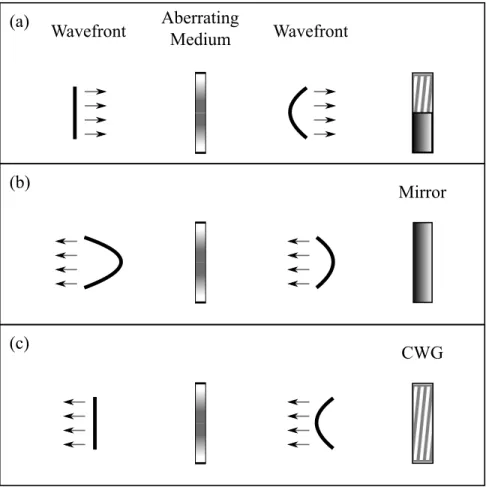
Figure 2.1.: Reflection vs. Conjugate Wave Generation: Wavefronts. (a) An incoming wavefront undergoes aberration. (b) The reflected wavefront is further deformed by a second pass through the aberrating medium. (c) The conjugate wavefront has its initial deformation corrected by a second pass.
of CWG are aberration correction schemes, in which optical wavefront aberrations caused by a medium of inhomogeneous refractive index are reversed in the conjugate wavefronts by a second pass through the same medium. The CWG mechanism usually takes the form of a so-called phase conjugate mirror, though the process is more akin to holography and diffraction than reflection. The effective differences between CWG and regular reflection are illustrated in Figures 2.1, 2.2 and 2.3.
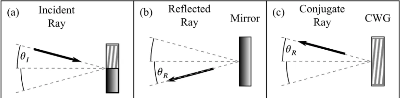
Mirror CWG 𝜃𝐼 Incident Ray 𝜃𝑅 Reflected Ray Conjugate Ray 𝜃𝑅 (a) (b) (c)
Figure 2.2.: Reflection vs. Conjugate Wave Generation: Ray Angles. Rays incident on a mirror at angle 𝜃𝐼 reflect at angle𝜃𝑅 = 𝜃𝐼, as in (b). CWG, by contrast, retro-propagates a ray such that𝜃𝑅 = 𝜃𝐼, as in (c), by the usual definitions of such angles. Partial Reflection Incident Ray CWG Pump (a) (b) Probe Signal
Figure 2.3.: Reflection vs. Conjugate Wave Generation: Powers. Power in the 'reflected' beam from a conjugate mirror is derived from one or more pump beams in a CWG system (b), not from the incident beam as in regular reflection (a).
The most useful property of CWG for most applications is the wavefront conjugation as illustrated in Figure 2.1, and expressed mathematically by Equation 2.1:
𝐄𝑠(𝐫, 𝑡) = 𝐀𝑠(𝐫)𝑒𝑖(𝐤⋅𝐫−𝜔𝑡) = 𝑟𝐀∗𝑠(𝐫)𝑒−𝑖(𝐤⋅𝐫−𝜔𝑡) = 𝑟𝐄∗𝑝(𝐫, 𝑡) (2.1) 𝑠, 𝑝 ⟹ Signal, Probe beams, resp.
𝑟 ≡'Reflectivity' coefficient of the CWG process 𝐀 ≡Amplitude of𝐄(including polarization)
𝐤 ≡Wave-vector
Complex conjugation of the probe beam's 𝐄𝑝 describes an exact reversal of its phase factor, indicating that the signal beam,𝐄𝑠, propagates as a time-reversed copy. The coefficient𝑟 accounts for the difference in power between the two beams. While𝑟 ≪ 1 is typical,𝑟 > 1is possible since the signal beam's power is not derived from the probe beam. It is this reflectivity coefficient that is measured, as a function of probe beam angle of incidence, in the experiment described in this dissertation. The CWG method used is known as Degenerate Four Wave Mixing.
2.1.2. DFWM
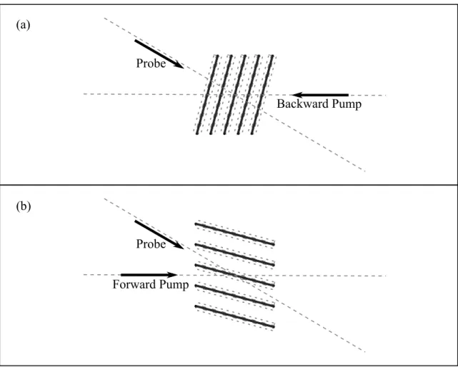
Degenerate Four Wave Mixing (DFWM) is a nonlinear optical process whereby a conjugate wave beam is generated at the intersection of three input beams within an optically nonlinear medium. Interference among the incident wave trains creates a periodic intensity pattern within the intersection region, which, given sufficient power, induce a similar pattern of nonlinear response within the target medium. The effect in an alkali vapor is that input beam pairs generate bands of greater and less refractive index, which act as diffraction gratings for the third beam. This effect is inversely proportional to the mean velocity of the atoms, as atomic drift blurs the periodic patterns, reducing grating effectiveness as illustrated in 2.4.
Backward Pump Probe Forward Pump Probe (a) (b)
Figure 2.4.: Index of Refraction Grating Patterns. The pattern (a) formed by the Probe and Backward Pump beams is less well defined than that formed by the Probe and Forward Pump beams (b).
2.1.3. Dependence of DFWM Efficiency on Beam Intersection Angle
Figure 2.4 illustrates not only the mechanism of DFWM, but also the effect of changes in pump/probe beam intersection angle. Two gratings are formed within the medium simulta-neously: one by the interaction of the Backward Pump and Probe beams, and another by the interaction of the Forward Pump and Probe beams. The spacing between grating planes becomes less as the angle between the interacting beams increases. This reduction in plane separation reduces the contrast of the grating, and therefore also the efficiency of the DFWM process. The Backward/Probe beam grating is, in fact, so ineffective that it contributes only negligibly to the DFWM process.
The geometry of the beams and grating is expressed mathematically by treating the grating itself as a wave, with a wave vector𝑘𝐺 = 2𝜋𝑠𝑖𝑛(𝜃/2)/𝜆, where𝜃is the beam intersection angle, and𝜆is the laser frequency [10]. For reference, the maximum angle at which the author ever observed measurable signal was approximately 220 mrad.
2.1.4. Role of Rb Diffusion and the Buffer Gas
High𝑘𝐺gratings have low contrast because of mixing atoms from optically saturated and unsaturated regions. At any instant of time, atoms in optically high intensity bands will become excited (assuming a simple, 2-level model), while those in low intensity bands will remain in the ground state. Thermal motion of the atoms causes mixing of these two populations, with the extent of the incursion of excited-state atoms into low intensity bands limited by the exited state lifetime (approx. 27 ns for the Rb D Line transitions) [17]. The diffraction gratings, therefore, maintain higher efficiency vs beam angle as the distance an excited Rb atom can travel in 27 ns is reduced.
The most likely means for limiting atomic travel is to operate at low temperatures. However, temperatures below 120∘result in too little gaseous Rb to be effective (see 2.5). A second mechanism for limiting atomic travel is to introduce what is known as a buffer gas, i.e. a second, nonreactive atomic species within which the primary species is made to
Figure 2.5.: Density and Pressure of Rb vs Temperature from [16]
diffuse. Frequent collisions with atoms of the buffer gas reduce the average velocity of the Rb atoms, and therefore also the mixing between the optically saturated and unsaturated populations.
In addition to collisional damping of the Rb thermal motion, light-weight buffer gases, such as the Helium used in the experiment discussed here, provide another mechanism for preserving the contrast of the gratings. A process known as quenching may occur at each collision between a He and an excited Rb atoms, wherein some of the energy lost by the Rb is taken from the atom's electronic configuration, resulting in a ground-state Rb post-collision. Thus, presence of a light buffer gas provides an effect that depends entirely on the frequency of collisions involving Rb atoms in the excited state, providing, ultimately, a macroscopic effect correlated to the Rb collisional cross section. An equation describing the magnitude of this effect is given by Glassner [10] as:
𝜌(2)2 − 𝜌(2)1 ∝ 1
𝐴21+ 𝐷2𝑘2𝐺{1 + 𝐷2 𝐷1}
𝐴21 ≡Einstein decay coefficient
𝐷2 ≡Excited-state diffusion coefficient 𝑘𝐺 ≡grating wave vector
The quantity𝜌(2)2 − 𝜌(2)1 in equation 2.2 is the difference in Rb population densities between the excited and ground states that creates the 3-dimensional grating pattern in the gas. The superscripts refer to a second-order polarization response of the Rb alkali atoms to the optical field. Full explorations of the relationship between CWG and nonlinear optics (i.e. effects in the 2nd and higher order terms of the electric fields) may be found in [5, 8].
2.2. Original Application
This section will describe the MDRb experiment as it was originally pursued. Central to calculations is the observation that the reflectivity𝑅 of the CWG process is directly proportional to the difference𝜌(2)2 − 𝜌(2)1 between the ground and excited state populations densities of the Rb sample. A useful modification of equation 2.2 is:
𝑅 = 𝑆 × 1
𝐴21+ 𝐷2𝑘2𝐺 {1 + 𝐷2 𝐷1} ,
(2.3) where𝑆is simply a scaling factor to allow for the overall magnitude of the response, and the control variable𝜃is present in the definition of the grating wave vector𝑘𝐺. Given that 𝑅is defined as the ratio between the powers of the signal (𝑃𝑆) and probe (𝑃𝑝) beams, and that the power of all input beams is to be held constant during throughout the experiment, a further refinement of equation 2.3 is:
𝑃𝑆 = 𝑆 × 𝐴 1
21+ 𝐷2𝑘2𝐺 {1 + 𝐷2 𝐷1} ,
(2.4) Equation 2.4 is lacking, notably, any reference to the frequency of the optical fields
(laser beams) used. This is because the measurement implied by equation 2.4 must use an optical frequency on resonance with specific electronic transition (in this case, the transition from52𝑆1/2to either52𝑃1/2or52𝑃3/2), with only the𝐴21parameter of the equation affected by the transition choice. In applied terms, the laser used must be frequency-locked to an atomic reference.
Given equation 2.4, the chain of measurements (from end to beginning) to be per-formed was:
1. Calculate the linear relationship between Rb𝐷2and1/𝑃𝐻𝑒via least squares fit to [𝐷2, 𝑃𝐻𝑒] data pairs.
2. Calculate value of𝐷2(𝑃𝐻𝑒)from least squares fits of equation 2.4 to [𝑃𝑆,𝜃] data pairs. 3. Measure𝑃𝑆values directly from an apparatus that implements CWG in a Rb/He gas
mixture at the specified𝑃𝐻𝑒and𝜃values.
2.3. Modified Application
Work on the MDRb experiment was successful in solving most of the technical challenges presented by the measurement, a discussion of which may be found in A. However, a funda-mental flaw of the measurement principle emerged along the way regarding the frequency of the laser radiation used and the Rb atomic transition to be utilized.
The original formulation of the experiment presupposed that a single transition could be excited (and saturated) within the Rb gas at a time, perhaps allowing, with the tunable diode laser available, two separate measurements (targeting the52𝑆1/2 → 52𝑃1/2 or52𝑆1/2 → 52𝑃3/2transitions) for each of the Rb isotopes (Rb85 and Rb87) present in the Rb/He gas cells available.
A B C D
Figure 2.6.: Simple Absorption and CWG Signal Power Profiles
2.3.1. Indistinguishably of Rb D-Line CWG Responses
The impossibility of the originally proposed measurement can be illustrated by figure 2.6; the upper oscilloscope trace is of a swept-frequency absorption profile in Rb (natural isotopic abundance of 72%/28% Rb85/Rb87) at room temperature. The Rb/He gas cells used in the experiment were heated to temperatures of∼ 130∘C in order to provide enough Rb vapor density to generate measurable signals, and the bottom trace in the figure is of the CWG signal power measured over the same range of laser frequencies. Obviously, the signal profile presents as a complicated mixture of atomic responses, allowing no straightforward separation of individual contributions.
2.3.2. Modification of Experiment Goals
Having found the originally conceived measurement to be unworkable, it was decided to attempt a different measurement with the measurement system as it stood; i.e., to adapt the measurement to the apparatus on hand. The new measurement target was taken to be a cumulative CWG reflectivity over the entire range of effective optical frequencies. The key equation for the new measurement was to be:
∫ 𝜔𝑏 𝜔𝑎 𝑃𝑆d𝜔 = 𝑆 ×𝐴 1 21+ 𝐷2𝑘2𝐺[1 + 𝐷2 𝐷1] , (2.5) where𝜔𝑎 and 𝜔𝑏were to be optical frequencies bracketing the entire D-Line interaction region for Rb at the temperatures required by the experiment (essentially everything shown in figure 2.6). It should be noted here that the value of∫𝜔𝑏
𝜔𝑎 𝑅d𝜔(hereafter denoted simply Σ𝑅, or Σ𝑃𝑆, depending on context) did not have any particular significance beyond its measurability, a fact that will be discussed further in 2.3.4.
The new chain of measurements was to be as follows (given in reverse order):
1. Accumulate [𝐷2,𝑃𝐻𝑒] measured value pairs (with𝐷2undefined), and see if a linear pattern exists between𝐷2and1/𝑃𝐻𝑒, as with the original experiment.
2. Calculate the𝐷2values from least squares fits of equation 2.5 to pairs of sets of [Σ𝑃𝑆, 𝜃] measured value pairs.
3. Calculate values forΣ𝑃𝑆(at specified𝜃configurations) from accumulated measure-ments of𝑃𝑆over a specific range of laser frequencies (a "frequency sweep").
2.3.3. New Experiment Requirements
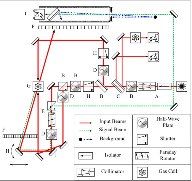
The need to vary the laser frequency during measurements imposed several extra require-ments on the experiment. As measurerequire-ments of reflectivity took the form of response profiles over a fixed frequency range, it was necessary to ensure that all such measurements were taken over the same frequency range. To this end, one of the two beam samples from the point labeled (C) in the figure 2.7 (this figure is more fully explained in A) was passed through a cell containing the same Rb mixture as the test cells, giving a resonance absorbtion profile at the associated photodiode. This and all other measured profiles were recorded synchronously with the ramped sweep of the laser frequency. The first step in the signal processing routine was then to use the features of the absorption profile to identify a central
A B B B C D D D E F F G H H I Half-Wave Plate Faraday Rotator B H J Gas Cell Collimator Isolator Background Signal Beam Input Beams Shutter
Figure 2.7.: Full Optics Assembly.
point along the frequency axis for that acquisition, and trim all of the acquired profiles to a set range about that point.
The second beam sample at point (C) is reflected directly into a photodiode, and monitors the laser power vs. frequency profile at that point. Departures from a flat power/fre-quency profile presented a problem as there was no way to distinguish between fluctuations signal strength due to changing reflectivity and those due to changes in strength of any of the input beams. In order to make accurate comparisons between signal profiles, it was necessary to normalize each signal profile by the power profiles of the input beams,
potentially requiring measured power profiles of each of the three input beams for every measurement. In the end, it was found that a series of careful alignment 'hacks' made it possible to reduce distortions in power/frequency profile to negligible levels between the point (C) and the cell at (G). In particular, optics designed for operation at near-normal beam incidence were avoided wherever possible, and even the cubes and wave-plates were aligned as far off of normal incidence as possible. In this way, and with some calibration, the three input beam power profiles could be kept equal and proportional to that of the sample at (C), save for effects caused by the target cell windows at (G). Etaloning at the cell windows was averaged out over multiple acquisitions at each beam intersection angle by slightly changing the cell pitch angle between measurements. This procedure simultaneously averaged out the interference fringes caused by input beam scatter from the cell at the signal measuring photodiode.
Most of the additional functional requirements entailed electronic and computerized interfacing. Design and implementation of these layers of the experiment was still underway when work was ceased. A partial list of the major requirements at the electronic/computerized level was:
• Simultaneous Analog to Digital Converstion (ADC) of all photodiode inputs (including digital storage of data streams) in synchrony with programmable modulation of the driving laser's output frequency (frequency ramp)
• Post-processing of the acquired photodiode waveforms to all data coming from the same span of optical frequencies (in effect, ensuring the repeatability of𝜔𝑎and𝜔𝑏) • Precise, motorized control, and automatic adjustment of the gas cell's pitch angle • Real-time calculation of the results of measurements over successive cell pitch angles • Automated control of the on/off state of the individual beams used to drive the CWG
• Simulation of the laser beam intersection geometry and intensity (in order to account for the effects of varying𝜃)
2.3.4. The Decision to Abort
Several years of work, on and off, were devoted to development of the MDRb experiment, culminating in a final year where MDRb became the focal pursuit within the laboratory. No single, insurmountable challenge ever arose, but neither did any end to the particular challenges encountered in the way of affecting a truly precise measurement. Ultimately, a review of the trajectory of the entire MBRb endeavor was made, and a decision reached that the modified experimental goal (Σ𝑅) was not valuable enough to warrant the resources being expended in its pursuit. Along the way, an investigation was begun into alternative approaches to the MDRb experiment that might have, at the least, allowed for quicker and more reliable identification of difficulties at the conceptual level of design, thereby lowering the effective cost (cost in time, if nothing else), of such endeavors in the future. It was discovered that the field known as Systems Engineering specifically offers methods and tools for the organized development and organization of knowledge about complicated systems. The remainder of this dissertation presents the results of an exploration of those methods as they might have been applied to the MDRb experiment.
CHAPTER 3
APPLICATION OF MODEL-BASED SYSTEMS ENGINEERING
The scope of this dissertation permits only a brief introduction to Model-Based Systems Engineering (MBSE), and to the modeling language known Systems Modeling Language (SysML). Readers interested in further reading will find plentiful introductory material on the internet, with the following resources being likely starting points:
• For SE and MBSE, the International Consortium on Systems Engineering (INCOSE) maintains a website with several introductory articles.
• For SysML (and the language UML on which it is based), the Object Management Group, which develops and maintains the official specification of those languages, maintains a website which provides both introductory materials and the formal speci-fication documents themselves.
3.1. MBSE
Systems Engineering (SE) is an approximately 100 year old discipline with roots in work done at Bell Laboratories in the 1930s [1, p. 8] The International Consortium On Systems Engineering defines SE, broadly speaking, as follows:
Systems Engineering is an interdisciplinary approach and means to enable the realization of successful systems. It focuses on defining customer needs and re-quired functionality early in the development cycle, documenting requirements, then proceeding with design synthesis and system validation while considering the complete problem....
Systems Engineering integrates all the disciplines and specialty groups into a team effort forming a structured development process that proceeds from concept to production to operation. Systems Engineering considers both the
business and the technical needs of all customers with the goal of providing a quality product that meets the user needs. [13]
Similarly from another source:
Systems engineering is a discipline that concentrates on the design and applica-tion of the whole (system) as distinct from the parts. It involves looking at a problem in its entirety, taking into account all the facets and all the variables and relating the social to the technical aspect. [2]
Increasing available of computers in the 1990s allowed SE practice to evolve from heavy dependence on paper documents to the use of single, large databases that contained information specified about the system under design, with human-readable diagrams acting as both views of, and handles on, the database. In other words, the goal of SE became increasingly a matter of producing and refining a unified model of the system in question, leading to the term "Model-Based" Systems Engineering.
The interdisciplinary nature of SE was one substantial reason for considering its application to experiments such as MDRb, which require the knitting together of diverse specialties such optics theory, optical engineering, electronics engineering, signal processing, software engineering, and measurement theory, all within a larger context of the need to serve the interests of both the larger scientific community, and the more immediate interests of those parties directly involved in the experiment's execution. The fact that MBSE was designed to provide an organized development from precise consideration of overall goals down to the detailed application of the diverse technical aspects of a system was also important, given the failure, in the case of MDRb, to fully specify the primary goal of the experiment before committing substantial resources.
The field of tools and practices called MBSE is fairly broad, and the decision to explore the application of MBSE was only the first of several needed to specify an overall
method to be investigated. Below is a brief account of several further specifying decisions that were necessary along the way:
3.1.1. Modeling Language
The options considered for modeling language were Archimate, the Object Process Method-olgy (OPM) language, and SysML. SysML was chosen in part due to the availability of documentation on its usage [6, 9], and also its inbuilt potential for handling mathematical relationships among the conceptual components of its model. SysML was derived directly from software engineering's Universal Modeling Language (UML), and inherited much of that languages capacity for precise capture of technical details.
Archimate is, technically, a language for work with Enterprise Architecture (EA), which is a variant of SE focused business and information technology systems, but encom-passing a domain of interests that has recently expanded to the engineering of physical assets [12]. While Archimate was not investigated in any depth for this work, it is the author's opinion that it may be a preferable language for modeling the "big picture" aspects of labo-ratory experiments, which may be, to some extent, viewed as a business venture intended to provide test results to interested parties (funding agencies, professional communities, etc.).
The language of OPM (which denotes both a language and a modeling method), while not as widely used, was considered both for reasons of its remarkable simplicity (the fundamental model elements are simply objects and methods), and for the fact that its creator, Dov Dori, seems to have had applications to the natural sciences in minds as he developed the language. In a recent book the subject, Dori makes observations that directly parallel those made during the review of work on the MDRb experiment:
...science can be thought of as reverse engineering of nature. When a system is being designed (by engineers) or investigated (by scientists), details about it accumulate quickly. The collected facts, be they real, assumed, contemplated or conjectured, become so voluminous that they are hard to master without an
orderly way of making sense of what is being revealed. Managing these facts is mandatory in order for them to make sense as a whole. In view of the rapid development of systems’ complexities, the need for an intuitive yet formal way of documenting designs of new systems or collected information about existing ones becomes ever more apparent. This, in turn, requires a solid infrastructure for recording, storing, organizing, querying, and presenting the knowledge being accumulated and the creative ideas that build on this knowledge. [7]
3.1.2. Questions of Framework and Methodology
In SE terminology, a Framework is a standardized set of modeling artifacts (diagrams, docu-ments, data files, etc.) to be produced during a given modeling effort. An SE Methodology is, similarly, a standardized set of modeling activities to be performed in a certain order during the modeling process. At the time of this writing, notable SE Frameworks in existence include The Open Group Architecture Framework (TOGAF), the Department of Defense Architecture Framework (DoDAF) and its equivalents in other countries, and the newly developed Unified Architecture Framework, which is intended to replace and unify DoDAF and its foreign counterparts. Methodologies include IBM's Rational Unified Process, and INCOSE's Object Oriented Systems Engineering Methodology (OOSEM) [9].
It was found, during the investigation of frameworks and methodologies for this work, that the investment required to learn to rigorously apply them was not warranted by the scope of the current project, and was, furthermore, perhaps inappropriate given the project's exploratory nature. Ultimately, a loose adherence to the OOSEM method proved practical, with a general flow of modeling focus from specification of stakeholders and their concerns (discussed in later sections), through requirements analysis, and logical/functional decomposition.
3.1.3. Software Tools
MBSE requires a specialized software environment, and a number of the currently available UML/SysML capable software tools were tested:
• MagicDraw, by No Magic
• Enterprise Architect, by Sparx Systems • Rational Rhapsody, by IBM
• Visual Paradigm
• Papyrus, which is an extension of the open-source Eclipse IDE
MagicDraw was used for the portion of the project concerned with modeling stake-holders/concerns (examples of the resulting diagrams are shown in the relevant section below). While MagicDraw proved to be a well-developed software, its high price made licensing unsustainable. Ultimately, the open-source Papyrus software was used for the majority of the modeling project. While not quite as polished and user-friendly as some of the other offerings, free availability and ongoing development made Papyrus a likely candidate for long-term use. Examples of Papyrus diagrams are shown in the 3.7 of this dissertation.
3.2. Modeling the Experiment as an Enterprise
The first phase of the modeling effort attempts to render the most significant features of the context within which the experiment exists. This is an example of Enterprise Systems Engineering, which is distinguished from Traditional Systems Engineering (or just Systems Engineering) by its emphasis on human factors and business processes. The goals at this stage of the modeling effort are to (a) establish clear terms and definitions, (b) provide top-level model elements for later use, (c) explicitly account for enterprise stakeholders and their concerns and, (d) establish clear requirements for subsystem architecture.
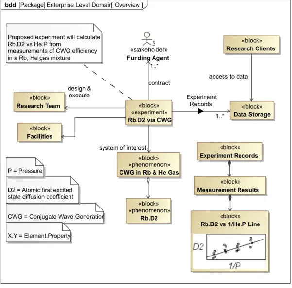
Enterprise Level Domain [Package] Overview bdd [ ] Rb.D2 vs 1/He.P Line «block» «block» Measurement Results Experiment Records «block» CWG in Rb & He Gas «block» «phenomenon» «block» Research Clients Research Team «block» Funding Agent «stakeholder» «block» «experiment» Rb.D2 via CWG Rb.D2 «block» «phenomenon» Facilities «block» Data Storage «block»
CWG = Conjugate Wave Generation Proposed experiment will calculate Rb.D2 vs He.P from
measurements of CWG efficiency in a Rb, He gas mixture
D2 = Atomic first excited state diffusion coefficient
X.Y = Element.Property P = Pressure design & execute Experiment Records 1..* access to data contract 1..* system of interest
Figure 3.1.: Overview of the Experiment in Context
3.3. Domain Level Overview
The Block Definition diagram (bdd) in figure 3.1 is drawn first (and subsequently refined) as a way of showing what is known as a black-box view (i.e., ignoring internal features) of the experiment within its larger context. This diagram is a kind of "conversation starter", and is intended to facilitate common understanding about the major features of the modeled enterprise, i.e. to answer the question "What, in general, are we talking about?". Further, elements added to this diagram on the first draft automatically become the first elements of the model.
As figure 3.1 is the first bdd presented in this dissertation, a detailed description is provided to explain the technical details. The central block Rb.D2 via CWG is of user-defined stereotype <<experiment>>. The tailless arrows in the diagram indicate associations, which are generic relations between model elements, the details of which are specified by embellishments on or near the arrow symbol. The block Research Clients is associated with Data Storage by a relation characterized by access to data. Taken clockwise, the experiment has associations with:
• Facilities, with no further details given
• a Research Team, where the text "design & execute" at one end of the arrow indicated the role Research Team fulfills in this context
• one or more (1..*) instances of Funding Agent, where the text "contract" in the middle of the arrow gives a name to the association itself
• one or more instances of Data Storage, where the filled arrowhead in the middle of the arrow line indicates that items named "Experiment Records" will be passed in some way in this direction
• a <<phenomenon>> named CWG in Rb & He Gas, which is the "system of interest" with respect to the experiment
Arrows with diamonds at the tail end indicate a special association known as com-position, which is a part-whole relation. The block Experiment Records is composed of other elements, among which is an instance of Measurement Results. A similar relationship exists between the two <<phenomenon>> elements. The filled diamond symbol indicates what is technically known as a Part Association, while the open diamond specifies a Shared Association [3, p. 38]. The distinction between these two concepts is sometimes character-ized as simply strong (Part) and weak (Shared) composition, with the latter meaning that the composing element can simultaneously participate in several such relations with multiple composites.
The rectangular symbols resembling dog-eared sheets of paper are instances of the SysML element <<comment>>, and serve only as a means to record text statements as model elements. The topmost comment is included in order to elucidate the significance of the experiment block, and space constraints force contracted names to be used for the elements themselves. The set of comments near the bottom are members of the model Glossary, which is simply a package containing comment elements for each such definition of terminology.
3.4. Stakeholders and Concerns
After specifying the main features of interest of the enterprise domain, the next priority is to specify the enterprise stakeholders and their concerns. This stage of the process might be thought of as answering the question "Who cares, and why?". Accounting for stakeholder concerns early in the modeling process allows later efforts to be explicitly anchored to their original motivations. The SysML specification defines the element <<stakeholder>>, while each concern is modeled as a <<comment>> [3, p.21]. These two elements are related in the sense that stakeholder "has" one or more concerns, as reflected in the SysML by the attribute concernList owned by the stakeholder classifier.
Stakeholder modeling may begin with a simple collection of the names of all people, roles, and organizations that have some interest in the proposed enterprise. Adding these stakeholders to a diagram is optional, but does provide a convenient means of getting the stakeholder elements into the model, as shown in figure 3.2. Organizing the stakeholders into logical groups is also optional, and it is useful, initially, to forgo organization altogether during brainstorming. A single new diagram element can be seen in figure 3.2; the arrows with open, triangular heads indicate a relation known as a Generalization, which communicates that the element on the tail end of the arrow is a special case of the element at the head.
Alongside the Stakeholders diagram, a similar diagram for collection of stakeholder concerns may be created and populated. No attempt is made yet to explicitly connect particular concerns with stakeholders in the diagram for two reasons: (1) stakeholder-concern
Stakeholders Brainstorm Stakeholders package [ ] «stakeholder» Researcher referencing results Committee Member «stakeholder» Review Committee «block» Researcher doing similar work «stakeholder» «stakeholder» Facilities Manager Academic Client «stakeholder» Funding Agent «stakeholder» «stakeholder» Research Client «block» Research Team «stakeholder» Peer Reviewer Team Member «stakeholder» Lab Operator «stakeholder» «stakeholder» Lab Manager «stakeholder» Supplier «stakeholder» Contractor Collaborator «stakeholder» «stakeholder» I.T. Manager Author «stakeholder» P.I. «stakeholder» «stakeholder» University NSF «stakeholder» «stakeholder» Regulator 0..* 0..* 0..* 1..* 1..*
Stakeholder Concerns Concerns Brainstorm package [ ] Records accessible and usable Maximize reusable equipment Adequate, appropriate facilities provided Records as complete as possible Compensation for good/services Stay within budget
Ergonomics & Safety Adequate funding Data security Results as precise as possible Maximize professional development Methods should be transparent and well documented Authorship on published paper(s) Finish within contracted time Maximize coincidental discovery Meaningful results Access to Results of Measurement Measurement should be repeatable
Figure 3.3.: Results of Concerns Brainstorm
relationships are potentially many-to-many, and therefore difficult to diagram, and (2) as of SysML 1.4, no model element is defined to denote this particular relationship on a diagram. In any case, minimal formality at this stage facilitates free thinking.
With stakeholders and concerns captured in the model, stakeholder-concern relation-ships are most easily recorded in a spreadsheet, or similar two dimensional array format. The software tool used for this work (MagicDraw), provides matrix building tools that were used to generate the matrix in figure 3.4. From within the software environment, this matrix is interactive; it automatically pulls stakeholder and concern entries from the model, and allows the relationships (blue arrows) to be established with simple button clicks. The matrix
Stakeholders Research Team
Academic
Clien
t
Author P.I. Collabora
tor Contra ctor I.T. Man ager Lab Man ager Supplier Lab Operator Research Clients Peer Reviewe r Rese arche r doing similar work Rese arche r refe ren cing re... Funding Agents NSF Univer sity Committee Membe r Regula tor Facilities Mana ger concern Legend Stakeholder Concerns
Access to Results of Measurement Adequate funding
Adequate, appropriate facilities provided Authorship on published paper(s) Compensation for good/services Data security
Ergonomics & Safety Finish within contracted time Maximize coincidental discovery Maximize professional development Maximize reusable equipment Meaningful results
Measurement should be repeatable
Methods should be transparent and well documented Records accessible and usable
Records as complete as possible Results as precise as possible Stay within budget
7 4 13 1 1 3 2 1 4 4 6 5 5 5 4 2 3 5 3 2 1 1 2 1 3 3 7 7 4 1 2 3 1 4 1 2 5 2 2 4 3 1 2 2 4 2 1 1 2 2 4 3 7 4 2 7 4 2 3 3 3 1 2
Figure 3.4.: Allocation Matrix of Concerns to Stakeholders
presentation provides an opportunity to review the collection of stakeholders and concerns for completeness; a stakeholder not associated concerns (or visa versa) bears closer scrutiny, as indicates either a gap in, or an extraneous addition to, the model.
All further steps in the modeling processes can now explicitly trace back to the stakeholder concerns being addressed. Moreover, presentations of the model tailored to a particular stakeholder can be informed by the list of concerns associated with that stakeholder.
3.5. Enterprise Use Cases
In order to begin a functional analysis of the enterprise in question, a collection of model elements called use cases are collected and specified. The information to be captured at this stage is summarized in the official SysML specification as follows:
The use case diagram describes the usage of a system (subject) by its actors (environment) to achieve a goal, that is realized by the subject providing a set of services to selected actors. The use case can also be viewed as functionality and/or capabilities that are accomplished through the interaction between the subject and its actors. [3, p.141]
In figure 3.5, the subject is represented by Rb.D2 via CWG block, with the actors display around the periphery. Ovals on the diagram represent use cases, and fact that the symbols are positioned within the block boundary indicates that these use cases are uses of the system represented by the subject block. Solid lines indicate a generic relationship called anassociation; i.e. a Funding Agent is associated with the usage called Contract Experiment. Where possible, dependencies between use cases are shown withincluderelationships; i.e. the Research Measurement usage includes the Gather Literature usage. As is always the case in MBSE, a given diagram only displays a selected subset of the relevant model elements. If useful, an entire separate diagram could be built around the Propose Experiment use case, for example, that might specify the detailed associations between specific members of the research team, various funding agents, and associated use cases. Any new model elements thus specified would, along the way, be collected into the model database, and become available for future use.
Each use case stands as a top level activity within the overall enterprise, and as such, may be taken as a starting point for further modeling. The usual progression (always subject to modification) is to pick a use case, specify detailed requirements that fulfillment of that use case must satisfy (always tracing back to stakeholder concerns if possible), and then
analyze the use case into a set of activities and system components that will fulfill the use case while satisfying the stated requirements. The remainder of this dissertation will focus on specification of the use cases Perform the Measurement and Model the Phenomena of Interest. Interestingly, the former use case proves to be a fairly typical subject of traditional systems engineering, while the latter use case is fulfilled entirely by the construction of a SysML model.
3.6. Modeling the Natural System of Interest
Application of MBSE to the modeling of natural systems is not much discussed in the currently available literature. The prospect is hinted at by Dori as a possible application for his OPM [7, p. 75], and attempts to translate between SysML and Modelica [11] point in a similar direction. During work on the experiment described in this dissertation, it was observed that a conceptual model of the Natural System of Interest (NSoI) was inevitably constructed (no measurement is possible without one), but never existed as more than a fragmentary set of ideas in the minds of the researchers, presumed consistent, and related informally to a printed document kept around the lab. Specifically, the experiment to be performed was derived entirely from a lengthy thesis [10] describing a similar experiment performed on several other alkali metals (other than Rb).
Typically, any research project will involve (as hinted at in 3.5) an initial review of the literature, and synthesis of an overview of the collected contents of relevant sources. In physics, or any other math-heavy field, one result of the review process is often a network of key equations given with interconnecting logic/derivations. The networked nature of this result suggests a diagrammatic representation, and several possibilities for such an interpretation exist within the SysML language. The equations themselves (the nodes of the network), should almost certainly be modeled as SysML Constraint Blocks, which are defined in [3] as:
Experiment Use Cases Overview Enterprise Level Domain
[Package] uc [ ] «block» «experiment» Rb.D2 via CWG Research Measurement to be Performed Establish Records Database Gather/Catalog Literature Access Experiment Records Disseminate Results Perform the Measurement Model Phenomena of Interest Contract Experiment Propose Experiment Facilities Manager «stakeholder» Research Journal External Records Storage «block» Research Client «stakeholder» «block» Research Team «stakeholder» Funding Agent Facilities «block»
One ore more members of Research Team are associated with each shown use case, but those associations are not shown in this diagram.
model requires research «include» «include» «include» «include» «include» «include» «include»
Figure 3.6.: Exapmle Parametric Diagram from [3]
such as performance and reliability models with other SysML models. Con-straint blocks can be used to specify a network of conCon-straints that represent mathematical expressions such as F=m*a and a=dv/dt, which constrain the phys-ical properties of a system.... A constraint block includes the constraint, such as F=m*a, and the parameters of the constraint such as F, m, and a. Constraint blocks define generic forms of constraints that can be used in multiple contexts. For example, a definition for Newton’s Laws may be used to specify these constraints in many different contexts
It should be noted that, in SysML, an entire diagram type, the Parametric Diagram, is devoted to the graphing of instances of Constraint Blocks and the equalities between parameters by which such constraints may be linked together. A typical example of a Parametric Diagram is given by Friedenthal [9]:
Constraint Blocks are the obvious model element to use for any type of equation. However, the relationships portrayed in 3.6 are not those typically employed in a lengthy mathematical derivation. It would be difficult, for example, to capture the logic binding a
Figure 3.7.: SysML Specifications of Constraint Block and Block from [3]
differential equation to its solution(s) by such methods.
A Constraint Block is, in SysML, a straightforward specialization of the basic ele-ment Block, and therefore the two diagrams for inter-Block relationships, Block Definition Diagrams (BDDs) and Internal Block Diagrams (IBDs), may be used. The distinction BDDs and IBDs traces to SysML's roots in UML, and UML's roots in object-oriented programming. The SysML Block specification inherits directly from the UML Class (figure 3.7), and, in OOP, Classes manifest as Class Definitions, and Class-defined Objects. In SysML, this distinction translates into Blocks and Instances of Blocks. A BDD portrays the details and relationships among Blocks (the definitions), while an IBD portrays the relationships among Instances (objects). The relationships portrayed in a BDD are abstract relations between definitions such as inheritance, composition, and general association; while an IBD show relations between objects such as equalities and usages, as well as containment of some objects within others.
3.7. Modeling the Mathematical Logic
The Internal Block Diagram proved the best context within which to effectively reverse-engineer chains of mathematical logic, and is perhaps (with a little bending of the rules), suitable to any such graphing of interrelated equations. Several of the resulting IBDs are presented below (with the rest left to an Appendix), but first explanation must be given for
methodology choices evident in the finished product.
3.7.1. The Question of Diagram Size
While the UML and SysML specifications impose no strict limits on the size of diagrams, the prevailing practice is to limit diagrams to what may fit, readably, on a standard letter sized page, or perhaps even the somewhat smaller pages of a printed, bound document (as is the case here). UML has not, to date, proliferated to the point that most people will have UML viewing software (as compared, for instance, to the PDF standard). It is right to assume, therefore, that any document viewed by anyone other than the author will be viewed in document format.
However, the work that resulted in the diagrams of this section presented two com-pelling reasons for allowing, in at least some case, essentially unlimited diagram size. The first reason relates to workflow: the process of scanning over one or more lengthy documents in order to glean and correlate the mathematical assertions is, by its nature, a disjointed and nonlinear process. The unification of such a scatter of visual data into a single, continuous whole is a primary advantage offered by a diagrammatic rendering in the first place. It was observed that any concern given during this part of the modeling process to constraints on size or interconnectedness tended to counter the primary goal of continuity. And so, the primary diagram (figure 3.8) was allowed to grow without limit, until all parts of the derivation were captured.
A second reason for the use of large format diagrams relates to the intended audience. The purpose of the model is to facilitate the planning and execution of an experiment in a laboratory. The particular experiment used for this dissertation was actively pursued over the course of several years, and involved a team that ranged in number from 2 to 4 people. A large format printout of figure 3.8 would have facilitated group discussions of the theory behind the experiment, particularly with group members not permanent enough to have been privy to formative discussions had in their absence. An accessible printout on dissertation,
with markers/pens nearby, would also allow all team members to participate in the gradual modification and update of the diagram.
For purposes of this document, accommodation to a smaller format was made in two ways. First, the image of the oversized diagram is rendered in scalable vector format, allowing viewers of electronic copies to magnify the image without limit. Second, a series of piecewise diagrams have been constructed from the same model elements in 6x8 inch format.
3.7.2. Capturing the Equations
Currently, SysML does not specify any particular language for the specification of Constraints. Within a SysML model, a Constraint exists simply as a String value listed under the Constraint Properties of a Block. Furthermore, at this time, none of the SysML modeling tools provides for the rendering of anything other than ASCII text. This means that, while one certainly may go to the trouble entering mathematical equations as Constraint strings (in Latex, or MathML, etc.), nothing of any value is thereby gained. Most UML/SysML modeling tools do, however, allow images to be displayed as part of the diagram elements. In order maintain best efficiency in the process of capturing equations into the model, images (SVG) of the typeset equations were used instead of actual Constraint specifications. This adds nothing to the model database beyond a Constraint Block with a descriptive name, but gives an easily recognized display of the equations in the diagrams, with minimal effort. All of the diagrams of this section had their equations images copied and pasted directly from the thesis document in which they were originally specified. New formulas can similarly be displayed either by use of a Latex editor, or any of a number of online Latex to image interpreters.
3.7.3. References
It is likely not possible (or desirable) to attempt construction of a model that would entirely supplant the original sources. In the interest of most efficiently using diagram space within
the tight constraints of this document, the decision was made to simply insert references to sources (mostly to Glassner's Thesis) in brackets at the end of each Block title. In general, a more sustainable approach (an approach more typical of UML) would be to give each block a Property, called Reference, with a𝑡𝑦𝑝𝑒 = 𝑠𝑡𝑟𝑖𝑛𝑔. This Reference property could then be given an appropriate default value. Further gains in model efficiency and fidelity could be had from the creation of a custom Stereotype, perhaps called <<Quoted Equation>>, with the Reference Property already built in. This custom element could inherit directly from Constraint Block. This approach was, in fact, attempted for the work presented here, but a bug in the Papyrus software would not allow proper display of the resulting blocks.
3.7.4. Mathematical Derivation in IBD Diagrams
The diagrams presented here are all IBDs. Aside from some instances of nested containment (rendered in straightforward manner), the relationships between the various elements were modeled as exclusively either Usage or Derive relations. The UML specification defines these as follows:
A Usage is a Dependency in which one NamedElement requires another NamedElement (or set of NamedElements) for its full implementation or opera-tion. The Usage does not specify how the client uses the supplier other than the fact that the supplier is used by the definition or implementation of the client. [4, p. 38]
Specifies a derivation relationship among model elements that are usually, but not necessarily, of the same type. A derived dependency specifies that the client may be computed from the supplier. The mapping specifies the computation. The client may be implemented for design reasons, such as efficiency, even though it is logically redundant. [4, p. 678]
The source document from which the all of the equations in this section were taken ([10]), was, at the time of this writing, available only as a photocopy. That fact, along with the lack of any mathematical typesetting capacity in the available MBSE software, necessitated some thought be to methods by which equations could be captured in human-readable form, without burdening the entire process beyond practical limits. A simple bitmap capture from the document image proved the most straightforward solution. Future developments in modeling software will, hopefully, provide more effective methods. For this dissertation, effort was made to compensate for the source material's quality by rendering the images somewhat larger than otherwise necessary. All diagrams are in scalable vector format, and may be enlarged as needed if viewed electronically.
3.7.5. The Primary Overview Diagram
The diagram in figure 3.8 is the original diagram used to gather and organize the relevant mathematical logic from the 100 page source document. The terminal point, in the bottom-right corner, is the single equation linking the entire derivation to the actual measurement around which the experiment revolved. Scattered throughout are explanatory quotes from the source document, inserted as UML Comments, which are (by the UML specification) portrayed as dog-eared notes. A collection of Comments in the top-left corner serve as a glossary of acronyms and otherwise obscure terms.
3.7.6. Small Format Diagrams
Because the information in a SysML model exists in a database, and not just on a given diagram, it is relatively easy to render subsets of the same information in other configurations on other diagrams. For the purpose of this document, smaller diagrams have been created that render the same information as figure 3.8, but in 6x8 inch sections. The diagrams are given as much as possible in a linear order related to the logic of the overall derivation modeled.
«Block» Governing Equations
: CWG Matrix Element, w/ Maxwellian Velocity Distribution [GTsec 2.2.2]
: 3rd Order Matrix Element, ab, w/ motion, Approx [GTeq 2.49] : Integrage over Velocity
In the homogeneously broadened case, which is found when the alkali atoms are mixed with significant pressure of inert buffer gasses, [Condition], and it is then possible to take the terms with [Term] in the denominator out of the integral, leaving:..." [GTpg 33] : Frequency Dependence Substituion
: Atomic State Time Derivative w/ Motion [GTeq 2.46]
: H.B. Approx. Condition : 3rd Order Matrix Element, ab, w/ Motion, V-dependence [GTeq 2.48]
: Maxwell Velocity Distribution [GTeq 2.44]
: 3rd Order Matrix Element, ab, w/Motion
: H.B. Approx. Term "Using the above substituion and
dropping terms with 2ωin the denominator we find the velocity dependent analogue to be..." [GTpg 31]
: Polarization Density, wave 4, with atomic motion [GTeq 2.45] : Use Modified Time Derivative in Schrodinger Eq.
: Substitution for Velocity Dependence [GTeq 2.47]
: P.C. Population Difference [GTeq 5.1] : Classical Field Equations for CWG, Stationary Atoms [GTsec 2.1, 2.21]
: Polarization Component Equations : Polarization Density to affect wave 4 [GTeq 2.37]
: Polarization Components [GTeq.2.11]
: Field Equation for DFWM [GTeq 2.43]
: E-Field to Polarization Relation [GTeq 2.18] : Polarization by Optical Field [GTeq. 2.10]
: Substitute Polarization, Simplifying Approximations : Nonlinear Polarization Density [GTeq 2.36]
: Substitute Matrix Elements and Equate Like-Order Terms
: Expanded Definitions : Complex Electric Field [GTeq 2.27]
: Density Matrix Elements Expanded [GTeq 2.28] : 2L Density Matrix Elements for CWG, Stationary Atoms [GTsec 2.1, 2.21]
: Solutions of Atom/Optical Schrodinger : Atom in Optical Field bb [GTeq 2.24]
: Atom in Optical Field aa [GTeq 2.25]
: Atom in Optical Field ba [GTeq 2.26]
: Substitute Definitions and Equate Like-Order Terms
: Reduced Density Matrix Elements : Zero Field Solutions [GTeq 2.29]
: 3rd Order Matrix Element for ab [GTeq 2.35] : Atom in Optical Field Schrodinger's [GTeq 2.23]
: CWG Matrix Element, w/ Diffusion [GTsec 2.2.3]
: Solutions of Schrodinger w/ Diffusion : Diffusing Atom in Optical Field bb [GTeq 2.51]
: Diffusing Atom in Optical Field aa [GTeq 2.52]
: Diffusing Atom in Optical Field ba [GTeq 2.53] : Schrodinger's w/ Diffusion [GTeq 2.50]
: Reduced Density Matrix Elements (Diffusion) : 3rd Order Matrix Element, ab, w/ Diffusion [GTeq 2.57]
: Substitute Definitioins and Equate Like-Order Terms (Diffusion)
: 3rd Order Element, ab, Diffusion, affection PC wave [GTeq 2.58] "...where Da, Db, and Dba = Dab are the diffusion coefficients for the ground state, the excited state, and the coherence, respectively." [GTpg 34]
"The effect of the Laplacian operator in Eqs. 2.51-2.53 is to add a term of the form Dk² to each occurance of the term -i
ω in the previously derived expansion coeffieients." [GTpg 35]
"The variation in the generated beam as the input beam directions are changed will be contained in the term.... Writing out this term, I obtain, after eliminating factors with 2ωin their denominator..." [GTpg 36]
«Problem» The nature of this Dependency is unclear. "From Eq. 2.57, we can write the population difference that has the correct phose and spatial frequency to generate phase conjugatte beams as...the population d correct phase aand spatial frequency for DFWM...." [GTpg 98] : Density Matrix [GTeq 2.20]
: Dipole Operator [GTeq 2.22] "CWG" = Conjugate Wave Generation
"GTeq #" = Glassner Thesis Equation # "GTpg #" = Glassner Thesis Page # "GTsec #" = Glassner Thesis Section # "2L" = Two Level (approximate atomic model) NOTE: a,b refer to the ground and excited levels throughout
use use «Derive» «Derive» use use use use «Derive» use «Derive» use use «Derive» «Derive» «Derive» «Derive» use «Derive» use use use «Derive» use «Derive» use «Derive» use use use «Derive» «Derive» use use use
To begin, 3.9 is intended to communicate the major logical sections in which the derivation proceeds. Relationships are here drawn only up to the borders of the major elements, and are to be taken as follows (ordered from bottom to top):
• The equation for the Phase Conjugating Population Difference is Derived from one or more elements in the logical section on Conjugate Wave Generating Matrix Element with Diffusion (the derivation thereof)
• CWG Matrix Element, w/ Diffusion, has some of its elements Derived from elements 2-Level Density Matrix Elements for Conjugate Wave Generation in Stationary Atoms • In similar fashion, Conjugate Wave Generating Matrix Element with Maxwellian
Ve-locity Distribution Uses 2L Density Matrix Elements for CWG, Stationary Atoms, and Derives from Classical Field Equations for Conjugate Wave Generation in Stationary Atoms
• Classical Field Equations... uses 2L Density Matrix Elements...
The diagram 3.10 begins the derivation proper, by specifying how a modified form of the Schrodinger's Equation for Atoms in an Optical Field uses, and is used by other elements of the derivation. Note the additional line of text (in parenthesis) above the title of several of the Blocks. This is a namespace specification, and indicates, for instance, that the Schodinger's w/ Diffuision element is part of the containing Block CWG Matrix Element, w/ Diffusion. This extra level of specification is necessary in order to relate the smaller diagrams to the larger.
Next, figure 3.11 illustrates that the same formulation of Schrodinger's equation yields solutions that, in turn, becomes the basis for a process wherein the mathematical definitions of several parameters (in particular, the optical field) are substituted in. This process, in its turn, yields expanded formulas for the elements of the Density Matrix, in particular the formula for a third order𝜌𝑎𝑏, as shown in figure 3.12.
«Block» Governing Equations
: 2L Density Matrix Elements for CWG, Stationary Atoms [GTsec 2.1, 2....
: CWG Matrix Element, w/ Diffusion [GTsec 2.2.3]
: CWG Matrix Element, w/ Maxwellian Velocity Distribution [GTsec 2....
: Classical Field Equations for CWG, Stationary Atoms [GTsec 2.1, 2.21]
: P.C. Population Difference [GTeq 5.1] "GTpg #" = Glassner Thesis Page #
"GTeq #" = Glassner Thesis Equation #
"2L" = Two Level (approximate atomic model) NOTE: a,b refer to the ground and excited levels throughout
"CWG" = Conjugate Wave Generation
"GTsec #" = Glassner Thesis Section #
«Derive» «Derive» «Derive» use use use use «Derive» «Derive» «Derive»
«Block» Governing Equations
(CWG Matrix Element, w/ Diffusion [GTsec 2.2.3]) : Schrodinger's w/ Diffusion [GTeq 2.50] (CWG Matrix Element, w/ Maxwellian Velocity Distribution [GTsec 2.2.2])
: Use Modified Time Derivative in Schrodinger Eq. : Density Matrix [GTeq 2.20]
(2L Density Matrix Elements for CWG, Stationary Atoms [GTsec 2.1, 2.21]) : Atom in Optical Field Schrodinger's [GTeq 2.23]
«Derive» use use use «Derive» use
«Block» Governing Equations
(2L Density Matrix Elements for CWG, Stationary Atoms [GTsec 2.1, 2.21]) : Atom in Optical Field Schrodinger's [GTeq 2.23]
: Dipole Operator [GTeq 2.22]
(2L Density Matrix Elements for CWG, Stationary Atoms [GTsec 2.1, 2.21]) : Solutions of Atom/Optical Schrodinger
: Atom in Optical Field bb [GTeq 2.24]
: Atom in Optical Field aa [GTeq 2.25]
: Atom in Optical Field ba [GTeq 2.26]
(2L Density Matrix Elements for CWG, Stationary Atoms [GTsec 2.1, 2.21]) : Substitute Definitions and Equate Like-Order Terms «Derive» use use «Derive» use use
«Block» Governing Equations
(2L Density Matrix Elements for CWG, Stationary Atoms [GTsec 2.1, 2.21]) : Substitute Definitions and Equate Like-Order Terms
(CWG Matrix Element, w/ Maxwellian Velocity Distribution [GTsec 2.2.2]) : Frequency Dependence Substituion
(2L Density Matrix Elements for CWG, Stationary Atoms [GTsec 2.1, 2.21]) : Reduced Density Matrix Elements
: Zero Field Solutions [GTeq 2.29]
: 3rd Order Matrix Element for ab [GTeq 2.35]
(Classical Field Equations for CWG, Stationary Atoms [GTsec 2.1, 2.21]) : Substitute Matrix Elements and Equate Like-Order Terms use «Derive» use use use «Derive»
«Block» Governing Equations
: 3rd Order Matrix Element, ab, w/ Diffusion [GTeq 2.57]
: P.C. Population Difference [GTeq 5.1] «Problem»
The nature of this Dependency is unclear. "From Eq. 2.57, we can
write the population difference that has the correct phose and spatial frequency to generate phase conjugatte beams as...the population d correct phase aand spatial frequency for
DFWM...." [GTpg 98]
«Derive» «Derive»
![Figure 2.5.: Density and Pressure of Rb vs Temperature from [16]](https://thumb-us.123doks.com/thumbv2/123dok_us/10928204.2981684/16.918.320.650.117.440/figure-density-pressure-rb-vs-temperature.webp)