Institut d’Economie Industrielle (IDEI)– Manufacture des Tabacs
July, 2010
n° 630
“Iterative Regularization in
Nonparametric Instrumental
Regression”
Jan JOHANNES,
Sébastien VAN BELLEGEM
Iterative regularization
in nonparametric instrumental regression
∗Jan Johannes1 S´ebastien Van Bellegem2 Anne Vanhems3
July 16, 2010
Abstract
We consider the nonparametric regression model with an additive error that is cor-related with the explanatory variables. We suppose the existence of instrumental vari-ables that are considered in this model for the identification and the estimation of the regression function. The nonparametric estimation by instrumental variables is an ill-posed linear inverse problem with an unknown but estimable operator. We provide a new estimator of the regression function using an iterative regularization method (the Landweber-Fridman method). The optimal number of iterations and the convergence of the mean square error of the resulting estimator are derived under both mild and severe degrees of ill-posedness. A Monte-Carlo exercise shows the impact of some parameters on the estimator and concludes on the reasonable finite sample performance of the new estimator.
Keywords: Nonparametric estimation, Instrumental variable, Ill-posed inverse problem, It-erative method, Estimation by projection
JEL classifications: Primary C14; secondary C30
∗
This work was supported by the “Agence National de le Recherche” under contract ANR-09-JCJC-0124-01 and by the IAP research network nr P6/03 of the Belgian Government (Belgian Science Policy).
1Institut de statistique, biostatistique et sciences actuarielles (Belgium)
2Toulouse School of Economics (France) & Center for Operations Research and Econometrics (Belgium) 3Toulouse Business School & Toulouse School of Economics (France)
1
Introduction
The statistical inference in the nonparametric regression model Y =ϕ(Z) +ε
whereY is a real dependent variable,Z is a real multivariate explanatory random variable andϕis an unknown function, usually requires that the error termεis such thatE(ε|Z) = 0. A vast literature is now available about the estimation of the nonparametric function in this setting, under various regularity assumptions on ϕ. Less work is however available if the errorεis allowed to be correlated withZ, a situation that is frequently encountered in the empirical studies in human sciences.
A simple situation where this correlation appears is when omitted variables influence both Y and Z but are not included in the explanatory vector of the regression model. One famous example of this situation appears when Y is a measure of the income of some individuals and Z is a measure of their level of education. It is likely that other variables, such as a measure of the social ability or the intelligence, may be influencial on both the income and the level of education of the individuals. However, this variable is rarely observed or even difficult to measure, and it is thus omitted in the regression model. In consequence, the error term ε contains an information about the omitted variable, and therefore may depend on the observed explanatory variables. This example is discussed in more details in many econometrics textbooks [e.g. Wooldridge (2008)], see also the survey written by Angrist & Krueger (2001).
One conventional approach to accomodate this problem is to measure a set of new variablesW that are called “instrumental variables” and such thatE(ε|W) = 0. Taking the conditional expectation of the above regression model, the nonparametric function ϕnow appears to be the solution of
E(Y|W) =E(ϕ(Z)|W). (1.1)
The choice of appropriate instrumentsW is a delicate question in practice. The interested reader can find examples of instrumental variables in the above econometric references.
As a statistician, the interesting and nonstandard point is that the nonparametric func-tion ϕ appears to be the solution of an integral equation given by (1.1). It is thus the solution of an ill-posed inverse problem. Moreover, the involved conditional expectations must be estimated from observations of (Y, Z, W), which is a source of error in both sides of equation (1.1).
A number of papers have considered the estimation of ϕin model (1.1) from the obser-vation of (Y, Z, W) when the conditional expectations are estimated nonparametrically and by regularizing the ill-posed problem in order to recover a consistent solution. We refer to Hall & Horowitz (2005) for some methods and to our recent paper, Johannes et al. (2010),
that presents a unified approach to get consistent estimators of ϕ with optimal rates of convergence.
One goal of this paper is to present new results on a regularization scheme that has been less studied in this context. This regularization is the so-called “Landweber-Fridman” iterative procedure that we define below. Moreover, our estimator of the conditional ex-pectations and ϕ are projection estimators onto finite-dimensional vectorial spaces, with dimension increasing with the sample size. The expansion of the nonparametric functionϕ is provided in a basis that may be different from the basis that is used to estimate the condi-tional expectations. This aspect of our procedure is valuable, since the degree of regularity of ϕmay be very different from the degree of regularity ofE(ϕ(Z)|W).
Under a set of minimal conditions on the choice of those bases, we prove the consistency and the mean square convergence of the estimator given by iterative regularization. Results are given for both the mildly and severely ill-posed inverse problems, and reach the optimal minimax rate of convergence in standard function spaces in both cases. The results also give optimal stopping rule for the iterative regularization of the estimator.
The paper is organized as follows. In Section 2, we introduce the necessary notations of the paper and, more importantly, we formulate the estimation problem as an ill-posed inverse problem with an unknown linear operator. In Section 3 we derive the projection estimator and apply the regularization iterative method of Landweber-Fridman. Theoretical properties of the estimators have to be found in Sections 4 and 5. Those sections include the derivation of the rate of convergence under the various sets of regularity conditions, and provides a comparison with the most recent results of the literature. Section6discusses the role of the parameters in the estimation procedure and shows the finite sample properties of the proposed procedure via simulations. The proofs and technical results are deferred to an Appendix.
2
Model and assumptions
Let Z ∈ Rp and W ∈ Rq be two vectors of observed variables. In this section, we will write the nonparametric functionϕas a solution of an inverse problem. Define the function spaces L2Z ={φ:Rp →R,kφk2 Z :=E[φ2(Z)]<∞} and L2W ={ψ:Rq →R,kψk2 W :=E[ψ2(W)]<∞}.
For the sake of readability, we shall denote byh·,·iandk · kthe inner product and norm for both Hilbert spaces L2Z and L2W when there is no possible confusion about the functional space in question. The equation (1.1) can be rewritten
ifr is a function ofL2
W such thatr(·) :=E(Y|W =·) andT is a linear operator that maps
the functionϕonto the conditional expectation, i.e. T :L2Z→L2W :φ7→E(φ(Z)|W =·)
assuming the existence of the conditional density ofZ given W, here denoted by fZ|W. For convenience, we will assume in the following that the operator T is a compact operator. This assumption implies that T and the adjoint operator T⋆ can be discretized
using a singular value decomposition (SVD). We recall that the compacity ofT implies the existence of a singular system{(λk, uk, vk);k= 1,2, . . .}that is such that:
1. The eigenvalues λk are real, strictly positive and decreasing;
2. {λ2
k;k = 1,2, . . .} are the nonzero eigenvalues of the self-adjoint operators T⋆T and
T T⋆;
3. {uk;k = 1,2, . . .} (resp. {vk;k = 1,2, . . .}) is an orthonormal system of eigenvectors
of T⋆T (resp. T T⋆).
The existence and uniqueness of the solution from equation (2.1) needs some assump-tions. A detailed discussion on identification issues can be found in the seminal work of Darolles et al. (2002). In the sequel, we assume the existence and uniqueness of the solu-tion. Uniqueness is guaranteed if we assume the operator T to be injective. The existence assumption formally requires that the functionr belongs to the range of the operatorT.
From (2.1), we see thatϕcan be recovered by inverting the operatorT. However, even if T is in general an invertible operator, it is not necessary stable or, in more technical terms, T−1 is not a bounded operator. In other words, since the left hand side of equation (2.1) is
not observed directly but needs to be estimated by ˆr, the solutionT−1rˆdoes not converge to T−1r. That phenomenon is called the “ill-posedness” of the inversion. Therefore, in order to derive a consistent estimator of the functional parameter of interest ϕ, we shall proceed in two steps. First,T andr depend on the distribution of (X, Y, W) and are estimated from the dataset using projection method. Second, a regularized version of (2.1) is obtained using a Landweber-Fridman iterative method.
We now describe the two steps in detail.
3
Estimation and regularization
3.1 Projection step
Define two finite dimensional subsets ΦdZ of L
2
Z and ΨdW ofL
2
W. Their dimension depend
on prescribed numbers dZ, dW > 0 and we suppose that {φ1, . . . , φdZ} is a basis for ΦdZ
and {ψ1, . . . , ψdW} is a basis for ΨdW. Note that the each of these bases is not necessarily
The two bases are chosen independently of the operatorT. However, our theory requires a condition that relates both the bases and T. Denote by PZ, resp. QW, the orthogonal
projection onto ΦdZ, resp. ΨdW and by I the identity operator. We assume from now on
that the operatorsPZ, QW and T are such that
kT(I−PZ)k →0 and k(I−QW)Tk →0 (3.1)
as (dZ, dW)→ ∞, where the norms are the operator norm, e.g.
kTk:= sup{kT ψkW; ψ∈L2Z}
is the operator norm of T. This condition is discussed in the following remark and two examples.
Remark 3.1. Because Φd
Z and ΨdW are finite dimensional, the range of the operators PZ
and QW that we denote by R(PZ) and R(QW) are finite dimensional. Using a result to
be found in Plato & Vainikko (1990), a necessary and sufficient condition in order to get condition (3.1) is that (i) T is a compact operator, (ii) PZ → I pointwise on R(T⋆) as
dZ → ∞ and (iii)QW →I pointwise onR(T) as dW → ∞. In particular, it is not difficult
to derive from the singular value decomposition that the following two inequalities hold:
kT(I−PZ)k>λdZ
and
k(I−QW)Tk>λdW.
Therefore, whatever the two bases are, the best approximation ofT cannot perform better than the rate of the singular values λdZ and λdW. Note that the equality holds when the
bases are chosen to be the eigenfunctions {uk;k = 1, ..., dZ} and {vk;k = 1, ..., dW}, but
this situation is not useful in our context sinceT is unknown. Example 3.1. To simplify this example, assume that Z and W are uniformly distributed over [0,1]. Let s0, . . . , sdZ denote an equidistant grid on [a, b], that is sk = a+kτ with
τ = (b−a)/dZ. Define φk := I[sk−1,sk] for k = 1, . . . , dZ as a basis of ΦdZ. Analogously,
define a grid on [c, d] with tk = a+kτ with τ = (d−c)/dW and Ψk := I[tk−1,tk] for
k= 1, . . . , dW. For this example with a sufficiently smooth joint density fZW, we can write
(cf. Plato & Vainikko (1990))
kT(I−PZ)k6c1·(b−a)/dZ, c1= 2 3 Z b a Z d c ∂fZW∂z(z, w) 2dwdz1/2, k(I−QW)Tk6c2·(d−c)/dW, c2= 2 3 Z b a Z d c ∂fZW∂w(z, w) 2 dwdz1/2.
With additional regularity assumptions on fZW, it is useful to consider more regular
basis functions, such as higher order B-splines or wavelets for instance. This would lead, for example, to upper bound for kT(I −PZ)k of the type ((b−a)/dZ)η. The exact value
of η depends on the basis system and the smoothness of fZW and is derived from typical
inequalities in approximation theory (cf. DeVore & Lorentz (1993)). Example3.2. An interesting example for Φd
Zis given by the basis of orthonormal wavelets.
The theory of wavelets offers an appealing alternative to the Fourier analysis. A wavelet system is an orthogonal basis of L2(Rq) which, in contrast to the Fourier basis, contains
functions that are well localized both in the time and the frequency domain. As a conse-quence, they appear more appropriate to decompose functionsϕthat have a more irregular behavior, such as jumps or peaks. For a general introduction to this theory, we refer to Vidakovic (1999).
Suppose that Z and W are uniformly distributed over [0,1]. Let (φ, ψ) be some scaling and mother functions over [0,1] and assume that ψ has κ continuous derivatives and κ vanishing moments. Let j be a negative integer. The space ΦdZ in this example is the
linear space that is spanned by{φjk}06k<2−j−1, withφjk(·) := 2−j/2φ(2−j· −k). Denote by
Pj the orthogonal projection onto this space. For any functiong belonging to the Sobolev
space Ws[0,1] for 0 < s < κ, one can show k(I −P
j)gk2 = o(22sj) (e.g. Mallat (1997,
Theorem 9.4)). Therefore, some calcuation show that
kT(I−Pj)k6C22sj
Z
kf(·, w)/pr(w)k2Wsdz
provided that [f(·, w)/pr(w)] ∈Ws and that the integral exists. A similar bound can be
derived fork(I−Q)Tk.
We are now in position to describe the projection step of the estimation. Find a solution ϕ◦∈Φ
dZ of the system of equations
hT ϕ◦, ψji=hr, ψji for all j= 1. . . dW.
This system is a discretization of the problem (2.1). Since ϕ◦ ∈ ΦdZ, we can write ϕ
◦ =
PdZ
j=1a◦jφj which, by linearity of the operatorT, leads to the equivalent system of equations
˜
Mda◦= ˜vd (3.2)
wherea◦= (a◦
1, . . . , a◦dZ)
′is the vector of parameters, ˜M
dis thedW×dZmatrix with element
(i, j) equal to hT φi, ψji and ˜vd is the column vector (hr, ψ1i, . . . ,hr, ψdWi)
′. The inversion of the system (3.3) however leads to two important issues. The first issue is that the basis systems {φ1, . . . , φdZ} and {ψ1, . . . , ψdW} are not orthonormal. Thus the inversion of (3.3)
involves the Gram matrices Gφ:= (hφi, φji)i,j=1,...,dZ
and
Gψ := (hψi, ψji)i,j=1,...,dW.
These two matrices reduce to the identity matrix when the basis systems are orthonormal. With this correction, (3.2) becomes
Mda◦=vd (3.3)
whereMd=G−ψ1/2M˜dGφ−1/2 and vd=G−ψ1/2v˜d.
The second issue is the stability of the inversion. Because we are solving an integral equation, the problem (2.1) is in general ill-posed. This implies that the matrixMdin (3.3)
is ill-conditionned and thus its inversion is numerically unstable. In particular, it implies that, even if we find a consistent estimator for Md and vd, the estimation of a◦ resulting
from the inversion of (3.3) has a very slow rate of convergence in general. For this reason, we need to stabilize (regularize) the inversion in order to recover faster rates of convergence in the estimation of ϕ. Below we propose an iterative method for this issue. However, before presenting this method, we first introduce consistent estimators of Md and vd.
3.2 Estimation of Md and vd
Let{(Yl, Zl, Wl);l= 1,2, . . . , n}be an independent and identically distributed sample from
(Y, Z, W). Let φ(·) = (φ1(·), . . . , φdZ(·))
′ and ψ(·) = (ψ
1(·), . . . , ψdW(·))
′. The estimators of Mdand vd are respectively given by
c Md= 1 n n X l=1 G−φ1/2φ(Zl)ψ(Wl)′G−ψ1/2 (3.4a) and b vd= 1 n n X l=1 YlG−ψ1/2ψ(Wl). (3.4b)
We give below some asymptotic properties for these two estimators that will be useful to derive the final rates of convergence. The result is valid under the following assumption. Assumption 3.1. Denote φ˜ = G−1/2
φ φ and ψ˜ = G
−1/2
ψ ψ. The vectors φ˜ and ψ˜ are the
orthogonalization of φandψ by the Gram matrices. We assume: kφ˜ikζ
LζZ 6c·d (ζ/2)−1 Z and kψ˜ikζ LζW 6c·d (ζ/2)−1 W for all ζ >2.
It is not difficult to check that Assumption3.1holds true for the basis introduced in the two examples.
Proposition 3.1. The estimators Mcd, resp vbd, are unbiased for Md, resp. vd. Suppose that EY2 <∞. Then, under Assumption 3.1it holds1
Ekbvd−vdk22. dW n , (3.5) EkMcd−Mdkζ 2 . (dWdZ)ζ/2 nζ/2 for all ζ ∈(0,2], (3.6) EkMcd−Mdkζ 2 . (dWdZ)ζ−1 nζ/2 for allζ >2, (3.7)
where k · k2 is the ℓ2 norm of a matrix.
Proof. The unbiasedness of Mcd and bvd is a straightforward result. The proof of (3.5) is
similar to the proof of (3.6), therefore we skip it.
Application of Lyapunov’s inequality leads to EkMcd−Mdkζ
2 6 (EkMcd−Mdk22)ζ/2 for
all ζ ∈ (0,2]. Moreover, if Md;ij denotes the element (i, j) of the matrix Md, we have
EkMcd−Mdk22 6P
i,jVarMcd;ij because Mcd is an unbiased estimator of Md. Then we can
write, by independence of the sample, VarMcd;ij 6 1
nE{φ˜i(Z)
2ψ˜
j(W)2} (3.8)
This last expression is finite as the functions ψj, φi are such that kψ˜jkL2 W = k
˜ φikL2
Z = 1
for all i, j. The inequality (3.6) follows by noticing that the sum over i, j contains dWdZ
elements.
We now prove (3.7). Using Jensen’s inequality
EkMcd−Mdkζ 2 = (dWdZ)ζ/2E 1 dWdZ X i,j (Md;ij−Mcd;ij)2 ζ/2 6(dWdZ)(ζ/2)−1 X i,j E(Md;ij −Mcd;ij)ζ .
To simplify notations, write Mcd;ij = n−1PlAij;l where Aij;l := ˜φi(Zl) ˜ψj(Wl). By the
inequality of Minkowski, it holds E|P
iXi|p 6{Pi(E|Xi|p)2/p}p/2 and we can then write
E(Md;ij −Mcd;ij)ζ 6n−ζ{X l (E|Aij;l−EAij;l|ζ)2/ζ}ζ/2 .n−ζ{X l (EAζ ij;l)2/ζ}ζ/2 (3.9)
using again Jensen’s inequality. As above when we derived the upper bound of (3.8), we note that EAζ ij;l.kψ˜jk ζ LζW · k ˜ φikζ
LζZ. Therefore, with Assumption 3.1, (3.9) is bounded by
n−ζ/2(dZdW)(ζ/2)−1 and the result follows.
3.3 Regularization iterative step
We now present the iteration procedure used in order to stabilize the inversion of the system (3.3). It is called theLandweber-Fridman in the numerical literature [e.g. Engl et al. (2000)]. It is of course possible to define other regularization schemes at this stage, among which is Tikhonov regularization. The Landweber-Fridman has the advantage to be numerically very simple to implement when it is applied to the projection estimator.
The vector a◦ in the system (3.3) is estimated by the following way:
b a◦0 = 0 b a◦k+1=ba◦k− 1 µ2Mc ′ d c Mdˆa◦k−bvd k= 0,1, . . . , K−1 (3.10) The estimator ofϕ◦ then follows by
b
ϕ◦ :=ba◦′KG−φ1/2φ. (3.11)
The presence of the parameter µ in the iterative scheme is only technical. The con-vergence results established below need that the norm of the matrix used in the algorithm must be less than 1. The parameter µ then normalizes the problem such that this con-straint is fulfilled. In practice and in the proof of our results, we use the random bound µ >max(1,kMcdk).
One crucial question is to decide on the number of iterations K. It is known that a too small value ofK provides unsufficient regularization, whereas a too large value of K leads to a too large regularization bias. The theoretical sections below and the empirical study provide a guidance for the choice of this regularization parameter.
4
Convergence under mild ill-posedness
In order to derive a rate of convergence for our estimator we need to specify regularity assumptions for the unknown solutionϕ. One convenient approach is to relate the regularity of ϕ to the behavior of the operator T itself. The idea is that, if ϕ is well adapted to the operator, then the estimation should be easier, thus the rates of convergence should be faster. The meaning of how “well-adapted” is the solution to the operator is characterized by the so-calledsource condition that we define now.
The natural operator of interest in order to define our source condition is T⋆T, which
is by construction self-adjoint, non-negative and such that T⋆T g=X
k∈N
λ2khg, ukiuk for all g∈L2Z
by definition of the singular value decomposition of T.
In the following it is useful to define what is a function of T⋆T. Consider a function
decomposition: ℓ(T⋆T)g:=X k∈N ℓ(λ2k)hg, ukiuk (4.1) for all g∈L2 Z.
The regularity assumption imposed on the solution ϕis defined next.
Assumption 4.1 (Strong source condition). The operator T and the solution ϕ are such that there exists β >0 and ψ∈L2Z with ϕ= (T⋆T)β/2ψ and kψk6ρ.
To understand this condition it is convenient to note that it is equivalent to require that the solution ϕ is such that (T⋆T)−β/2ϕ belongs to L2
Z. Using the singular value
decomposition ofT and the representation given in (4.1) it is therefore equivalent to assume ∞
X
k=1
(hϕ, uki)2
λβk <∞.
Because the eigenvalues λβk tend to zero, the index β that appears in the source condition is one measure of the ill-posedness of the problem.
Before stating the convergence result, we also formalize the condition (3.1) on the op-erators PZ, QW andT in the following assumption.
Assumption4.2. The projection operators PZ, QW andT are such that kT(I−PZ)k6δZ and k(I −QW)Tk6δW, where δZ, resp. δW, denote two sequences vanishing as dZ, resp.
dW, growth.
Theorem 4.1. Consider the estimator (3.11) constructed using the projections PZ and QW and setµ=Cmax(1,kMˆdk)for some constant C >1. Suppose that the “strong source
condition” (Assumption 4.1) is satisfied, that EY2 <∞ and Assumptions 3.1and 4.2 hold true. Assume that the number of iterations K is such that
K= δZ2+2(1∧β)+dW(dZ+ 1) n −β+11 . (4.2)
Then the L2 risk of the proposed estimator ϕb◦ has the rate Ekϕˆ◦−ϕk2 =O dZdW n β β+1 +δ2(Zβ∧1)+δW2(β∧1) ! .
Proof. An upper bound for the mean square error of ϕb◦ under the strong source condition is derived in LemmaB.1 in the technical Appendix, and is given by
Ekϕˆ◦−ϕk2 .{1+EkMcd−Mdk2β 2 }K−β+K EkMcd−Mdk22+Ekbvd−vdk22+δ2+2(β∧1) Z +EkMcd−Mdk2(β∧1) 2 +EkMcd−Mdk22β+δ 2(β∧1) Z +δ 2(β∧1) W .
First we note that 1 +EkMcd−Mdk2β
2 .1 by Proposition3.1. We find the optimal number
of iterationsK by balancing the first two terms, which gives: K∼nEkMcd−Mdk2+Ekrbd−rdk2+δ2+2(β∧1)
Z
o−β+11 .
The above Proposition3.1gives the rate of convergence forEkMcd−Mdk2 and Ekbrd−rdk2, and they lead to the optimal rate (4.2) given in the statement of the theorem. We plug in the optimal rate for K in the MSE of ϕb◦, and we consider the leading terms we get
Ekϕˆ◦−ϕk2 . dZ(dW + 1) n β β+1 + dZdW n β∧1 +δ 2β(1+β∧1) β+1 Z +δ 2(β∧1) Z +δ 2(β∧1) W .
The result follows by considering the leading terms and using the inequalities β/(β+ 1)6 β∧16(1 +β∧1)β/(1 +β) that hold for allβ >0.
We comment this result in the following remarks.
Remark 4.1. 1. The result is presented under mild conditions on the bases used for the projection. Now impose m := dZ = dW and δZ = δW = m−4β. If β 6 1 then the
rate of convergence of the risk reduces to n −β
β+3/2 which is known to be optimal in
the class of solutions that satisfy the strong source condition [Johannes et al. (2010, Proposition 4.1 with s= 0,a= 1 and p=β)].
2. One interesting example is given when the projection basis is given by the singular value decomposition ofT. We have already argued that this case is not realistic since the eigenfunctions are unknown, but it is at least of a theoretical interest. From Remark 3.1 it follows that δZ =λdZ and δW = λdW. We may also impose that the
eigenvalues are decreasing at a polynomial rate, i.e. λd =d−ε for some ε >0. Then
the rate is given by n −2β
2β+2+1/ε. This particular setting has been considered for the
study of other regularization methods in Hall & Horowitz (2005). This rate is known to be optimal for mildly ill-posed inverse problems over the space of functionsϕthat satisfy the source condition [e.g. Chen & Reiß (2010)].
3. The discontinuity (β ∧1) on the range of the exponent of δZ and δW implies that
the rate is no longer optimal for β > 1. This limitation is not technical, but it is intrinsic to the Landweber-Fridman method (the mathematical explanation is given by the analogous limitation in Lemma B.1 in the Appendix below). A similar phe-nomenon has been observed in Tautenhahn (1996) in a purely deterministic setting. In Tautenhahn (1996) a so-called “preconditionning” treatment has been proposed to improve the rate whenβ >1. We conjecture that a similar solution would lead to the same improvement of our result.
5
Convergence under severe ill-posedness
There are a number of important situations where the strong source condition is a too restrictive assumption. A prominent example is given by random variablesZandW that are normally distributed. In that situation one can show that the eigenvalues of the conditional expectation operatorT are exponentially decreasing, i.e. λkbehaves like exp(−kε) for some
ε >0. Under this setting, the functions satisfying Assumption 4.1 for an arbitrary β > 0 would be very limitated. Indeed, Assumption 4.1 would imply that the solution ϕ has an infinite number of derivatives (i.e. ϕis an analytic function). This example show that the strong source condition may be restrictive.
We can define a weaker condition than Assumption4.1if we consider the functionℓin the representation (4.1) to be logarithmic. This case has been considered in the deterministic setting [e.g. Hohage (1997); Nair et al. (2005)]. Surprisingly, it has been less studied in the context where the function r and the operator T have to be estimated [see Chen & Reiß (2010) for a related condition].
Assumption 5.1 (Weak source condition). There exists ψ∈L2
Z such that ϕ= −log T⋆T 2 −β/2 ψ, kψk6ρ and β >0, (5.1) where ρ is sufficiently small.
Note that this assumption is well defined since T and T⋆ are conditional expectation operators and therefore they are projections and such that kT⋆Tk = 1. The following theorem gives the asymptotic risk under the weak source condition.
Theorem5.1. Consider the estimator (3.11) constructed using the projectionsPZ andQW and set µ=Cmax(1,kMˆdk) for some constant C >1. Suppose the weak source condition
(Assumption 5.1) is satisfied and dZ, dW are such that (dZdW)/n2 =O(1). Suppose that
EY2 <∞ and Assumptions 3.1and 4.2 hold true. If the stopping index K is chosen by K= dZdW n +δ 2 Z+δW2 −1/2 (5.2) then we have Ekϕˆ◦−ϕk2 . log dWdZ n +δ 2 Z+δ2W −β .
Proof. In Lemma C.1of the technical Appendix, we have derived the mean square error of
b
ϕ◦ under the weak source condition. This lemma together with LemmaA.2 gives
Ekϕˆ◦−ϕk2 .K{EkMcd−Mdk22+Ekbvd−vdk22+δZ2 +δW2 }+ 2(logK)−β (5.3) provided that K, dW anddZ are such that
Proposition 3.1 applied to the rate (5.3) leads to Ekϕˆ◦−ϕk2 . K{dZ(dW + 1)/n+δ2
Z+
δW2 }+ 2(logK)−β. With K such that (5.2) holds, and considering the main terms, then the mean square rate of convergence follows. It remains to check if the constraint (5.4) is fulfilled. The norm (5.4) can be decomposed into three terms:
K2EkM′M−Mc′ dMcdk22 .K2 n EkM′(M −Mc)k2 2+Ek(M′−Mcd′)(Mcd−Md)k22 +EkMd(M′−Mcd′)k22 o
Using Proposition 3.1, the first and the second term are bounded by K2(δ2
W + δZ2 +
(dWdZ)/n). Using the Cauchy-Schwarz inequality and Proposition 3.1 with ζ = 4, the
second term is bounded up to a constant by K2(δW2 +δZ2)(dWdZ)3/2/n+K2(dWdZ)3/n2.
Therefore, with the choice ofK given in (5.2), it is sufficient to satisfy the constraint
(dWdZ)3 n2 + dWndZ + (δW2 +δZ2) 1 +(dWdZ)3/2 n dZdW n +δZ2 +δ2W =O(1).
The last constraint is satisfied under the condition that (dWdZ)2/n is finite.
Remark 5.1. 1. The optimal number K of iterations found in this result appears to be independent from the β, that is it is independent from the level of regularity of ϕ given by the weak source condition.
2. Suppose we take the same number of basis functions m:= dW =dZ in both Hilbert
spaces. Suppose also that the basis is such that δZ = δW = exp(−m2ε) from some
positive number ε. Then if we take e.g. m = n1/4 the final rate of convergence is
{log(n)}−β. When T and r which are known and deterministic, this rate is known
to be the optimal rate of convergence over the solutions that satisfy the weak source condition [Hohage (2000)].
6
Finite sample study
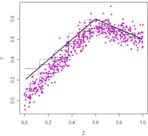
We present here the results of a Monte-Carlo study that aims to study the finite sample properties of the suggested method. The function ϕ is this study is designed as ϕ(z) = (0.2 +z)1[0,0.6](z) + (0.8−0.5(z−0.6))1]0.6,1](z), where 1A(z) is the indicator function that
is equal to 1 if z∈ A and 0 otherwise. The true function is continuous but it contains an elbow that has point at which the function is not differentiable. Data are generated from the model Y =ϕ(Z) +U withU ∼N(0; 0.3) andZ is the restriction to the interval [0,1] of Z= 1−3W −3W2+ 5U +V withV ∼N(0; 0.1) andW ∼N(0; 0.1).
The function ϕis displayed in Figure1 (solid line) together with a generated sample of n= 500 points. The cloud of sample points is not exactly “centered” around the function ϕ, as it can be expected since the variable Z is correlated with the model error U. It is
µ 1.1 1.2 1.3 1.4 1.5 2 2.5 3 3.5 4 K 1 2.14 1.37 0.92 0.68 0.55 0.50 0.66 0.79 0.88 0.95 2 1.12 0.70 0.65 0.65 0.63 0.48 0.49 0.59 0.69 0.77 3 2.28 1.24 0.95 0.83 0.75 0.55 0.47 0.50 0.57 0.65 4 1.96 1.43 1.22 1.05 0.93 0.63 0.50 0.48 0.51 0.57 5 3.30 2.03 1.60 1.33 1.14 0.72 0.55 0.48 0.48 0.52 6 3.48 2.57 2.04 1.67 1.40 0.81 0.60 0.51 0.48 0.50
Table 1: Average of mean square errors at the scale 10−2between the
approxi-mated solutionPZϕand the nonparametric estimator by iterative regularization. Kis the number of iterations andµis the rescaling parameter appearing in (3.10).
precisely the information given by the instrumental variable W that allows to correct for this endogeneity issue.
The basis systems that we consider in this study is given by Haar basis. This orthonormal basis is a wavelet system generated from the scaling function φ(z) = 1[0,1](z) and mother function ψ(z) = 1[0,0.5[(z)−1[0.5,1[(z) (see Example 3.2). Because the random variables are Normaly distributed, we see that the basis systems are not necessarily well adapted to the conditional expectation operator of this simulation. As for the dimension of the basis systems, we consider dZ=dW = 8 other the whole study.
The classical ordinary least square estimator of ϕ in this basis is the estimator that is estimating the 8 coefficients by OLS. This estimator is drawn in Figure 1 (dash-dotted line). This estimator is of course biased because of the endogeneity. It is considered as the initial estimator in the iterative regularization system (3.10). Figure1also shows the result of the iterative regularization after 3 iterations (dashed line). For the sake of comparison, the approximated solution in the Haar basis, PZϕ, is also displayed on the picture (dotted
line). The picture shows the correction by the iteration is more effective where the cloud of points is far from the true regression function.
A systematic Monte Carlo study has been performed in this setting with 2000 repli-cations. In particular, we want to illustrate the sensitivity of K and µ on the resulting estimator. Table1 shows the result of the simulations for a range of K going from 1 to 6, and a range ofµ going from 1.1 to 4. The table gives the average of mean square errors at the scale 10−2 between the approximated solution P
Zϕ and the nonparametric estimator
by iterative regularization. For µ= 1.5 and higher values, the results are not very sensitive to this parameter. We also notice that it is not necessary to perform a high number of iterations in order to correct for endogeneity and to regularize the estimator.
Figure 1: The solid line is true function ϕ and the pink points is an observed sample of size n = 500. The approximated solution PZϕ in the Haar basis is the dotted line. A standard OLS estimator of the coefficients of the projection leads to the dash-dotted line. This estimator is the initial step of the iterative algorithm. AfterK= 3 steps, the regularized estimator gives the dahsed line.
APPENDIX
A
A functional definition of the estimator
In this preliminary section, we derive another writing of the estimator ˆϕ◦. This equivalent definition relates the estimator to an empirical version of the function r and operators T and T∗ defined in (2.1).
First, we introduce column vectors ˜φ=G−φ1/2φand ˜ψ=G−ψ1/2ψ. These vectors are the orthogonalization ofφandψby the Gram matrices. We then defineTbdφ(·) := ˜ψ(·)′Mcdhφ,φ˜i
wherehφ,φ˜i denotes the column vector (hφ,φ˜1i, . . . ,hφ,φ˜dZi)
′. The dual of Tbis Tb⋆
dψ(·) :=
˜
φ(·)′Mc′
dhψ,ψ˜iwherehψ,ψ˜ianalogously denotes the column vector (hψ,ψ˜1i, . . . ,hψ,ψ˜dWi)
′. Finally, we definebrd(·) = ˜ψ(·)′bvd.A convenient way to write these estimators is to consider
the functions c:L2π →RdZ :φ7→ hφ,φ˜i, c∗ :RdZ →L2 π :θ7→ X j θjφ˜j and b:L2τ →RdW :ψ7→ hψ,ψ˜i, b∗ :RdW →L2 τ :θ7→ X j θjψ˜j .
With these notations, we find that Tbd = b∗Mcdc, Tbd∗ = c∗Mcd′b and brd = b∗bvd. Moreover,
b
Td∗Tbd=c∗Mcd′Mcdc andTbd∗rˆd=c∗Mcd′vˆd.
Now recall that the vector ˆa◦k+1 was recursively defined by (3.10). From this definition, we can write ˆa◦ k+1=R µ k+1(Mcd′Mcd)Mcd′ˆvd where Rµk+1(A) = 1 µ2 k X j=0 I− 1 µ2A j . (A.1)
The final estimator (3.11) is defined as ˆϕ◦= ˆa◦′Kφ˜, and the next lemma presents an equiva-lent definition of the estimator.
Lemma A.1. An equivalent definition of the estimator ϕˆ◦ is given by ˆ
ϕ◦ =RµK(Tbd∗Tbd)Tbd∗rˆd. (A.2)
Proof. Applyc∗ to both side of (3.10) and denote ˆϕk:=c∗aˆk◦ = ˆa◦′kφ˜. Using cc∗ =bb∗ =I,
we can write ˆϕk+1 = ˆϕk−µ−2c∗Mcd′b(b∗Mcdcϕˆk−b∗bvd). By definition ofTbd,Tbd∗ and ˆrd, this
equation writes ˆϕk+1 = ˆϕk−µ−2Tbd∗(Tbdϕˆk−brd). Similarly to what we argue above, this
recursive formula for ˆϕk+1 implies ˆϕk+1 = Rkµ+1(Tbd∗Tbd)Tbd∗rˆd. This proves the result, with
ˆ
ϕ◦= ˆϕK = ˆa◦′Kφ˜.
Below we derive risk bounds for ˆϕK in terms of the operator norms kTˆd −Tk and
Lemma A.2. Consider the estimator (3.11) constructed using the projections PZ and QW. Then Md=QWT PZ and
kTbd−Tk6kMcd−Mdk2+kT(I−PZ)k+k(I−QW)Tk.
where k · · · k2 is the ℓ2 norm between matrices, and k · · · k is the spectral norm.
B
Risk under the strong source condition assumption
The proof of the main results makes use of known results in functional analysis. It is convenient to summarize in a lemma the results we shall use.
Lemma B.1. Let G and H be real Hilbert spaces, and A, B : G → H be linear, bounded operators withkAk,kBk61. LetP :G→GandQ:H→H be two orthogonal projections. Then, for all β >0,
k(I−P)(A∗A)β/2k6kA(I −P)kβ∧1 (B.1)
kP(A∗A)β/2−(P∗A∗Q∗QAP)β/2k6Cβ
kA(I−P)kβ∧1+k(I−Q)Akβ∧2 (B.2) where Cβ is a generic factor depending on β only, and for all β >0, β 6= 1,
k(A∗A)β/2−(B∗B)β/2k6CβkA−Bkβ∧1. (B.3)
A proof of (B.1) can be found in Plato (1990), (B.2) is Lemma 4.4 of Plato & Vainikko (1990) and (B.3) is Lemma 3.2 of Egger (2005).
The following lemma is the key result from which we derive the results of Section 4. It gives an explicit bound for the loss of the proposed estimator ˆϕ◦.
Lemma B.2. Consider the estimator (3.11) constructed from the projectors PZ and QW. Suppose thatkT(I−PZ)k6δZ andk(I−QW)Tk6δW. SetTd:=QWT PZ andrd:=QWr.
Then, under the strong source condition (Assumption 4.1) the estimator is such that Ekϕˆ◦−ϕk2.{1 +EkTbd−Tdk2β}K−β+K EkTbd−Tdk2+Ekbrd−rdk2+δ2+2(β∧1) Z +EkTcd−Tdk2(β∧1)+EkcTd−Tdk2β+δ2(β∧1) Z +δ 2(β∧1) W .
Proof. Consider the definition of the estimator ˆϕ◦ given by (A.2). The proof is based on the decomposition
Ekϕˆ◦−ϕk2 .EkRµ
K(Tbd⋆Tbd)Tbd⋆{Tbdϕ−brd}k2+Ek{I−RµK(Tbd⋆Tbd)Tbd⋆Tbd}ϕk2 (B.4)
We bound each term of the RHS separately.
In order to bound the first term, we bound separately the two factors kµRµK(Tbd⋆Tbd)Tbd⋆k
and kµ−1(Tb
dϕ−brd)k. For the first factor:
kµRµK(Tbd⋆Tbd)Tbd⋆k= R1K Tb ⋆ d µ b Td µ ! b Td⋆ µ = supn√λR1K(λ) s.t. λ∈[0,1]o
because the spectrum of Tbd⋆
µ b Td
µ belongs to [0,1]. Using the inequality
√
λRK(λ) =λ−1/2[1−
(1−λ)K]6√K, we get the bound
kµRµK(Tbd⋆Tbd)Tbd⋆k2 6K. (B.5)
For the second factor, using the decompositionkµ−1(Tbdϕ−brd)k.kTbd−Tk+krˆd−rkthat
holds since µ >1, we can write
Ekµ−1(Tbdϕ−rbd)k2 .EkTbd−Tdk2+Ekbrd−rdk2+krd−Tdϕk2.
The last term is such thatkrd−Tdϕk2 =kQWT ϕ−QWT PZϕk2 6kQWk2· kT(I−PZ)k2·
k(I −PZ)ϕk2. The strong source condition (Assumption 4.1) implies the existence of a
function ψ in L2π such that ϕ = (T∗T)β/2ψ with kψk 6 ρ. This, together with (B.1), implies
k(I−PZ)ϕk2=k(I−PZ)(T⋆T)β/2ψk2 .δZ2(β∧1)
and therefore krd−Tdϕk2 .δZ2+2(β∧1). Finally the bound for the first term in (B.4) is
EkRµ K(Tbd⋆Tbd)Tbd⋆{Tbdϕ−brd}k2 .K EkTbd−Tdk2+Ekbrd−rdk2+δ2+2(β∧1) Z . To treat the second term of (B.4) we separately consider the casesβ 6= 1 andβ = 1.
Case 1: β 6= 1. As before, the strong source condition (Assumption 4.1) implies the existence of a function ψ in L2π such that ϕ = (T∗T)β/2ψ with kψk 6 ρ. With this assumption the second term is up to a constant bounded by
E {I−RµK(Tbd⋆Tbd)Tbd⋆Tbd} bT⋆ d µ b Td µ β/2 µβψ 2 +E {I−RµK(Tbd⋆Tbd)Tbd⋆Tbd} nT⋆ µ T µ β/2 − bT ⋆ d µ b Td µ β/2o µβψ2. (B.6) The first term of the decomposition (B.6) is bounded up to a constant by
Eµ2βsupn[1−RK(λ)λ]λβ/2 :λ∈[0,1]o2 .K−βEµ2β
because [1−RK(λ)λ]λβ/2 = (1−λ)Kλβ/2 6CβK−β/2 for some generic positive factor Cβ
depending onβ only. Using thatµ2β .C{(1∨ kTk2β) +kT−Tbdk2β}, we can finally bound
the first term of (B.6):
E {I−RµK(Tbd⋆Tbd)Tbd⋆Tbd} bTd⋆ µ b Td µ β/2 µβψ2 6K−β(1 +EkT −Tbdk2β) (B.7) up to a constant, using thatkTk<∞.
We now bound the second term of (B.6). As kI −RµK(Tbd⋆Tbd)Tbd⋆Tbdk 6 1, that term is
bounded up to a constant by Ek(T∗T)β/2−(Tb∗
dTbd)β/2k2. In order to bound that term, we
Case 1a: β <1. LemmaB.1, inequality (B.3) allows to write with an appropriate ˜µ k(T⋆T)β/2−(Tbd⋆Tbd)β/2k= ˜µβ T⋆ ˜ µ T ˜ µ β/2 − bT ⋆ d ˜ µ b Td ˜ µ β/2 6Cβµ˜β Tµ˜ −Tbµ˜dβ =CβkTbd−Tkβ. (B.8) Case 1b: β >1. We proceed analogously and get the bound
k(T⋆T)β/2−(Tbd⋆Tbd)β/2k6Cβµ˜β−1kT −Tbdk
Choosing ˜µβ−1 .(1∨ kTkβ−1) +kTbd−Tkβ−1 we can write
k(T⋆T)β/2−(Tbd⋆Tbd)β/2k.kTbd−Tk+kTbd−Tkβ, (B.9)
Overall, (B.8) and (B.9) lead to
Ek(T∗T)β/2−(Tbd∗Tbd)β/2k2 .EkcTd−Tk2(β∧1)+EkcTd−Tk2β for all β 6= 1 and thus we get the result for all β6= 1.
Case 2: β= 1. That case needs a slightly different technique, because (B.3) is no longer valid. We first notice that the range of the operator (T⋆T)1/2 is the same as the range of
the operator T⋆ (see e.g. Proposition 2.18 of Engl et al. (2000)) and thus the strong source condition implies the existence of a function ψ ∈ L2
τ such that ϕ = T⋆ψ. Therefore the
second term in (B.4) is bounded up to a constant by Ek{I−Rµ
K(Tbd⋆Tbd)Tbd⋆Tbd}Tbd⋆ψk2+Ek{I−RKµ(Tbd⋆Tbd)Tbd⋆Tbd}(T⋆−Tbd⋆)ψk2
By (B.7), the first term is bounded up to a constant by (1 +EkT−Tbdk2β)K−β. Using again
kI−RµK(Tbd⋆Tbd)Tbd⋆Tbdk61, the second term is bounded up to a constant byEkT⋆−Tbd⋆k2=
EkT −Tbdk2.
Combining all bounds we obtain that the second term of (B.4) is bounded up to a constant by
{1 +EkTbd−Tk2β}K−β+EkTcd−Tk2(β∧1)+EkcTd−Tk2β.
By using the inequalities kTbd−Tk6δZ+δW +kTbd−Tdk.1 +kTbd−Tdk, we obtain the
desired result.
C
Risk bound under the weak source condition assumption
Under the weak source condition assumption, the proof of a stochastic bound for kϕˆ◦−ϕk necessitates a different proof technique. We start with a key lemma.
Lemma C.1. Consider the estimator (3.11) constructed using the projections PZ and QW. Suppose thatkT(I−PZ)k6δZ andk(I−QW)Tk6δW. SetTd:=QWT PW andrd:=QWr.
Then, under the weak source condition (Assumption 5.1),
Ekϕˆ◦−ϕk2 .K{EkTbd−Tdk2+Ekbrd−rdk2+δ2Z+δW2 }+ 2(logK)−β provided that K, hW and hZ are such that K2EkT⋆T −Tbd⋆Tbdk22 is finite.
Proof. Analogously to (B.4), consider the decomposition
kϕˆ◦−ϕk2.kRµK(Tbd⋆Tbd)Tbd⋆{Tbdϕ−brd}k2+k{I−RµK(Tbd⋆Tbd)Tbd⋆Tbd}ϕk2 (C.1)
Using the inequality (B.5) from the previous proof, the first term is bounded by Kk{Tbdϕ−brd}k2 6K n kTbd−Tdk2+kbrd−rdk2+kTd−Tk2+krd−rk2 o 6KnkTbd−Tdk2+krbd−rdk2+δ2Z+ 2δW2 o .
Getting an upper bound for the second of (C.1) is more delicate. Observe that the operator S :={I−RµK(Tbd⋆Tbd)Tbd⋆Tbd} is self-adjoint (i.e. S⋆=S) and such thatkS1/2k61.
Therefore, the second term of (C.1) is kSϕk2 6kS1/2ϕk2 =|hSϕ, ϕi|.
Let φβ(u) := [−log(u/2)]−β/2 and note that the operatorφβ(T⋆T) is also self-adjoint.
This implies
kSϕk2 6|hSϕ, φβ(T⋆T)φ−β1(T⋆T)ϕi|
=|hφβ(T⋆T)Sϕ, φβ−1(T⋆T)ϕi|
6kφβ(T⋆T)Sϕk · kφ−β1(T⋆T)ϕk
by the Cauchy-Schwarz inequality. The weak source condition assumption implies that
kφ−β1(T⋆T)ϕk6ρ. Therefore,
kSϕk2 6ρkφβ(T⋆T)Sϕk (C.2)
and the Jensen’s inequality implies EkSϕk2 6ρ
q
Ekφβ(T⋆T)Sϕk2 (C.3)
Define the function Γβ(u) = 2 exp(−u−1/β). In the technical Lemma C.2 below, we
show that Γβ γβ2 p Ekφβ(T⋆T)Sϕk2 ρ2 ! . q EkT⋆T −Tb⋆ dTbdk22+Eµ4/K2.
forγβ = 1∧1/{(1 +β)βϕβ(kTk)2}. This implies
EkSϕk2 6 1 γ2 β φβ Γβ γ 2 β p Ekφβ(T⋆T)Sϕk2 ρ2 !2 .
Because 1/γ2
β is bounded, we can write using LemmaC.2
EkSϕk2 . −log q EkT⋆T−Tb⋆ dTbdk22+Eµ4/K2 −β
Note thatEµ4is finite by Proposition3.1. Therefore, if we assume thatK2EkT⋆T−Tb⋆
dTbdk22
is finite for each K, we get the upper bound EkSϕk2 .2(logK)−β and the result follows.
Lemma C.2. Let Γβ(u) := 2 exp(−u−1/β) and φβ(u) := [−log(2u)]−β/2. Define γβ := 1∧
1 (1 +β)βφ
β(kTk)2
and S:=I−RµK(Tbd⋆Tbd)Tbd⋆Tbd. Then the inequality
Γβ γβ2 p Ekφβ(T⋆T)Sϕk2 ρ ! 6 r 2EkT⋆T −Tb⋆ dTbdk22+ 2 K2C ′ 2ρ2Eµ4 holds true.
Proof. We first derive three useful inequalities.
1. We first give a bound for kTbdSϕk2. Using the bound (B.7) with β = 2, we can write
kTbdSϕk26kTbdS1/2k · kS1/2ϕk2 6
C2′µ2ρ K · kS
1/2ϕk2.
By (C.2), we get the bound
EkTbdSϕk2 6 C ′ 2µ2ρ2 K ·Ekφβ(T ⋆T)Sϕ k. (C.4)
2. We derive a bound for EkT Sϕk2/pEkφ
β(T⋆T)Sϕk2. Using (B.7), (C.2) and (C.4), we get kT Sϕk2=hT⋆T Sϕ, Sϕi =h(T⋆T −Tbd⋆Tbd)Sϕ, Sϕi+kTbdSϕk2 6kφβ(T⋆T)Sϕk ρkT⋆T −Tbd⋆Tbdk+ C2′µ2ρ2 K .
Taking the expectation and using the Cauchy-Schwarz’s inequality, we obtain EkT Sϕk2 p Ekφβ(T⋆T)Sϕk2 6 r 2ρ2EkT⋆T −Tb⋆ dTbdk2+ 2C′2 2 Eµ4ρ4 K2 (C.5)
3. Denote by{(λi, ui)}the eigenvalue decomposition of the compact operatorT⋆T, where
λi is a decreasing sequence of positive eigenvalues in R, and ui is the
correspond-ing orthonormal system of eigenfunctions. The norm is such that kφβ(T⋆T)Sϕk2 =
P iφβ(λi)2hSϕ, uii2 and Ekφβ(T⋆T)Sϕk2 EkSϕk2 = X i φβ(λi)2 EhSϕ, uii2 P jEhSϕ, uji2 .
Note that the function Γβ(·) is convex over the interval (0,(1 +β)−β]. Moreover, since
γβ 6and Γβ(·) is an increasing function, we get Γβ(γβ2φβ(λi)2)6Γβ(φβ(λi)2) =λifor
all eigenvalueλi in the spectrum of the operatorT. Therefore, the Jensens’s inequality
allows to write Γβ γβ2Ekφβ(T ⋆T)Sϕk2 EkSϕk2 6X i λi EhSϕ, uii2 P jEhSϕ, uji2 = EkT Sϕk 2 EkSϕk2 (C.6)
To prove the result, we first note that (C.3) implies (Ekφβ(T⋆T)Sϕk2)1/4
√ρ 6 (Ekφβ(T
⋆T)Sϕk2)1/2
(EkSϕk2)1/2 and therefore, for all monotone functiong, it holds
g " γβ (Ekφβ(T⋆T)Sϕk2)1/4 √ρ # 6g " γβ (Ekφβ(T⋆T)Sϕk2)1/2 (EkSϕk2)1/2 # .
If we apply that inequality with the monotone function g(u) = Γβ(u2)/u2, we get using
(C.6) Γβ γβ2 p Ekφβ(T⋆T)Sϕk2 ρ ! 6 EkT Sϕk 2 ρpEkφβ(T⋆T)Sϕk2
which leads to the result using (C.5).
References
Angrist, J. D. & Krueger, A. B. (2001), ‘Instrumental variables and the search for iden-tification: From supply and demand to natural experiments’, Journal of Economic Perspectives15, 69–85.
Chen, X. & Reiß, M. (2010), ‘On rate optimality for ill-posed inverse problems in econo-metrics’,Econometric Theory . To appear.
Darolles, S., Florens, J.-P. & Renault, E. (2002), Nonparametric instrumental regression. Working Paper # 228, IDEI, Universit´e de Toulouse I.
Egger, H. (2005), Accelerated Newton-Landweber iterations for regularizing nonlinear in-verse problems, SFB-Report 2005-3, Austrian Academy of Sciences, Linz.
Engl, H. W., Hanke, M. & Neubauer, A. (2000),Regularization of Inverse Problems, Kluwer Academic, Dordrecht.
Hall, P. & Horowitz, J. L. (2005), ‘Nonparametric methods for inference in the presence of instrumental variables’, Annals of Statistics33, 2904–2929.
Hohage, T. (1997), ‘Logarithmic convergence rates of the iteratively regularized Gauß-Newton method for an inverse potential and an inverse scattering problem.’, Inverse Problems13, 1279–1299.
Hohage, T. (2000), ‘Regularisation of exponentially ill-posed problems.’, Numer. Funct. Anal. Optim.21, 439–464.
Johannes, J., Van Bellegem, S. & Vanhems, A. (2010), ‘Convergence rates for ill-posed inverse problems with an unknown operator’,Econometric Theory . To appear. Mallat, S. (1997),A wavelet tour of signal processing, Academic Press.
Nair, M., Pereverzev, S. V. & Tautenhahn, U. (2005), ‘Regularization in Hilbert scales under gerneal smoothing conditions’,Inverse Problems 21, 1851–1869.
Plato, R. (1990), On the discretization and regularization of selfadjoint ill-posed problems, in P. C. Sabatier, ed., ‘Inverse Methods in Action’, Inverse problems and theoretical imaging, Springer-Verlag, New York, pp. 117–121.
Plato, R. & Vainikko, G. (1990), ‘On the regularization of projection methods for solving ill-posed problems’,Numer. Math. 57, 63–79.
Tautenhahn, U. (1996), ‘Error estimates for regularization methods in Hilbert scales’,SIAM J. Numer. Anal.33, 2120–2130.
Vidakovic, B. (1999),Statistical modeling by wavelets, Wiley, New York.
Wooldridge, J. (2008), Introductory Econometrics: A Modern Approach, 4th edn, South-Western College Pub.