Estimating ambiguity preferences and perceptions
in multiple prior models: Evidence from the field
Stephen G. Dimmock1&Roy Kouwenberg2,3&
Olivia S. Mitchell4&Kim Peijnenburg5
Published online: 16 December 2015
#Springer Science+Business Media New York 2015
Abstract We develop a tractable method to estimate multiple prior models of decision-making under ambiguity. In a representative sample of the U.S. population, we measure ambiguity attitudes in the gain and loss domains. We find that ambiguity aversion is common for uncertain events of moderate to high likelihood involving gains, but ambiguity seeking prevails for low likelihoods and for losses. We show that choices made under ambiguity in the gain domain are best explained by theα-MaxMin model, with one parameter measuring ambiguity aversion (ambiguity preferences) and a second parameter quantifying the perceived degree of ambiguity (perceptions about ambiguity). The ambiguity aversion parameterαis constant and prior probability sets are asymmetric for low and high likelihood events. The data reject several other models, such as MaxMin and MaxMax, as well as symmetric probability intervals. Ambiguity aversion and the perceived degree of ambiguity are both higher for men and for the college-educated. Ambiguity aversion (but not perceived ambiguity) is also positively related to risk aversion. In the loss domain, we find evidence of reflection, implying that ambiguity aversion for gains tends to reverse into ambiguity seeking for losses. Our model’s estimates for preferences and perceptions about ambiguity can be used to analyze the economic and financial implications of such preferences.
Electronic supplementary material The online version of this article (doi:10.1007/s11166-015-9227-2) contains supplementary material, which is available to authorized users.
* Roy Kouwenberg
1
Nanyang Technological University, Nanyang Business School, Singapore, Singapore
2
College of Management, Mahidol University, 69 Vipawadee Rangsit Road, Bangkok 10140, Thailand
3
Erasmus School of Economics, Erasmus University Rotterdam, Rotterdam, Netherlands
4 The Wharton School, University of Pennsylvania, NBER, Philadelphia, PA, USA
5
Keywords Ambiguity . Decision-making under uncertainty . Multiple prior models . Alpha-MaxMin model
JEL Classification D81 . C93 . C23
1 Introduction
Ambiguity about probability distributions for uncertain outcomes plays a central role in many important decisions. A common way of modeling choice under ambiguity is to assume that decision-makers consider multiple possible probability distributions, fol-lowing Gilboa and Schmeidler (1989). Thesemultiple prior modelsposit that decision-makers consider the prior distributions yielding the worst expected utility (MaxMin model), the highest expected utility (MaxMax model), or some weighted average of both extremes (α-MaxMin).1
Although multiple prior models are widely used in theoretical studies of decision-making under ambiguity,2relatively little is known about how to calibrate or estimate the parameters of multiple prior models, particularly those which distinguish between preferences and perceptions. This paper proposes a simple and tractable method to estimate theα-MaxMin model. We then estimate the model’s parameters using choices made in a large representative survey of the U.S. population. Our method allows us to estimate bothpreferences towards ambiguityand percep-tions about the level of ambiguity. We model these with two parameters:αindicates a decision-maker’s dislike of ambiguity, and δ gauges his beliefs about the degree of ambiguity relative to a reference probability distribution (i.e., the decision-maker’s confidence in this distribution). Chateauneuf et al. (2007) introduce the specification of α-MaxMin used in this paper and they show it is equivalent to a Choquet expected utility model with a neo-additive capacity, providing a solid axiomatic (i.e., behavioral) foundation.
Our first major contribution is to develop a simple method to estimate these two parameters,α andδ, without requiring any information about utility or risk aversion. The procedure is as follows: We measure ambiguity attitudes using matching proba-bilities, applying the elicitation method of Dimmock et al. (2015b). Our interactive questions follow the traditional Ellsberg two-urn problem, presenting respondents with simple binary choices between betting on the color of a ball drawn from an urn with a known composition of balls, versus an urn with an unknown composition. We also vary the likelihood of the ambiguous event from low, to medium, to high, resulting in three separate measurements. In the context of theα-MaxMin model, we then mathemati-cally derive how the matching probability of an ambiguous event is a function of that event’s likelihood, as well as the two key model parametersαandδ. We show how the resulting equation can be easily estimated empirically with an ordinary least squares regression, providing estimators for α and δ. Further, we derive how alternative
1See Ghirardato et al. (2004) for a behavioral foundation of theα-MaxMin model. In this paper we use the
specification of theα-MaxMin model by Chateauneuf et al. (2007).
2
For instance, regarding consumption and investment see Dow and Werlang (1992) and Epstein and Wang (1994). On healthcare investment see Asano and Shibata (2011).
assumptions about the prior distribution set translate into different, empirically testable, constraints on the regression coefficients.
Our second major contribution is to estimate these two key parameters for ambiguity preferences (α) and perceptions (δ) using a large representative survey of the U.S. population, so they can be used to calibrate theα-MaxMin model in other studies. For this purpose we fielded a custom-designed module in the American Life Panel (ALP), implementing the ambiguity questions with real incentives for all participants. On average respondents are only slightly ambiguity averse, while there is strong hetero-geneity in ambiguity attitudes in the population: 52% of the respondents are ambiguity-averse, 38% ambiguity-seeking, and only 10% are ambiguity-neutral. An important conclusion is that ambiguity aversion is not universal, suggesting that a fruitful avenue for future research would be to relax this common assumption made in many of the ambiguity models used in economics and finance.
In addition to the traditional Ellsberg problem with balls of two different colors, our survey module also included questions asking the subject to choose between betting on urns containing 10 different ball colors. With these questions, we measure subjects’ attitudes towards ambiguous events of low likelihood (winning if one of 10 colors is drawn) and high likelihood (winning if any of nine of 10 colors is drawn). For uncertain events with high likelihood, we find that most respondents make ambiguity-averse choices (58% of the ALP sample), but for uncertain events with low likelihoods ambiguity-seeking choices prevail (60%). These results are consistent with prior studies, mostly conducted in the laboratory with students, summarized in Trautmann and van de Kuilen (2015).
These observed choices can be explained with the α-MaxMin model with a constant ambiguity aversion parameter α and asymmetric prior probability sets for low and high likelihood events. At first glance, the same person making ambiguity-averse choices for high likelihood events but ambiguity-seeking choices for low likelihoods seems inconsistent with the α-MaxMin model, in which the decision-maker’s degree of ambiguity aversion is constant. Nevertheless, we show that the α-MaxMin model can explain this pattern of choices while keeping the ambiguity aversion parameterαconstant across likelihoods, by modelling beliefs about the level of ambiguity with the prior distribution set of Chateauneuf et al. (2007). The key aspect of the model is that the prior probability set is asymmetric for events of low and high likelihood. For example, when winning if one out of 10 colors is drawn, the set of prior probabilities in the calibrated model ranges from six to 46%. Independent estimates of prior distributions in Andersen et al. (2012) confirm such skewness in beliefs for low likelihood events. Further, our data clearly reject several other variants of the models, such as MaxMin and MaxMax, as well as alternative specifications of the prior distribution set, such as symmetric probability intervals. Again, suggesting future applications of ambiguity models in economics and finance should use the more generalα-MaxMin model instead of the more commonly used MaxMin model.
Specifically, in a model with one representative decision-maker, we estimate an ambiguity aversion parameter α of 0.56, combined with 60% confidence in the reference probability (δ=0.40). Taken together, these estimates imply that, on average, the U.S. population is slightly ambiguity averse, but with ambiguity-seeking choices prevailing for low likelihoods, and strong ambiguity-averse behavior for high likelihoods.
Our ALP module also included ambiguity questions involving hypothetical losses to test whether ambiguity attitudes towards gains and losses are different, that is, to test for reference dependence.3We find evidence ofreflection:that is, ambiguity aversion for gains reverses into ambiguity seeking for losses. This resembles the reflection effect for decisions under risk documented by Tversky and Kahneman (1992): most people are risk averse for payoffs involving gains, but risk seeking for losses. To capture such reference dependence, we adjust theα-MaxMin model by introducing separate ambi-guity aversion parameters for gains and losses. Our results are consistent with laboratory evidence, such as Baillon and Bleichrodt (2015) who find that ambiguity aversion for losses and gains differ, and Kothiyal et al. (2014) who provide support for reflection.
We then test how ambiguity preferences and perceptions relate to individual char-acteristics, and find thatambiguity aversionis higher among men and college-educated individuals. Ambiguity aversion is positively related to risk aversion, but the correlation is low and it does not subsume ambiguity aversion. Furthermore, ambiguity aversion is lower for older individuals, which may reflect learning from life experiences. Thelevel of perceived ambiguityis higher among men, whites, and college-educated individuals. Overall, these results demonstrate that ambiguity aversion is not merely the result of poor cognitive skills, since college-educated respondents perceive more ambiguity and are more averse to it. Another relevant finding is that risk aversion is positively correlated with ambiguity aversion, both for gains and for losses, but risk aversion is not related to the level of perceived ambiguity.
Our paper is related to prior studies that empirically examine ambiguity models. Potamites and Zhang (2012) and Ahn et al. (2014) estimate α-MaxMin models, but they consider only preferences towards ambiguity and not perceptions about levels of ambiguity. Further, unlike our method, the specifications employed in those papers required those authors to specify a utility function and to simultaneously estimate risk aversion. Andersen et al. (2012) parametrically estimate the shape of the prior distri-bution, but they do not estimate ambiguity aversion. Only a few empirical papers have considered both preferences and beliefs in models of ambiguity. Andersen et al. (2009) examine both ambiguity preferences and prior beliefs for the smooth model of Klibanoff et al. (2005).4Hey et al. (2010) compare the predictive ability of several ambiguity models, including multiple prior models, but without providing details about the parameter estimates of any single model.5, 6Baillon et al. (2015) estimateαandδ
3We chose to implement our ambiguity question involving losses without real incentives to avoid house
money effects (Thaler and Johnson1990). The house money effect refers to empirical evidence that people’s risk taking can depend on prior gains and losses. In our setting, if we had given the respondent an initial endowment to implement real losses, the presence of an endowment could influence people’s subsequent decisions (e.g., more risk taking after a windfall). Exposing respondents to real losses without giving an initial endowment raises ethical issues.
4A related paper by Attanasi et al. (2014) tests the behavioral predictions of the smooth model using several
decision tasks with varying levels of ambiguity (perceived ambiguity).
5
The sophisticated approach of Hey et al. (2010) involves joint estimation of risk and ambiguity preferences, as well as beliefs; implementation used 135 choice problems per subject (students). As our objective is to measure ambiguity preferences and perceptions in a survey of the general population, we use a relatively simple elicitation method involving only 17 choices per subject that does not require joint estimation of risk preferences.
6
Similarly, Conte and Hey (2013) evaluate the predictive ability of several multiple prior models based on subjects’choices between two compound lotteries with known probabilities (i.e., two-stage lotteries).
for the α-MaxMin model specification of Chateauneuf et al. (2007) in a sample of 64 students. Unlike our method, their approach involves joint estimation of a utility function with a complex non-linear likelihood maximization. Finally, Dimmock et al. (2015a) analyze the same dataset as we do, but they focus on the relation between ambiguity aversion and portfolio choice.
This paper is organized as follows: in Section2we describe the elicitation method for ambiguity attitudes based on matching probabilities, fielded in the American Life Panel. We also summarize the ambiguity attitudes of the U.S. population, using non-parametric statistics that do not assume any ambiguity model. In Section3we model ambiguity attitudes with theα-MaxMin specification of Chateauneuf et al. (2007). We then derive an equation for the matching probability as a function of the two key model parametersαandδ, and the likelihood of the ambiguous event. In Section4 we first show how this equation can be estimated with panel regressions, and then we estimate
αandδfor the U.S. population, using our ALP data. Section5concludes.
2 Measuring ambiguity attitudes
The survey module we use to measure ambiguity attitudes in the general population was fielded in the American Life Panel (ALP), a representative panel of U.S. house-holds that regularly answer Internet surveys.7 The module offered respondents real rewards based on their choices. Specifically, at the outset of the survey module,all
subjects were told that one of their choices in the ambiguity questions involving gains would be randomly selected and played for a chance to win $15. In total, real incentives worth $23,850 were paid to 1590 of the 3258 ALP subjects.8
2.1 The elicitation procedure
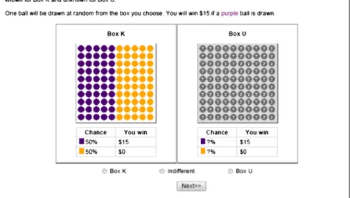
The ALP module posed questions similar to those in a standard Ellsberg experiment with two urns9asking respondents to choose between anambiguousBox U (Unknown) and anunambiguousBox K (Known), following the elicitation method of Dimmock et al. (2015b). Both boxes contained 100 balls, which could be purple or orange, as shown in Fig.1. The respondent was told that one ball would be randomly drawn from the box he selected and he would win $15 if that ball was purple. For Box K, the respondent could see its content on the screen: 50 purple balls and 50 orange balls. The content of Box U is not shown, creating ambiguity. A preference for Box K over Box U indicates ambiguity aversion.
Apart from choosing Box K and Box U, respondents could also choose BIndifferent^. A choice of Indifferent implies ambiguity neutrality, with the subject treating Box U as if the probability of winning were 50% as in Box K. In cases where the subject did not select Indifferent in the first round, he was presented
7
For more information about how the ALP recruits respondents see the American Life Panel website at
https://mmicdata.rand.org/alp/. One advantage of the ALP is that respondents who lack Internet access are provided with either a laptop and Internet access, or a so-called WebTV that allows them to use their television to participate in the panel.
8
Dimmock et al. (2015a) describe the fielding of the ALP module in more detail.
9
additional question rounds similar to the one in Fig.1. For example, if the respon-dent selected Box K in Fig.1, the known probability of winning was then reduced to 25% in the second round; if he chose Box U, the known probability of winning was increased to 75%. This process was repeated for up to four rounds, to closely approximate the respondent’s indifference point. The known probability that makes the respondent indifferent when comparing Box K and Box U is defined as the
matching probability.10
Let m50 denote the matching probability for Question 1. We can then measure ambiguity aversion as follows: AA50=50 %−m50. Positive values of AA50 imply ambiguity aversion, negative values indicate ambiguity-seeking behavior, and a value of zero shows ambiguity neutrality. For example, consider a respondent whose matching probability is 30% (m50=0.3), implying he is indifferent between Box K and Box U when Box K offers a known probability of winning of exactly 30%. He only prefers the ambiguous Box U when Box K offers a probability of winning less than 30%. This behavior is consistent with ambiguity aversion.
Fig. 1 First ambiguity question: winning for one of two ball colors.Notes:This figure shows the first round in the ambiguity question sequence with two ball colors. The respondent can win a prize of $15 if a purple ball is drawn from the box of his preference. Box K contains 50 purple and 50 orange balls, offering 50% initial known probability of winning. Box U also contains purple and orange balls, but with the proportions unknown. If the respondent selectsBBox K^orBBox U^, a second question round follows, similar to the one shown above. If the response isBBox K^, in the second round the probability of winning for Box K is decreased (fewer purple balls). Vice versa, when the respondent selectsBBox U^, in the second round Box K offers a higher probability of winning (more purple balls). Selecting theBIndifferent^button takes the respondent to the next ambiguity sequence, shown in Fig.2
10
This approach is similar to that of Kahn and Sarin (1988), Baillon et al. (2012), Baillon and Bleichrodt (2015), and Dimmock et al. (2015b).
We note that, in theory, a preference for Box K over Box U in the first question round shown in Fig.1can be reconciled with subjective expected utility if a subject assigned a low subjective probability to drawing a purple ball from Box U (e.g., perhaps due to distrust of the surveyor). Nevertheless, the Ellsberg (1961) paradox then arises, because people are also indifferent between betting on drawing anorange
ball from Box U versus betting on drawing apurpleball from Box U, which implies the subjective probabilities sum to less than 100%. Both lab experiments and field studies confirm that people are indeed indifferent about the winning color for Box U.11
To keep the questions as simple as possible for a survey of the general population, we did not include an option to change the winning color. The ALP survey is administered by the RAND Corporation, which our respondents trust to provide the payoffs as they have participated in other previous surveys with this organization. To test the assumption of no color preferences, we fielded an additional survey in which 250 respondents had the option to select their winning color, and a control group of 250 respondents did not. We find no significant differences in ambiguity attitudes between the two groups.12
The elicitation method presents subjects with a series of binary choices converging to the matching probability, instead of directly asking for the matching probabilities, as prior studies have shown that this produces more reliable measures of preferences (see, e.g., Bostic et al. 1990). Because eliciting ambiguity preferences is known to be sensitive to measurement error and within-person inconsistencies (see, e.g., Binmore et al.2012; Stahl2014), the module included two consistency check questions. These check questions are similar to Fig.1, but with the known probabilities of winning for Box K changed tom50+10% andm50–10%, respectively, wherem50is the subject’s matching probability. A preference for Box U in the first check question is inconsistent with earlier choices, as is a preference for Box K in the second check question.
2.2 Eliciting ambiguity attitudes for low and high likelihood events
Although exact probabilities for ambiguous events are unknown, it is often still possible to assess whether an event is unlikely (e.g., the U.S. inflation rate exceeding 10% next year) or highly likely (e.g., the U.S. having positive GDP growth next year). Prior studies reveal that most people are ambiguity seeking for low likelihood ambig-uous events, while ambiguity aversion is common for high likelihood events. Such preferences can be interpreted as a tendency to regard all ambiguous events as if they are 50–50%, or showing too little sensitivity to the likelihood of events (Abdellaoui et al. 2011). This effect is called ambiguity-generated likelihood insensitivity, or a-insensitivity.
11
See, for example, Abdellaoui et al. (2011) and Dimmock et al. (2015b). The latter study finds that fewer than two percent of respondents changed the winning color.
12
In August 2013, we fielded an additional survey (N=500) identical to the original except one: it offered some respondents a choice for the winning ball color. Specifically, a randomly selected half of the sample was allowed to select the winning color (purple or orange), while the other half could not. Fewer than one percent of the respondents in the group allowed to change the color did so, and the mean matching probabilities of the
‘color choice’and‘no color choice’subgroups were not significantly different. Results are available upon request.
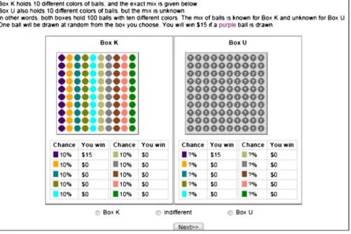
To measure a-insensitivity the survey module included two additional sets of questions with boxes containing balls of 10 different colors. For instance, Fig.2shows the second ambiguity question, where the respondent won $15 if a purple ball was drawn. Here Box K offers a known probability of winning of 10%, while for Box U the probability is unknown. The third question is similar, but with the outcomes reversed: now, the subject won $15 if any of the nine colorsother thanpurple was drawn, and thus for Box K the initial probability of winning is 90%. We definem10andm90as the matching probabilities for these two questions, which are calculated after a maximum of four rounds of bi-section.
The ambiguity aversion measures for these two questions are defined as: AA10= 10%–m10, andAA90=90%–m90. Subjects who selected Indifferent in the first round are ambiguity neutral, withAA10=0 andAA90=0. A-insensitivity predicts that subjects are ambiguity seeking for low likelihood ambiguous events (AA10< 0), and ambiguity averse for high likelihood events (AA90> 0). Hence, we describe a respondent as a-insensitive if AA90–AA10> 0, a-neutral if AA90–AA10= 0, and a-oversensitive if AA90–AA10< 0.
Fig. 2 Second ambiguity question: winning for one of ten ball colors.Notes:This figure shows the first round in the second ambiguity question sequence, with 10 ball colors. Here the respondent wins if a purple ball, 1 out of 10 colors, is drawn from the box of his preference. Box K contains 10 balls of each color and offers a 10% probability of winning. Box U also contains balls with 10 different colors, but with the proportions unknown. If the respondent selectsBBox K^orBBox U^, a second question round follows, similar to the one shown above. If the response isBBox K^, in the second round the probability of winning for Box K is decreased (fewer purple balls). Vice versa, when the respondent selectsBBox U^, in the second round Box K offers a higher probability of winning (more purple balls). Selecting theBIndifferent^button takes the respondent to the next ambiguity sequence: wining for nine out of ten ball colors
2.3 Eliciting ambiguity attitudes for losses
The last module question assesses ambiguity aversion when the outcomes involve losses. Once again, subjects had a choice between Box K with 50 purple and 50 orange balls, and Box U with purple and orange balls in unknown proportions. The subject would now, hypothet-ically,lose$15 if a purple ball were drawn from the chosen box. For losses, we usem−50to denote the matching probability, and the ambiguity aversion measure is:AA−50=m−50–50%.
Subjects are ambiguity averse in the loss domain ifAA−50>0, implying they are prepared to accept a relatively high known probability of losses to avoid Box U.
When choices in the loss domain are incentivized, the standard approach is to give all respondents an initial endowment (e.g., $15) and then subtract subsequent losses. A draw-back of this approach is that it can introduce a house money effect. Additionally, rational respondents who evaluate outcomes in terms of terminal wealth will not experience any losses but only gains and zero outcomes. For these reasons, we do not implement real losses in our module. Etchart-Vincent and l’Haridon (2011) have extensively tested the effect of real incentives in controlled experiments for both gains and losses, and they found that real and hypothetical choices differ significantly only in the gain domain, but not in the loss domain.13
2.4 Summary of ambiguity attitudes in the U.S. population
Table 1 summarizes ambiguity attitudes for our representative sample of the U.S. population. Panel A reports the proportions of people whose responses indicate ambi-guity aversion, seeking, or neutrality. For events of moderate and high likelihood involving gains, most people’s choices were consistent with ambiguity aversion. For example, for the first ambiguity question with two ball colors over half of the respon-dents (52%) make ambiguity-averse choices, only 10% were ambiguity neutral, and 38% were ambiguity seeking. Hence, ambiguity attitudes are heterogeneous, and ambiguity aversion is far from universal. This finding is consistent with other field data studies,14and experimental studies summarized in Trautmann and van de Kuilen (2015). For the high likelihood event (winning if any of nine of the 10 colors is selected), 58% of our respondents were ambiguity averse and only 30% sought ambiguity. By contrast, for the low likelihood event (winning if one of the 10 colors is selected), 60% of respondents were ambiguity seeking and only 19% were ambiguity averse. This provides strong evidence of a-insensitivity, the tendency to treat all ambiguous events as equally probable. Indeed, Panel B of Table1shows that 81% of the respondents were a-insensitive (AA90>AA10).
Panel C provides summary statistics for the matching probabilities and the ambigu-ity aversion measures. For example, the median respondent was indifferent between a known probability of 47% winning for Box K versus betting on one of two colors in Box U, indicating a low degree of ambiguity aversion (median AA50=0.50–0.47= 0.03). For the high likelihood event, the median attitude indicates relatively strong
13Similarly, Baillon and Bleichrodt (2015) find no significant differences between ambiguity attitudes in the
loss domain measured with real incentives and with hypothetical losses.
14Butler et al. (2014) report that 52% of 1686 Italian bank customers are ambiguity averse (without real
incentives), while in Akay et al. (2012) 57% of 92 Ethiopian farmers are ambiguity averse. In a sample of 666 subjects from the Dutch population, Dimmock et al. (2015b) find that 68% were ambiguity averse, 10% neutral, and 22% seeking, suggesting that ambiguity aversion is more common among the Dutch.
ambiguity aversion (median AA90=0.13), while for the low likelihood event the median implies ambiguity-seeking behavior (median AA10=−0.075).
Turning to the loss domain, Panel A reveals that ambiguity seeking is the most common response (40%), followed by aversion (33%), and neutrality (27%). The
Table 1 Descriptive statistics for ambiguity attitudes
Panel A. Ambiguity attitudes (Proportion of respondents for each question)
Ambiguity Question Gains 10% Gains 50% Gains 90% Losses 50%
Ambiguity averse 18.5 52.4 57.7 33.6
Ambiguity neutral 21.5 9.9 12.8 26.9
Ambiguity seeking 60.0 37.7 29.5 39.6
Panel B. A-Insensitivity Percent of respondents A-Insensitive (AA90–AA10>0) 80.5
Neutral (AA90–AA10=0) 7.5
A-Oversensitive (AA90–AA10<0) 12.0
Panel C: Summary statistics of matching probabilities and ambiguity aversion
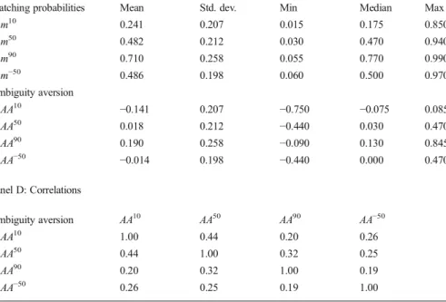
Matching probabilities Mean Std. dev. Min Median Max
m10 0.241 0.207 0.015 0.175 0.850 m50 0.482 0.212 0.030 0.470 0.940 m90 0.710 0.258 0.055 0.770 0.990 m−50 0.486 0.198 0.060 0.500 0.970 Ambiguity aversion AA10 −0.141 0.207 −0.750 −0.075 0.085 AA50 0.018 0.212 −0.440 0.030 0.470 AA90 0.190 0.258 −0.090 0.130 0.845 AA−50 −0.014 0.198 −0.440 0.000 0.470 Panel D: Correlations Ambiguity aversion AA10 AA50 AA90 AA−50 AA10 1.00 0.44 0.20 0.26 AA50 0.44 1.00 0.32 0.25 AA90 0.20 0.32 1.00 0.19 AA−50 0.26 0.25 0.19 1.00
Notes: This table shows ambiguity attitudes in the U.S. population measured in our ALP module (see text). We posed three ambiguity gains questions with ambiguity-neutral probabilities of 10%, 50%, and 90% for Box U, where subjects could win $15, and one 50% question with hypothetical losses of -$15. Panel A displays the proportion of respondents who are ambiguity averse, ambiguity seeking, or ambiguity neutral, based on their choice between Box K and Box U in the first round of each ambiguity question. Panel B summarizes a-insensitivity. Panel C shows summary statistics for the matching probabilities and ambiguity aversion measures for each question separately. Panel D presents correlations of the four ambiguity aversion measures. The sample consists of 2991 people who answered all ambiguity questions and spent at least two minutes of time. All results use ALP survey weights
average degree of ambiguity aversion for losses is close to zero, due to the strong heterogeneity in attitudes. To examine reference dependence, we test the null hypoth-esis that mean AA50=meanAA−50. A paired samples t-test strongly rejects the null hypothesis of ‘no reference dependence’ (p-value<0.01); accordingly, ambiguity aversion differs for gains and for losses in the general population, consistent with the experimental results of Cohen et al. (1987), Abdellaoui et al. (2005), and Baillon and Bleichrodt (2015). We next test for reflection, or mean AA50=−meanAA−50, which implies that ambiguity aversion for gains is reflected into ambiguity-seeking behavior for losses. In this case the null hypothesis ‘reflection’ cannot be rejected (p-value=
0.411).15Using experimental data, Vieider et al. (2012) and Kothiyal et al. (2014) also found reflection at the aggregate and individual level for decisions under ambiguity.
Finally, Panel D of Table1reports positive and significant correlations between all four question-specific measures of ambiguity attitudes. Hence, although ambiguity aversion does differ across likelihoods and for gains versus losses, the estimates are all positively related. This is consistent with a common underlying factor driving ambiguity aversion across domains.
In results not reported in detail here (see OnlineAppendix A), we also examine respondent consistency with the two check questions mentioned above. We find that 41% of the respondents answer both check questions correctly, while 17% give both consistent and indifferent answers. The remaining 42% of our respondents contradict an earlier choice once (39%) or twice (3%). The consistency rates are low, but similar to earlier findings in the Netherlands (Dimmock et al.2015b) and in experimental settings (e.g., Trautmann and van de Kuilen 2015). As an important robustness check, all estimates in Section 4 are repeated in the full sample as well as the subset of respondents who passed both consistency checks (see Section4.3).
3 Multiple prior models for decision-making under ambiguity
We next specify a tractable version of theα-MaxMin model, which can be estimated using the matching probabilities observed in the survey data. The model has two parameters:α, which measures ambiguity aversion; andδ, which measures the degree of perceived ambiguity relative to a reference distribution in which the decision-maker has limited confidence.
3.1 Theα-MaxMin model
We model uncertainty using astate space Sconsisting of a finite number of future states of the world (s1,s2,…,sn). One statesϵSis true and the other states are not, but which
state is true is uncertain. Subsets of the state space are calledevents. For example, event
E={s1,s3,s6} is true if the state iss1,s3, ors6. The set containing all possible events is
denoted by Θ. A probability measure P is a function P:Θ→ℝ that assigns real numbers between 0 and 1 to events, with the following properties:P(Ø)=0,P(S)=1,
P(E)≤P(F) for all eventsE,F∈ΘwithE⊆F, andP(E∪F)=P(E)+P(F)−P(E∩F). LetΓ
15
A signed rank test for the median gives similar results:p-value<0.01 for no reference dependence (median AA50= median AA−50);p-value=0.13 for reflection (median AA50=−median AA−50).
denotes the set of all possible probability measures. A prospectxis a function assigning outcomes to events,x:Θ→ℝ, giving monetary amount x(E) if event E occurs. For example, in our experiment with ambiguous Box U, there are two states,s1=a purple ball is drawn, ands2=an orange ball is drawn, with respective outcomes x(s1)=$15 and x(s2)=$0. Finally, we assume that the decision-maker has an increasing utility function
U:ℝ→ℝover outcomes.
Ambiguity occurs when the decision-maker does not know the exact probabilities of all eventsEinΘ. Multiple prior models assume that the decision-maker considers a convex setCof possible probability measuresPϵC. In the multiple prior model of Gilboa and Schmeidler (1989), the decision-maker uses the worst distribution inCto evaluate prospects, as follows:
M axM in xð Þ:minP∈CEP½U xð Þ ¼minP∈C
∫
s∈SU x sð ð ÞÞdP sð Þ ð1Þ whereEP[U(x)] denotes the expected utility of prospectxunder probability measureP,andxis shorthand notation forx(s).
When choosing between prospectsxandy, the decision-maker strictly prefersxover
yif and only if minP∈CEP[U(x)]>minP∈CEP[U(y)]. Hence, the decision-maker acts as if
he maximizes the minimum expected utility value, giving rise to the name MaxMin. The MaxMin model implies that the decision-maker is ambiguity averse or pessimistic, as he evaluates prospects based on the prior probability distribution giving the lowest expected utility.
Ambiguity-seeking behavior is consistent with Equation (1) if we replace the minimum over P by the maximum, which is called the MaxMax model. The α-MaxMin model combines these two extremes, with weightαϵ[0,1]:
αM axM in xð Þ:αminP∈CEP½U xð Þ þð1−αÞmaxP∈CEP½U xð Þ ð2Þ Thus the α-MaxMin model can accommodate both ambiguity-averse and ambiguity-seeking behavior.16Furthermore, the set of prior distributionsCnow reflects perceived ambiguity, whileα is a measure of aversion to this ambiguity. Maximum ambiguity aversion occurs at the value α=1 (MaxMin), and maximum ambiguity seeking atα=0 (MaxMax).
3.2 The multiple prior set
A complication in empirically implementing theα-MaxMin model is the specification and estimation of the set of priorsC. In a real-world setting such as investing, it can be difficult for decision-makers to indicate exactly which prior probability distributions they consider plausible. Previous literature on ambiguity often adopts a specification forCtermedε-contamination(e.g., Epstein and Wang1994). The approach assumes that the decision-maker has a reference probability distribution,π, which is an assess-ment of the probability of events based on his subjective beliefs. The decision-maker is aware, however, that he does not know the true probabilities, so he considers all
16
Ghirardato et al. (2004) and Eichberger et al. (2011) provide a behavioral (i.e., axiomatic) foundation for the
distributions in the larger setCε={Q∈Γ:Q=(1−ε)π+εP,forP∈D}, withε ϵ[0,1] and
Dis a given set of contaminating probability measures. Henceπis contaminated with distributions from the setD, with the parameterεdetermining the perceived level of ambiguity. In empirical applications, though, researchers still must specify or estimate the set of contaminating probability distributionsD.
In our specification of perceived ambiguity, we adhere to the concept of a reference distributionπ. Following Chateauneuf et al. (2007), we assume the decision-maker has a degree of confidence (1−δ) in π, with δ ϵ [0,1]. He then considers the set Cδof probability measuresPassigningat leastprobability (1-δ)π(E) to all eventsE:
Cδ¼fP∈Γ :P Eð Þ≥ð1−δÞπð ÞE ;for allE∈Θg;withδ∈½0;1 ð3Þ At first glance,Cδappears to provide only lower bounds on probabilities. But we note that inequality (3) also holds for each eventE’s complement, defined asEc=S\E.17Thus
P(Ec)≥(1−δ)π(Ec). UsingP(Ec)=1−P(E), we get 1−P(E)≥(1−δ)(1−π(E)), which gives the following upper bound:P(E)≤1−(1−δ)(1−π(E))=(1−δ)π(E)+δ. Accordingly, the set of priorsCδimposes the following bounds on the probability measuresP∈Cδ:
0≤ð1−δÞπð ÞE ≤P Eð Þ≤ð1−δÞπð Þ þE δ≤1;for allE∈Θ ð4Þ The prior setCδallows the probabilityP(E) to vary in an interval of lengthδaround the reference probabilityπ(E).18We note that the reference probabilityπ(E) does not necessarily lie in the middle of the interval: this is only case forπð Þ¼E 0:5 orδ=0. For
πð ÞE <0:5, the interval will be longer aboveπ(E) than belowπ(E), and vice versa when
πð ÞE >0:5. This feature is important for explaining ambiguity-seeking behavior for low
likelihood events but ambiguity aversion elsewhere, as we will explain later.
The prior set Cδ for α-MaxMin, originally introduced by Chateauneuf et al. (2007), is useful in empirical applications for several reasons. First, the per-ceived level of ambiguity is captured by δ and the standard subjective expected utility framework is a special case when δ= 0. Second, instead of eliciting the decision-maker’s entire set of possible priors C (or the set D), we simply specify one reference distribution π and estimate the confidence level (1-δ). In applications with Ellsberg urns, the values for π follow naturally from symmetry conditions. In stock market applications, a good candidate for π would be the estimated return distribution based on historical data.19 Third, Chateauneuf et al. (2007, Remark 3.2) show that the α-MaxMin model with prior set Cδ is equivalent to their Choquet expected utility model with a neo-additive capacity, and they provide an axiomatic foundation for the latter.20In this way, the
17
Eccontains all statessexcept those contained in eventE:E∪Ec=SandE∩Ec=∅.
18
Note thatP(E)=0 forE∈N, whereNdenotes a set of all null eventsE∈Nwithπ(E)=0.
19
Given sufficient experimental time one could elicit a subjective measureπfor uncertain events from revealed preferences at the individual level as in Abdellaoui et al. (2011).
20The measures of ambiguity aversion and a-insensitivity introduced by Abdellaoui et al. (2011), namedIndex bandIndex a, also derive from a neo-additive capacity and can therefore be linked toαandδ. That is, for their a-insensitivity measure:Index a=δ. For their ambiguity aversion measure:Index b=(2α−1)δ. Hence, Indexb
preference ordering implied by the model satisfies important properties such as complete-ness, reflexivity, and transitivity.
3.3 Theα-MaxMin model with prior setCδapplied to our experiment
For our first survey question, Box U contained 100 balls, each having one of two possible colors, purple or orange, with the proportions unknown. One ball was drawn randomly from Box U and the respondent won $15 if the ball was purple, and nothing otherwise. ForS={s1,s2}, state s1denotes a purple ball was drawn, and similarlys2 denotes an orange ball was drawn. The outcomes arex(s1)=$15 andx(s2)=0, evaluated with utility function U. The utility function can be rescaled such that U(0)=0 and
U(15)>0. The α-MaxMin model with prior distribution set Cδ then evaluates the prospectxas follows:
α minp∈½ð1−δÞπ;ð1−δÞπþδpUð Þ þ15 ð1−αÞmaxp∈½ð1−δÞπ;ð1−δÞπþδpUð Þ15 ¼αð1−δÞπUð Þ þ15 ð1−αÞðð1−δÞπþδÞUð Þ15
¼ðð1−δÞπþð1−αÞδÞUð Þ15
ð5Þ
whereπ=π(s1) is the reference probability of drawing a purple ball from Box U. Box K offers a known probabilitypof winning the $15 prize and it is evaluated with expected utility (δ=0), giving: E[U(x)]=pU(15). The matching probability m is the known probabilitypthat makes the respondent indifferent when comparing Box K and Box U. Respondents are indifferent between the two when ((1−δ)π+(1−α)δ)U(15)=
pU(15), so the matching probabilitymis:
m¼ð1−δÞπþð1−αÞδ ð6Þ
We note that the utility function cancels out in the comparison, so we need not estimate utility (or risk aversion) in order to measure people’s ambiguity attitudes: this is a major advantage of the elicitation method.
Similar to what is shown in Section3.1, once we know the matching probability, we can define an index of ambiguity aversion as:AA=π−m=(α−(1−π))δ. It follows that in the special case of no perceived ambiguity,δ=0, the matching probability isπand respondents are ambiguity neutral (AA=0). For respondents who perceive some ambi-guity about the exact probability of winning for Box U,δ>0, the ambiguity attitudes are:
AA>0: if α>1−π and δ>0;
AA¼0: if α¼1−π and δ>0;
AA<0: if α<1−π and δ>0:
ð7Þ We takeπ¼0:5 as the relevant reference probability for drawing a purple ball from Box U, assuming indifference between having purple or orange as the winning color. The result above implies decision-makers perceiving some degree of ambiguity about the number of purple balls in Box U (δ>0) will be ambiguity averse in our first ambiguity question (AA>0) if α>0:5, ambiguity seeking (AA<0) if α<0:5, and ambiguity neutral (AA=0) ifα¼0:5.
We repeat this analysis for our second ambiguity question where Box U contained 100 balls with 10 different colors, and the prize of $15 was won if one particular color was drawn. It is easy to show that Equations (5), (6), and (7) still hold. The only difference is that the reference probability for winning for one out of 10 possible colors isπ=1/10. Equation (7) now predicts ambiguity-averse responses in the first round of the second question ifα>0.9 andδ>0. Hence, only individuals with very high levels of ambiguity aversion would still prefer Box K, and ambiguity-seeking choices are expected to prevail.
The explanation for this effect is that atπ=1/10, the interval of prior probabilities used by the decision-maker is asymmetric around π: [(1-δ)0.1, (1-δ)0.1+δ]. For example, with a confidence level of 80% (δ=0.2), the interval is [0.08, 0.28]. The upper bound of the interval is much further aboveπthan the lower bound is below it. The result is that the‘max’inα-MaxMin will influence the result more than the‘min’, and theα-MaxMin value of Box U will exceedπU(15). The decision-maker will prefer Box U and display ambiguity seeking behavior, unless his ambiguity aversion α is sufficiently high (precisely, only ifα>0.9).
The intuition for the asymmetric prior aroundπ=1/10 follows from the fact that the prospect offers positive skewness: on the positive side the number of winning balls in Box U can range from 10 to 100, while on the negative side it can only range from zero to 10. Accordingly, the interval of prior probabilities reflects that perceived ambiguity should be higher on the upside (p>0.1) than on the downside (p<0.1). Andersen et al. (2012, Fig. 6) explicitly estimated the distribution of prior probabilities for an ambig-uous event withπ=1/10 in a sample of students and found that it was indeed highly positively skewed.
Similarly, Equations (5), (6), and (7) also apply to the third ambiguity question, where the respondent wins if any of the nine of the 10 ball colors is chosen, with reference probabilityπ=9/10. We can deduce that ambiguity-averse responses will occur in the third ambiguity question ifα>0.1 andδ>0. The interval of prior proba-bilities is again asymmetric. For example, with a confidence level of 80% (δ=0.2), the interval is [0.72, 0.92]. In this case, it is natural for the decision-maker to perceive more ambiguity on the downside than on the upside, as the number of winning balls in U could be far less than the reference number of 90 balls. Experimental results in Andersen et al. (2012, Fig. 6) support this: the estimated prior distribution for an ambiguous event withπ=8/10 is strongly negatively skewed.
The fourth question involved a hypothetical loss of $15 and two colors of balls. Here the matching probability ismL=(1-δ)π+αδ, as detailed in Online Appendix B. For losses, a subject was ambiguity averse if he was willing to accept a relatively high known probability of loss to avoid Box U, that ismL>π, corresponding toα>0.5 (see OnlineAppendix B).
3.4 Alternative multiple prior sets for theα-MaxMin model
We now derive the matching probability for two alternative prior sets, which we will also estimate and evaluate against our proposed model. First, in the special case of zero confidence (δ=1), the prior interval is [0, 1], and the decision-maker then considers all possible probabilities. The matching probability in this case is:m=(1-α). We note that
m is independent of π, implying that the matching probability is the same for all ambiguity questions.
Second, we introduce an alternative prior probability setCsym, which is symmetric
around the reference probabilityπ:
Csym¼ p∈ π− 1 2d;πþ 1 2d
;withd≥0 andd≤min 2f π;2 1ð −πÞg ð8Þ wherepis a prior probability of winning, anddis the length of the prior probability interval. Using this prior interval, a prospect paying $15 if a purple ball is drawn from Box U is evaluated as:
αminp∈½π−0:5d;πþ0:5dpUð Þ þ15 ð1−αÞmaxp∈½π−0:5d;πþ0:5dpUð Þ15
¼α πð −0:5dÞUð Þ þ15 ð1−αÞðπþ0:5dÞUð Þ ¼15 ðπþð0:5−αÞdÞUð Þ15 ð9Þ Accordingly, the matching probability ism=π+(0.5–α)d, andAA=π-m=(α-0.5)d. The decision-maker is ambiguity neutral (AA=0) ifd=0 orα=1/2, ambiguity averse (AA>0) ifα>1/2 andd>0, and ambiguity seeking (AA<0) ifα<1/2 andd>0. We note that the ambiguity attitude (AA) is independent of the reference probability, and thus this model cannot explain a-insensitivity. Further, the model implies that in a regression of m on π the slope coefficient of π is equal to 1, a condition that we can test empirically.
4 Estimating the
α-MaxMin model 4.1 Econometric modelFor our econometric model, we adopt the following notation: for each respondent (i=1,2,...,I) and for each of the three ambiguity elicitation questions in the gains domain (k=1, 2, 3), we measure a matching probabilitymik.21Further, letπikdenote the reference
probability of winning for Box U in questionk. We assume that all respondents are neutral about the winning color, so that subscript i can be dropped and πk has the
following fixed values:π1=0.5,π2=0.1 andπ3=0.9. To capture the general tendency of ambiguity attitudes in the population, in our model we initially assume that there is only one representative decision-maker, as is common in the literature on estimating prefer-ence models. Hprefer-ence, the parameters for ambiguity aversionαand the perceived level of ambiguityδare constant, not depending oni. Equation (6) then implies that the matching probabilitymikin theα-MaxMin model is equal to:mik=(1–α)δ+(1–δ)πk, fork=1, 2, 3.
Empirically, we estimate this equation as follows:
mik ¼cþsπkþεik; fori¼1;2…;I and k¼1; 2; 3 ð10Þ wherecandsare coefficients, andεikis an identically and independently distributed
error term.
21
Model (10) can be estimated with pooled ordinary least squares (OLS), with k
observations for each respondent. The parameters of theα-MaxMin model are identi-fied asδ=1–sandα=1–c/δ. Standard errors forδandα are computed with the delta method. We can now test and compare the fit of different versions of theα-MaxMin model using the following restrictions:
EU expected utilityð Þ:δ¼0 andc¼0 ð11aÞ
αMaxMinCsym:δ¼0 andc≠0 ð11bÞ
MaxMin½0;1:δ¼1 andα¼1 ð11cÞ
MaxMax½0;1:δ¼1 andα¼0 ð11dÞ
αMaxMin½0;1:δ¼1 and 0<α<1 ð11eÞ
MaxMinCδ:0<δ<1 andα¼1 ð11fÞ
MaxMaxCδ:0<δ<1 andα¼0 ð11gÞ
αMaxMinCδ:0<δ<1 and 0< α<1 ð11hÞ HereCsymis a symmetric prior probability interval (of unknown length d), while
[0,1] denotes the prior interval where the decision-maker considers all possible prob-abilities, and Cδthe asymmetric prior probability set where the decision-maker has confidence (1–δ) in the reference probabilityπ. Tests of restrictions (11a–h) allow us to see which specification ofα-MaxMin best describes the general pattern of ambiguity attitudes in the U.S. population.
To loosen the restrictive assumption of one representative decision-maker and to take into account heterogeneity in ambiguity preferences (see, e.g., Stahl2014), we include a random effect in the model:mik=c+sπk+εik+ui, whereuiis a random effect
that is independent of the error term (εik) and uncorrelated between individuals, with E[ui2]=σu2. The random effect captures unobserved heterogeneity in the ambiguity
aversion parameter αi across individuals i, with αi=1−(c+ui)/δ. Finally, we use
clustered standard errors to correct for heteroskedasticity between individuals, and correlation of the error terms within.
4.2 Main results
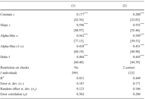
Table2displays our estimates of the constantcand the slope coefficients. Additionally, the table shows estimates for the α-MaxMin model parameters α, (1–α), and δ, to facilitate interpretation and testing of hypotheses. Column (1) reports estimates for our baseline sample consisting of 2991 respondents who answered all ambiguity questions and who spent at least two minutes answering the ambiguity questions.22The depen-dent variables are the matching probabilities,mikfor the first three ambiguity questions
(k=1, 2, 3), involving only gains and implemented with real incentives. We discuss the results for losses in a later section. The estimates shown in Table2are for a random effects model specification; estimates for the model without random effects in (10) are similar and therefore not reported.23
Our baseline results show that, overall, the U.S. population is ambiguity averse. Column (1) of Table2reportsα=0.56, combined with 60% confidence in the reference probability (δ=0.40).24The extent of ambiguity aversion is modest, with only a slight overweighting of the worst outcome (α>1/2). Nevertheless, it is statistically significant as we can rejectα≤1/2 (t=8.47 andp-value<0.01). Together, these estimates (α=0.56,
δ=0.40) imply ambiguity-seeking behavior for the low likelihood ambiguous event of winning if one of 10 possible colors is chosen. Here, our model predicts a matching probability of 0.24. The estimates also imply relatively strong ambiguity-averse behav-ior for the high likelihood ambiguous event of winning if any of nine of 10 possible colors is selected; the model predicts a matching probability of 0.71. Hence, theα -MaxMin model with prior setCδdescribes the typical pattern of ambiguity attitudes in the population well, including a-insensitivity.
We use the model estimates in Column (1) to test the alternative multiple prior models in hypotheses (11a-h) in subsequent steps. First, the data do not support subjective expected utility with reference probability measure π (11a): a joint test rejects the restrictionsc=0 andδ=0. Second, the use of a pessimistic prior probability set [0,1] for theα-MaxMin model is not supported: hypotheses (11c-e) impose the restrictionδ=1, which is rejected.25Third, the symmetric prior probability setCsymfor
theα-MaxMin model is also inconsistent with the data: the restrictionδ=0 in (11b) is rejected. Among the models based on the prior set Cδ, the pessimistic MaxMin-Cδ
22
Out of the 3258 original respondents, 3 did not answer any questions, 85 did not complete all of our ambiguity questions, and 179 spent less than two minutes on answering the ambiguity questions. After excluding these 267 respondents, we have a final sample of 2991 respondents.
23Pooled OLS estimates are consistent in the presence of random effects, but the standard errors may be
inefficient. As we use clustered (robust) standard errors, the results of pooled OLS are similar to a random effects model.
24
Our estimate ofαis similar to values ofα=0.515 reported in Ahn et al. (2014) for a small sample of students andα=0.556 in Potamites and Zhang (2012) for Chinese investors. Baillon et al. (2015) estimateα= 0.61 andδ=0.51 in a sample of 64 students, with the source of ambiguity being the returns of an unknown stock.
25
We test the single restrictionδ=1, implied by all three models with [0,1] as the prior set. Joint tests ofδ=1,
model (11f) and the optimistic MaxMax-Cδ(11g) are also both rejected, as they imply
α=1 andα=0. Only theα-MaxMin model with prior setCδ(0<δ<1) and 0<α<1) is consistent with the pattern of ambiguity attitudes in the U.S. population.
In sum, we find support for ambiguity preferences where not all the weight is put on the worst case (α=1) nor on the best case (α=0), and the prior probability set reflecting ambiguity perceptions is asymmetric for allπ≠0.5.
4.3 Robustness checks
As a robustness check, we next exclude respondents who gave incorrect answers to the two check questions: Column (2) limits the sample to respondents who answered both check questions correctly. Interestingly, the coefficient estimates change hardly at all, and our conclusions remain the same. For example, ambiguity aversion and confidence in the reference probability are both slightly lower among respondents who answered both check questions correctly (α=0.55,δ=0.45), but the difference is small compared to the full sample results.
Statistical tests (available on request) confirm that a random effects model fits our data better than pooled OLS or fixed effects models. The row labeledBError correlation
Table 2 Alpha-MaxMin model estimates
(1) (2) Constantc 0.177*** 0.200*** [42.56] [32.03] Slopes 0.596*** 0.555*** [88.97] [55.46] Alpha-Minα 0.562*** 0.549*** [77.13] [59.53] Alpha-Max (1-α) 0.438*** 0.451*** [60.19] [48.90] Deltaδ 0.404*** 0.445*** [60.40] [44.39]
Restriction on checks No 2 correct
Iindividuals 2991 1232
R2 0.431 0.449
Error st. dev. (σε) 0.187 0.171
Random effect st. dev. (σu) 0.123 0.106
Error correlation (ρ) 0.302 0.280
Notes:The table shows estimation results for theα-MaxMin model, derived from matching probabilitiesmik
for the three ambiguity gain questions (k=1, 2, 3). We estimate Equation (10) using a random effects model, which gives estimates of the slope coefficientsand constantc. Estimates of ambiguity aversion parameterα and perceived ambiguityδare then derived fromcands, with standard errors based on the delta method. Column (1): full sample results. The full sample consists of respondents who answered all ambiguity questions and spent at least two minutes of time. Column (2): same model, but further limited to 1232 respondents who answered both check questions correctly. Standard errors are shown in brackets (robust, clustered by individual). Statistical significance:*p<0.1,**p<0.05,***p<0.01
(ρ)^ in Table2 shows the estimated within-individual correlation of the overall error term (εik+ui, including the random effectui):ρ=0.30. The significance ofρindicates
unobserved heterogeneity in ambiguity aversion at the individual level; the variance of the errors (σε2) drops by 30% after accounting for this unobserved heterogeneity.
In additional results (available on request), we estimate a model with a random effect added to the slope coefficient (s+vi), to capture unobserved heterogeneity in ambiguity
perceptions (δ). The main coefficient estimates are unchanged (α=0.56, δ=0.40), as random effects only alter the covariance matrix of the errors. But, the variance of the errors (σε2 = 0.1642) drops by another 23% after taking into account unobserved heterogeneity in perceived ambiguity. Further, posterior estimates ofαandδshow a positive correlation between ambiguity aversion and perceived ambiguity, ranging from 0.2 to 0.4. Hence, those who perceive more ambiguity also tend to be more ambiguity averse.
4.4 Ambiguity attitudes for losses
Next we include the matching probability for the ambiguity question involving losses; our aim is to test whether ambiguity aversion differs for gains and losses. Recall that the matching probability for the ambiguity gains questions ismik=(1−α)δ+(1−δ)πk, for k=1, 2, 3. By contrast, the matching probability for the loss question is:mikL=αLδ+(1 −δ)πk, fork=4 (see OnlineAppendix B). We introduce a separate ambiguity aversion
parameter for losses,αL, distinct fromα, the ambiguity aversion parameter for gains.26 The adapted regression model specification below allows us to test whetherα=αL:
mik ¼cþdLLkþsπkþεikþui; fori¼1;2;…;I and k¼1; 2; 3; 4 ð12Þ whereLkis a dummy variable for the loss question (Lk=0 fork=1, 2, 3, andLk=1 for k=4), and dL is the corresponding regression coefficient. The parameters of the α-MaxMin model are identified as follows:δ=1–sandα=1–c/δ, andαL=(c+dL)/δ.
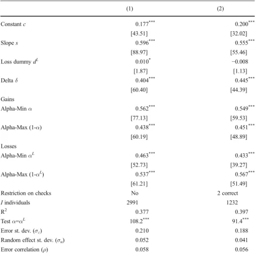
Table3displays estimation results for Equation (12). The row labeledBTestα=αL^ in Table3shows that the data reject the hypothesis that ambiguity aversion for losses and gains are equal. Instead, we find ambiguity aversion for gains (α=0.56) and ambiguity seeking for losses (αL= 0.46).27 We note that the restriction dL= 0 corresponds to the special case ofαL=(1-α), or reflection of ambiguity aversion for gains (α>½) into ambiguity seeking for losses (αL<½). In both columns in Table3, we cannot rejectdL=0 at the five percent significance level.
Reflection implies that the ambiguity attitude for losses is the opposite of that toward gains. Reflection is often found for decisions under risk, and it is part of prospect theory (Tversky and Kahneman1992): a common finding is of risk aversion for gains and risk
26
The equations formikandmikLhave different constant terms, (1–α)δandαLδ, so the model in Equation (11)
is no longer applicable (it would imply the restriction 1–α=αL). Introducing a dummy variable for the loss question permits us to separately estimate and identifyαandαL.
27A drawback of the model in Equation (12) is that the random effectu
ihas opposite effects on ambiguity
aversion for gains and losses, an assumption inconsistent with the positive correlation betweenAA50and AA−50. As a result the estimated correlation of the random effect (ρ) is relatively low in Table3. We have also estimated a model with two separate random effects for the constantcand loss dummydL, but we find no difference in the main results concerningα,αLandδ. Results are available on request.
seeking attitudes for losses. To the best of our knowledge, the results in Table3are the first confirmation of reflection as the typical pattern for decision-making under ambi-guity in the general population. In line with our results, Kothiyal et al. (2014) find evidence of reflection in an experiment with students.
The results in Table 3 are subject to two caveats. First, as explained above, the ambiguity question for losses was implemented without real incentives to avoid house money effects. Second, in Equation (12) we assume that the perceived level of
Table 3 Testing reference dependence: alpha for gains and losses
(1) (2) Constantc 0.177*** 0.200*** [43.51] [32.02] Slopes 0.596*** 0.555*** [88.97] [55.46] Loss dummydL 0.010* −0.008 [1.87] [1.13] Deltaδ 0.404*** 0.445*** [60.40] [44.39] Gains Alpha-Minα 0.562*** 0.549*** [77.13] [59.53] Alpha-Max (1-α) 0.438*** 0.451*** [60.19] [48.89] Losses Alpha-MinαL 0.463*** 0.433*** [52.73] [39.27] Alpha-Max (1-αL) 0.537*** 0.567*** [61.21] [51.49]
Restriction on checks No 2 correct
Iindividuals 2991 1232
R2 0.377 0.397
Testα=αL 108.2*** 91.4***
Error st. dev. (σε) 0.210 0.188
Random effect st. dev. (σu) 0.052 0.041
Error correlation (ρ) 0.058 0.056
Notes:The table shows estimation results for theα-MaxMin model, derived from matching probabilitiesmik
for all four ambiguity questions (k=1, 2, 3, 4), including the question involving losses as outcomes. We estimate Equation (12), which gives estimates of the slope coefficients, constantcand the coefficient for the loss question dummydL. Using these estimates, we then derive values for δ(perceived ambiguity),α (ambiguity aversion for gains), andαL (ambiguity aversion for losses), with standard errors based on the
delta-method. The rowBTestα=αL^displays a chi-square statistic for the null hypothesisα=αL: ambiguity
aversion for gains and losses are equal. Column (1): full sample estimates. Column (2): same model, but limited to 1232 respondents who answered both check questions correctly. Standard errors are shown in brackets (robust, clustered by individual). Statistical significance:*p<0.1,**p<0.05,***p<0.01
ambiguity δis equal for gains and losses.28 This is equivalent to assuming that a-insensitivity is equal for gains and losses, which is supported by experimental evidence in Baillon and Bleichrodt (2015).
4.5 Ambiguity aversion and observed individual characteristics
Little is known about how ambiguity preferences vary with individual characteristics such as gender, age and income. Even less is known regarding individual characteristics andperceptions about ambiguity levels: in this section we are the first to investigate this relation.29Letxihdenote the value of individual control variableh=1, 2,...,H, for person i=1,2,...,I. We estimate the following model:
mik ¼c0þ∑Hh¼1chxihþ s0þ∑Hh¼1shxih
πkþεikþui;
fori¼1;2;…I and k¼1; 2; 3; 4 ð13Þ wherec0is a constant andchis a coefficient for the effect of variableh=1, 2,...,Hon the
constant part of the model. The set of coefficientsshallow the model’s slope coefficient
to depend on the individual attributes, whiles0is the constant part of the slope. The parameters of theα-MaxMin model are identified as:δi=1−(s0+∑Hh=1shxih),andαi=1 −(c0+∑hH=1chxih)/δi.
The individual characteristics available from the ALP include indicators for male; White; Hispanic; married; education (highest degree: high school or college); employ-ment; (ln) family income; (ln) number of children; a financial literacy index; an indicator of trust in others30; risk aversion; and question order. Online Appendix C
provides variable definitions and descriptive statistics. The risk aversion metric is the coefficient of relative risk aversion of a power utility function estimated using questions similar to those in Tanaka et al. (2010).31We randomized the order of the ambiguity and risk questions in the ALP survey, with half of the respondents getting the risk questions first, and the other half the ambiguity questions first. For this reason, we include an indicator equal to one if the subject answered the risk questions first, and zero otherwise.
Table4reports the effects of the individual characteristics on ambiguity aversionα and the perceived level of ambiguityδ, with standard errors derived using the delta
28If we could measure more matching probabilities for ambiguous events involving loss outcomes with other
likelihoods (e.g., similar to the 10 % and 90 % gains questions), we could also estimateδseparately in the loss domain. We leave to future research additional refinements of ambiguity surveys and tests for reference dependence.
29Borghans et al. (2009) find that men are more ambiguity averse than women in a sample of 347 high school
students. In a study of the Dutch population, Dimmock et al. (2015b) estimate the relation between ambiguity attitudes and control variables; there, however, few effects are statistically significant (sample size:N=666). Using our ALP Module, Dimmock et al. (2015a) show in a web appendix that the non-parametric ambiguity aversion measureAA50is higher for men than for women, and positively related to risk aversion.
30This is measured on a reversed scale from 0 to 5, with higher values indicatinglowertrust.
31As in Tanaka et al. (2010), utility is defined over the payoffs of the gambles (not integrated with total
wealth), and the power coefficient is limited to the range from 0 to 1.5. Risk aversion, defined as‘1–power function coefficient’, varies from−0.5 (risk seeking) to +1 (strongest level of risk aversion), and a value of zero implies risk neutrality.
method. Columns (1) and (2) in Table4display marginal effects for ambiguity aversion
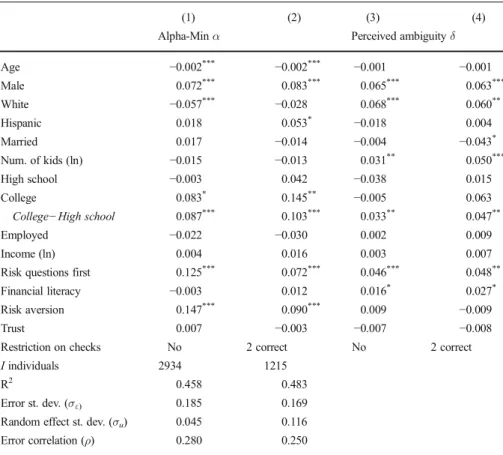
α.32Columns (3) and (4) show the effect of the variables on perceived ambiguityδ. Turning first to ambiguity aversion (α), we find that men are more ambiguity averse than women, consistent with the experimental results in Borghans et al. (2009). Ambiguity aversion is positively related to risk aversion, but the correlation is low and ambiguity aversion is not subsumed by it. Older people tend to be less ambiguity averse, which may capture the effect of life experiences, or a cohort effect. College-educated respondents have higher ambiguity aversion than the less educated. This latter finding is inconsistent with a potential alternative explanation for ambiguity aversion: that it is driven by low cognitive ability. Rather, the positive relation with college education suggests that ambiguity aversion measures preferences rather than cognitive errors.
We also find that ambiguity aversion is higher when the risk aversion questions are presented to respondents prior to the ambiguity questions. The comparative ignorance hypothesis of Fox and Tversky (1995), which states that ambiguity aversion is mag-nified by a comparison to less ambiguous events, predicts such an order effect. In our survey, the comparison is relative to the preceding risk questions involving only known probabilities and no ambiguity. For this reason we randomized the survey order of the risk and ambiguity questions.
Turning to perceived ambiguity (δ), we find that males, whites, and people with more children tend to perceive higher levels of ambiguity. Further, college-educated respondents perceive more ambiguity than high school educated respondents. Receiving the risk aversion questions first also is associated with higher perceptions of ambiguity. Interestingly, age and risk aversion do not influence perceptions about ambiguity levels, but only ambiguity aversion. Vice versa, having (more) children is associated with perceiving more ambiguity, but not with higher ambiguity aversion.
We also investigated how individual attributes are related to ambiguity aversion for losses, and in results not detailed here, we found that the dependent variable is positively related to risk aversion but not significantly associated with the other variables. Thus risk aversion is positively related to both ambiguity aversion for gains and ambiguity aversion for losses, but not related to the perceived level of ambiguity. A potential explanation is that preferences towards risk and ambiguity are related (al-though weakly) as both are preferences, while perceptions about the level of ambiguity are formed independently from risk preferences.
5 Conclusion
This paper develops a method for estimating and testing multiple prior models of ambiguity. Using a nationally representative sample of almost 3000 U.S. respondents, we use matching probabilities to estimate a measure of ambiguity preferences,α, as well as perceptions about the level of ambiguity,δ. Using our simple and tractable method, we estimateαto be equal to 0.56 in the gain domain, consistent with mild ambiguity aversion (α> ½). We estimate δ to be 0.40, meaning that the typical respondent has a degree of confidence of 60% in the reference probability.
32
The derivative ofαiwith of respect toxihis:−ch/δi−sh(c0+∑h=1 H
chxih)/δi 2
, which we evaluate at the mean values ofxihandδi.
In the loss domain, our estimate of the ambiguity aversion parameter,αL, is equal to 0.46, implying ambiguity-seeking behavior (αL< 1/2). Not only are ambiguity attitudes for gains and losses significantly different, they are ofopposite sign on average, with ambiguity aversion for gains being reflected into ambiguity seeking for losses. This implies that the ambiguity models applied in economics need to be extended beyond the common assumption of universal ambiguity aversion. One such alternative is theα-MaxMin model with separate ambiguity aversion param-eters for gains and for losses.
Table 4 Ambiguity aversion and beliefs explained by individual characteristics
(1) (2) (3) (4)
Alpha-Minα Perceived ambiguityδ
Age −0.002*** −0.002*** −0.001 −0.001 Male 0.072*** 0.083*** 0.065*** 0.063*** White −0.057*** −0.028 0.068*** 0.060** Hispanic 0.018 0.053* −0.018 0.004 Married 0.017 −0.014 −0.004 −0.043* Num. of kids (ln) −0.015 −0.013 0.031** 0.050*** High school −0.003 0.042 −0.038 0.015 College 0.083* 0.145** −0.005 0.063
College−High school 0.087*** 0.103*** 0.033** 0.047**
Employed −0.022 −0.030 0.002 0.009
Income (ln) 0.004 0.016 0.003 0.007
Risk questions first 0.125*** 0.072*** 0.046*** 0.048**
Financial literacy −0.003 0.012 0.016* 0.027*
Risk aversion 0.147*** 0.090*** 0.009 −0.009
Trust 0.007 −0.003 −0.007 −0.008
Restriction on checks No 2 correct No 2 correct
Iindividuals 2934 1215
R2 0.458 0.483
Error st. dev. (σε) 0.185 0.169
Random effect st. dev. (σu) 0.045 0.116
Error correlation (ρ) 0.280 0.250
Notes:The table shows estimation results for theα-MaxMin model, including a set of individual-level explanatory variables for both ambiguity preferences and beliefs. The dependent variable is the matching probabilitymikfor all three ambiguity gains questions (k=1, 2, 3). We estimate Equation (13), including the 14
explanatory variables shown in the table (Age, Male,…, Trust). See OnlineAppendix Cfor definitions of the explanatory variables. Columns (1) and (2) show marginal effects of the explanatory variables on ambiguity aversion (α), and model statistics such as R2. Columns (3) and (4) display the effects of the explanatory
variables on perceived ambiguity (δ). Estimates of the constant (c) and slope coefficient (s) are not shown to save space. The model includes two dummies for the highest education level achieved: completing high school, or completing college. The base category for education consists of respondents not completing high school. The rowBCollege−High school^tests for differences in the groups with college education and high school education. Columns (1) and (3): full sample results. Columns (2) and (4): same model, but limited to respondents who answered both check questions correctly. Statistical significance:*p<0.1,**p<0.05,***p<