Nonparametric estimation of the intensity function of a
recurrent event process
Olivier Bouaziz, Fabienne Comte, Agathe Guilloux
To cite this version:
Olivier Bouaziz, Fabienne Comte, Agathe Guilloux. Nonparametric estimation of the intensity function of a recurrent event process. Statistica Sinica, Taipei : Institute of Statistical Science, Academia Sinica, 2013, 23 (2), pp.635-665. <10.5705/ss.2011.137>. <hal-00599714>
HAL Id: hal-00599714
https://hal.archives-ouvertes.fr/hal-00599714
Submitted on 10 Jun 2011
HAL is a multi-disciplinary open access archive for the deposit and dissemination of sci-entific research documents, whether they are pub-lished or not. The documents may come from teaching and research institutions in France or abroad, or from public or private research centers.
L’archive ouverte pluridisciplinaire HAL, est destin´ee au d´epˆot et `a la diffusion de documents scientifiques de niveau recherche, publi´es ou non, ´emanant des ´etablissements d’enseignement et de recherche fran¸cais ou ´etrangers, des laboratoires publics ou priv´es.
OF A RECURRENT EVENT PROCESS
OLIVIER BOUAZIZ(∗), FABIENNE COMTE(∗∗)AND AGATHE GUILLOUX(∗∗∗)
Abstract. In this paper, we consider the problem of estimating the intensity of a re-current event process observed under a standard censoring scheme. We first propose a collection of kernel estimators for which we provide MSE and MISE bounds. Then, we describe and study an adaptive procedure of bandwidth selection, in the spirit of Gold-enshluger and Lepski (2010) and we prove an oracle type bound for both the MSE and the MISE of the final estimator. The method is illustrated by simulation experiments.
June 10, 2011
AMS (2000) subject classification. 62N02, 62G05.
Keywords. Adaptive estimation. Censoring. Kernel estimator. Intensity. Nonparamet-ric estimation. Recurrent event process.
1. Introduction
Recurrent event data arise in many fields such as medicine, insurance, economics and re-liability. Medical examples include infections in HIV-infected subjects, tumor recurrences in cancer patients or epileptic seizures of patients. Such repeated events impact on the quality of life of the patients and also increase their risk of death. Therefore it becomes of natural interest to study the rate function of the recurrent event process which represents the instantaneous probability of experiencing a recurrent event at a given time. In this paper, we propose a new kernel estimator of the rate function when the recurrent event process is subject to right censoring and a terminal event is present. Then, we study the finite sample properties of this nonparametric estimator and develop a method to choose the bandwidth using data driven techniques.
Regression methods have been widely studied to estimate the cumulative mean function or the rate function of the recurrent event process. For instance, Andersen and Gill [2] considered a Cox model in presence of right censoring and they studied the intensity of the recurrent process under a Poisson assumption. In the absence of terminal events, Pepe and Cai [17] and Lin et al. [14] performed estimation of the regression parameters in a more general model, taking into account time dependent covariates. Ghosh and Lin [9, 10] extended these results to the presence of terminal events and derived asymptotic properties of the regression parameter estimates. Finally, Bouaziz et al. [5] studied the cumulative mean function through a single-index assumption which can be seen as a generalization of the previous models. Asymptotic results on the parameter estimates were derived and data-driven techniques were used.
(∗)
: MAP5, UMR CNRS 8145, University and IUT Paris Descartes (∗∗): MAP5, UMR CNRS 8145 and University Paris Descartes, (∗∗∗)
: LSTA, University Pierre et Marie Curie.
However, all these approaches rely on a modelisation assumption on the mean or rate functions which may not hold in practice. In a more flexible way, nonparametric proce-dures were considered by several authors. In presence of censored data and without the Poisson assumption, Nelson [16] and Lawless and Nadeau [13] introduced an estimator of the cumulative mean function and derived a robust estimator of its variance. They also obtained confidence intervals which enable them to compare mean functions in a two sample testing. Then, the theoretical properties of this estimator were derived in Ghosh and Lin [8]. In their main result, the cumulative mean function is proved to converge weakly to a zero mean gaussian process. More recently, Dauxois and Sencey [7] studied a model of recurrent events with competing risks and a terminal event. They performed two sample tests on the rate function although their estimation procedure did not need estimation of this function.
Few works using smoothing approach were also introduced in this framework. Bar-toszy´nski et al. [3] briefly presented a kernel estimator of the rate function when the recurrent events were supposed to be a Poisson process and the censored times constant. Then, Chianget al. [6] extended their results to a more general setting where no Poisson assumption was made and they included a terminal event treated as a random censor-ing variable. They studied two types of kernel estimator of the rate function and gave asymptotic results for both estimators. Mainly, the asymptotic normality is proved and confidence intervals are derived using a bootstrap method, where theoretical arguments are provided to validate their procedures. An other kind of smoothing estimator was also introduced in Bouazizet al. [5] to estimate the cumulative mean function when covariables are present. In our work, we extend this estimator to the rate function estimation in a nonparametric context. It is well known that the performance of kernel estimator strongly depends on the choice of the smoothing parameter. Therefore, adaptive bandwidth selec-tion is carried out based on the recent work of Goldenshluger and Lepski [11]. Following their minimax approach, the purpose of this article is to provide an oracle inequality for theL2-risk and the integratedL2-risk of the kernel estimator with a data-driven choice of the bandwidth.
The paper is structured as follows. After presenting the recurrent event model in the next section, we introduce our estimation procedure and infer a kernel-type estimator of the rate function in Section 3.1. In Sections 3.2 and 3.3 we give Mean Squared Error (MSE) and Mean Integrated Squared Error (MISE) bounds of the estimator for a fixed bandwidth. An adaptive procedure of bandwidth selection is then presented in Section 4. In particular, we derive our main result, an oracle bound for both the MSE and MISE of our rate function estimator. A short simulation study is conducted in Section 5 in order to assess the practical properties of the method. Lastly, a few concluding remarks gathered in Section 6 ends our presentation. The main proofs are detailed in Section 7 and some technical results are postponed to the appendix Section 8.
2. Notation and first assumptions
2.1. Process assumptions. LetDbe the terminal event (e.g. death) and N∗(t) be the number of recurrent events experienced up to time t. As no recurrent event can occur after the terminal event, the processN∗(·) has jumps of size +1 on [0, D].
Let C be the censoring time, assumed to be independent of both N∗(·) and D. The i.i.d. observations are then given by:
Ti=Di∧Ci δi =I(Di ≤Ci) Ni(t) =Ni∗(t∧Ci),
fori= 1, . . . , n. The distribution functions of Dand C are respectively denoted by:
F(t) =P[D≤t] and G(t) =P[C ≤t], t≥0.
The mean function of N∗ is defined asE[N∗(t)] = µ(t) for all t ≥0. We assume that
N∗ has an intensity, in the sense that there exists a non-negative functionλsuch that, for allt≥0:
E[N∗(t)] =µ(t) =
Z t 0
λ(s)ds.
We aim to infer on this intensity function λ. To this purpose we first introduce some assumptions.
Assumption 1. Assume that: (i) C⊥⊥(N∗, D),
(ii) PdN∗(C)6= 0= 0,
(iii) P[D=C] = 0.
Assumption (i) is common in the context of recurrent events when censored data are present (see e.g. [7],[8]). Assumptions (ii) and (iii) are technical assumptions used to prevent us from ties between death, censoring and the apparition of recurrent event. Notice that in practical situations, if such ties exist, they can be dealt with by assigning to censored events values just slightly larger than their actual values.
The next assumption is introduced to circumvent problems arising in the tails of the distributions ofGand N.
Assumption 2. Assume that:
(i) there exist three positive constantsτ, cF andcG such thatτ <inf{t:H(t) = 1}and,
for all t∈[0, τ],
1−G(t)≥cG, 1−F(t)≥cF.
(ii) there existscτ >0, such thatN(t)≤cτ almost surely for every t∈[0, τ].
(iii) kλk∞,τ := supt∈[0,τ]λ(t)<∞.
The first assumption is common in the context of estimation with censored observations (cf. [1]) while the second can be found e.g. in [7]. The last one is an additional condition only required for the pointwise setting.
2.2. Kernel and functional assumptions. In this paper, our goal is to perform non-parametric estimation of the function λ using a kernel-type estimator. Very classical regularity conditions are required for the intensity function and the kernel K. We first imposeλto belong to a H¨older space (see [18]).
Assumption 3. Let β >0 andL >0. Assumeλ(l) exists forl=bβcand
|λ(l)(t+z)−λ(l)(t)| ≤L|z|β−l, ∀z∈[−h, h], t∈[h, τ −h].
We also need to impose some conditions on the kernel K and the bandwidth h. Note that the following set of assumptions can be fulfilled by many standard kernel functions.
Assumption 4. Assume that
(i) K has a compact support [−1,1], R
K(u)du= 1 and R
K2(u)du <∞, (ii) kKk∞:= supu∈[−1,1]|K(u)|<∞,
(iii) K is al=bβc order kernel, in the sense that Z 1 −1 ujK(u)du= 0, forj = 1, . . . , l, Z 1 −1 uβK(u)du <∞, (iv) nh≥1 and 0< h <1.
Considering all these four assumptions, it is now possible to perform estimation of λ. Our kernel estimator is introduced in the next section.
3. Study of the MSE and MISE of ˆλh
3.1. Kernel estimator. One of the difficulties of estimating the intensity function comes from the fact that N∗ is not directly observed. Therefore, our estimation procedure is based on the next equality which provides a new expression ofλrelying on N instead of
N∗.
Under Assumption 1 and sinceN∗ does not jump afterD, we have:
(1) E[dN(t)] =E[dN∗(t∧C)] =E[dN∗(t)E[I(t≤C)|N∗]] =λ(t) 1−G(t−)dt.
The distribution functionG is estimated by ˆG, the Lo et al. [15] modified Kaplan-Meier estimator, ˆ G(t) = 1− Y i:T(i)≤t 1− 1 n−i+ 2 1−δ(i) ift≤T(n), ˆ G(T(n)), ift > T(n),
whereT(i) denotes the order statistic associated to the sample T1, . . . , Tn (that is T(1) ≤
. . .≤ T(n) and the (δ(i))’s are the δi’s associated to the new indexes). Notice that, from
this definition, for allt≥0:
(2) 1−Gˆ(t)≥(n+ 1)−1.
Then, we can propose the following kernel estimator to estimateλ:
(3) λˆh(t) = 1 nh n X i=1 Z K t−s h dNi(s) 1−Gˆ(s−),
whereK is a kernel function andha bandwidth satisfying Assumption 4. It is important to notice that the kernel is bounded with compact support on [−1,1] and consequently the integral in (3) will vanish outside the interval [t−h, t+h]. Therefore, given a bandwidth h, we will in the following only discuss estimation ofλfort such thatt±h∈[0, τ].
Let us also introduce the following pseudo-estimator: ˜ λh(t) = 1 nh n X i=1 Z K t−s h dNi(s) 1−G(s−),
which is the kernel estimator of λ in the case where G is known. In the following, the study of the quadratic error of ˆλh−λis divided into two steps. We first study the error
of ˜λh−λ, then the one of ˜λh−λˆh. The final results, a bound for the Mean Squared Error
(MSE) at a fixed point and the Mean Integrated Squared Error (MISE) of ˆλh−λare given
in Theorem 1.
Throughout this paper we will use, for some functionf, the notationskfk1 =R
|f(x)|dx and kfk2 = R
f2(x)dx where the integrals are taken over the support of the function f. Moreover, for two quantitiesα(n) andγ(n), the notationsα(n).γ(n) andα(n)∝γ(n) will be used to say that there exists a positive constant c such that respectively α(n) ≤
cγ(n) or α(n) =cγ(n).
3.2. Study of the pseudo estimator λ˜h. We obtain with rather classical tools the
following results for the risk of the pseudo-estimator. We state successively the pointwise error and the integrated error as the sum of a bias term and a variance term.
Proposition 1. Under Assumptions 1 to 4 we have:
(i) for allt∈[h, τ−h]: E h ˜ λh(t)−λ(t) 2i ≤c21h2β+cτkλk∞,τ nhcG kKk2, where c1 = L l! Z 1 −1 |u|βK(u)du. (ii) Z τ−h h E h ˜ λh(t)−λ(t) 2i dt≤τ c21h2β+cτΛ(τ) nh kKk 2,where Λ(τ) = Z τ 0 λ(s)ds 1−G(s−).
Proof. For the bias terms, observe that, from Equation (1)
E[˜λh(t)] =
Z
Kh(t−s)λ(s)ds
and using a change of variables, this leads to
E[˜λh(t)]−λ(t) 2 ≤ Z 1 −1 K(u) λ(t+uh)−λ(t) du 2 .
Now write λ(t+uh) = λ(t) +λ0(t)uh+· · ·+ (uhl!)lλ(l)(t+ξuh), for 0 ≤ξ ≤1, and use Assumptions 3 and 4 to obtain the required result in both (i) and (ii).
Now for the variance terms, write V[˜λh(t)] = 1 nV Z K h(t−s) 1−G(s−)dN(s) ≤ 1 nE " Z K h(t−s) 1−G(s−)dN(s) 2# . Then apply Lemma 9 (see Section 8):
V[˜λh(t)]≤ cτ nE Z K2 h(t−s) (1−G(s−))2dN(s) ≤ cτ n Z K2 h(t−s) 1−G(s−)λ(s)ds. From this point, Assumption 2 and the equalityR
K2
h(t−s)ds=h−1kKk2 give the
point-wise variance bound while a change of variables gives the integrated variance term. Gathering the bias and variance bounds gives the MSE and MISE stated in (i) and (ii) and thus the result of Proposition 1.
3.3. Study of the estimator λˆh. The most difficult part concerns the study of the
difference between ˆλh and ˜λh. We give our final conclusion here and postpone the proof
in Section 7.
Lemma 1. Under Assumptions 1 to 4, for all t∈[h, τ−h], we have
E h ˆ λh(t)−λ˜h(t) 2i ≤clog(n) n , and E Z τ−h h ˆ λh(t)−λ˜h(t)2dt ≤c0log(n) n ,
where c is a constant depending on kKk∞,kλk∞,τ, cτ and c0 is a constant depending on
Λ(τ),kKk2 and cτ.
Now, gathering the results of Proposition 1 (i)−(ii) and Lemma 1 gives the following global bounds for the estimator.
Theorem 1. Under Assumptions 1 to 4 we have: (i) for all t∈[h, τ−h],
E h ˆ λh(t)−λ(t)2 i ≤2c21h2β+ 2cτkλk∞,τ nhcG kKk2+clog(n) n , (ii) Z τ−h h E h ˆ λh(t)−λ(t) 2i dt≤2τ c21h2β + 2cτΛ(τ) nh kKk 2+c0log(n) n ,
wherec1 is the constant defined in Proposition 1 and cand c0 are the two constants intro-duced in Lemma 1.
A classical consequence of Theorem 1 is that the best resulting rate is proportional to n−2β/(2β+1). Nevertheless, to reach such a rate, we should chooseh ∝n−1/(2β+1), where β is the unknown regularity index. In the following, we provide a data driven way of selecting the bandwidth which allows to reach almost or exactly the optimal rate without requiring the knowledge ofβ.
4. Adaptive estimation of λ
4.1. Pointwise bandwidth selection. In this part we want to select automatically a relevant bandwidth for our estimator using Goldenshluger and Lepski’s [12] method. Let t=t0 be the point of interest and define:
ˆ
λh,h0(t) =Kh0∗λˆh(t),
whereKh(·) = (1/h)K(·/h) andu∗v denotes the convolution product of the functionsu
andv,u∗v(x) =R u(x−t)v(t)dt. Note that, from the definition of ˆλh,h0,
ˆ λh,h0(t) = 1 n n X i=1 Z Kh0 ∗Kh(t−s) dNi(s) 1−Gˆ(s−) = 1 n n X i=1 Z Kh∗Kh0(t−s) dNi(s) 1−Gˆ(s−), so that ˆλh,h0(t) =Kh∗λˆh0(t) = ˆλh0,h(t). Then, for some κ0 >0, define
(4) V0(h) =κ0cτkλk∞,τkKk 2log(n) nhcG and consider (5) A0(h, t0) = sup h0∈H n n (ˆλh0−λˆh,h0)2(t0)−V0(h0) o +. Lastly, we define our adaptive estimator in the following way:
(6) ˆh(t0) = argmin
h∈Hn
(A0(h, t0) +V0(h)) and ˇλ(t0) = ˆλˆh(t
0)(t0).
Theorem 2. Under Assumptions 1 to 4, and if Hn is a finite discrete set of bandwidths
such that Card(Hn)≤n,
(7) ∀h∈ Hn, nh≥κ1log(n), for some κ1≥0,
and
(8) X
k,hk∈Hn
1
nhk .
loga(n), for some a≥0,
then there exists a constant κ0 such that ˇλdefined by (4), (5)and (6) satisfies:
(9) ∀h∈ Hn, E h ˇ λ(t0)−λ(t0) 2i ≤c(c21h2β+V0(h)) +c0 log(1+a)(n) n ,
where c is a numerical constant andc0 a constant depending on cτ, kλk∞,τ and cG.
Remark 1. Note thatV0(h) contains several types of terms:
• κ0, a numerical constant. The proof below shows that κ0 = 80 would give the theoretical result but a much lower value works, in practice (see Section 5).
• log(n)/(nh) which gives the asymptotic order of the term and is known.
• cτ and kλk∞,τ which are unknown quantities that can respectively be estimated by (10) cˆτ = max 1≤i≤nNi(τ), d kλk∞,τ = sup x∈[hn,τ−hn] ˆ λhn(x).
Here hn is an arbitrary bandwidth (it can be taken equal to n−1/5 for instance). Note
that if we replace inV0(h) the unknown terms by their estimates given in (10), we get an estimate ˆV0(h). Inserting this in theoretical part would imply several additional steps to the study of the estimate. For sake of simplicity, we do not provide this part of the study. The bound (9) holds for all h ∈ Hn and therefore reaches automatically the rate
(n/log(n))−2β/(2β+1) provided that h0opt ∝ (n/log(n))−1/(2β+1) belongs to Hn. We can note that a logarithmic loss occurs here with respect to the optimal non adaptive rate. This is also what happens for classical density estimation and we can thus conjecture that the procedure is nevertheless adaptive optimal.
Example of Hn. Considering constraints (7) and (8) on Hn, we can propose
Hn= k n, k=blog 2(n)c, . . . , n
so that Card(Hn) ≤ n and ∀k = blog2(n)c, . . . , n, we have hk ∈ [n−1,1]. Moreover,
k0 = b(n/log(n))2β/(2β+1)c is guaranteed to be such that h0opt = k0/n belongs to Hn.
Besides,P
k1/(nhk) =O(log(n)) and condition (8) holds witha= 1.
4.2. Global bandwidth selection. In the global risk setting, we set, for some κ >0,
(11) V(h) =κcτΛ(τ)kKk 2 nh and we consider (12) A(h) = sup h0∈H n n kˆλh0−λˆh,h0k2−V(h0) o +. Finally we define: (13) ˆh= argmin h∈Hn (A(h) +V(h)) andλ∗ = ˆλˆh.
Theorem 3. Under Assumptions 1 to 4, and if Hn is a finite discrete set of bandwidths such that Card(Hn)≤n, condition (8) is fulfilled and
(14) X
k,hk∈Hn
exp(−b/hk)<+∞, ∀b >0,
then there exists a constant κ such that λ∗ defined by (11), (12) and (13) satisfies:
(15) ∀h∈ Hn, Z τ−1 1 E h λ∗(t)−λ(t)2idt≤c(τ c21h2β +V(h)) +c0log 1+a(n) n ,
Remark 2. Note that all the points in Remark 1 can be transposed toV(h). The additional term Λ(τ) is also unknown and can be estimated by:
ˆ Λ(τ) = 1 n n X i=1 Z τ 0 dNi(s) (1−Gˆ(s−))2.
It is worth emphasizing here that, if Hn is large enough to contain bandwidths of order
hopt ∝ n−1/(2β+1), then the adaptive estimator automatically reaches the optimal rate
n−2β/(2β+1), without requiring the knowledge ofβ. Compared to the pointwise setting, no logarithmic loss occurs here.
Let us now give two examples ofHn fulfilling conditions (8) and (14).
Example 1. Take Hn= hk= 1 k, k= 1, . . . ,b √ nc . Then Card(Hn)≤ √
n≤nand ∀k= 1, . . . ,b√nc, we have hk∈[n−1,1]. Moreover
X k,hk∈Hn (1/(nhk)) = 1 n b√nc X k=1 k=O(1)
which ensures condition (8). Lastly X k,hk∈Hn exp(−b/hk) = b√nc X k=1 e−bk =O(1) and (14) is ensured.
Let us emphasize that since hopt ∝ n−1/(2β+1), the condition n−1/2 ≤ n−1/(2β+1) ≤ 1 is
required, that is β ≥ 1/2. This means there is a minimal regularity condition to impose on the function of interest for (15) to hold.
Example 2. Take Hn= hk= 1 2k, k= 1, . . . ,blog(n)/log(2)c .
Then Card(Hn) ≤ log(n)/log(2) ≤ n and ∀k = 1, . . . ,blog(n)/log(2)c, we have hk ∈
[n−1,1]. Moreover X k,hk∈Hn (1/(nhk)) = 1 n blog(n)/log(2)c X k=1 2k=O(1),
which ensures condition (8). Lastly X k,hk∈Hn exp(−b/hk) = blog(n)/log(2)c X k=1 e−b2k =O(1) and (14) is verified.
0 2 4 0 0.1 0.2 0.3 0.4 0.5 0 2 4 0 0.5 1 0 2 4 0 0.1 0.2 0.3 0.4 0.5 0 2 4 0 0.5 1 0 2 4 0 0.1 0.2 0.3 0.4 0.5 0 2 4 0 0.5 1
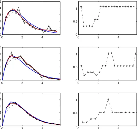
Figure 1. Scenario 1 with β = 1 andn= 500, ¯re = 1.02,pc = 0% (top),
n = 1000, ¯re = 1.04, pc = 0% (middle), n = 5000, ¯re = 0.97, pc = 0% (bottom)
5. Simulations
We illustrate the behavior of estimator ˇλ, constructed with the pointwise bandwidth selection of Section 4.1.
Recurrent events data are simulated as follows. For individualsi= 1, . . . , n, the terminal eventDi is simulated according to the distributionF, the censoring timeCi according to
G. Conditionally on Di, the number n(i) of recurrent events experienced by individual i
on time interval [0, Di] are simulated according to a Poisson distribution P(
RDi
0 ϕ(u)du). Finally the recurrent times for individual i is simulated as n(i) i.i.d. random variables with common p.d.fϕ/RD
0 ϕ(u)du. The intensity of the process N
∗ to recover is, in this
case, given by:
λ(t) =ϕ(t)(1−F(t)). We consider two scenarios for the simulated data:
(1) ϕ(t) =t and 1−F(t) = exp(−βt).
0 0.5 1 1.5 0 0.5 1 1.5 2 0 0.5 1 1.5 0 0.5 1 0 0.5 1 1.5 0 0.5 1 1.5 2 0 0.5 1 1.5 0 0.5 1 0 0.5 1 1.5 0 0.5 1 1.5 2 0 0.5 1 1.5 0 0.5 1
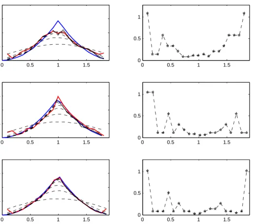
Figure 2. Scenario 2 with β = 0.05 and n = 500, ¯re = 0.92, pc = 0%
(top), n = 1000, ¯re = 0.89, pc = 0% (middle), n = 5000, ¯re = 0.91, pc= 0% (bottom)
The estimators of Section 4.1 are constructed with Epanechnikov kernels: K(t) = (3/4)(1−t2), if |t| ≤ 1. We use a data-driven criterion for the selection of the band-width, by replacingV0(h) in Definition (4) by:
ˆ V0(h) =κ0 ˆ cτkλˆk∞,τkKk2log(n) n hˆcG , with ˆ cτ = max i=1,...,n(t∈[0sup,T max] Ni(t)) + 2 kλˆk∞,τ = sup t∈[0,Tmax] |λ0ˆ .5(t)| and ˆ cG = 1−Gˆ(Tmax−),
The finite set of bandwidths (Hn) considered in the algorithm is given by:
Hn={log2(n)/n+ 1/2k, k = 0, . . . ,blog(n)/log(2)c}.
In the figures below, the intensity functions are estimated on a 20-points grid, regularly spaced on [0, Tmax] andκ0 equals 10−2. The number of observations n, the mean number of recurrent ¯re and the level of censoringpc are reported in the captions. In each figure, the left plots show the true intensity functions in red, the estimators in blue, and the set of all the estimators proposed to the selection algorithm is dashed black. The right plots show the value of the selected windows for all points on the grid.
In Figures 1 and 2, we investigate the behavior of our estimators, when the sample size ngrows. In scenario 1, where the intensity λto recover is smooth, as in scenario 2, where λhas a singularity, the estimator behaves as expected: it improves with the sample size.
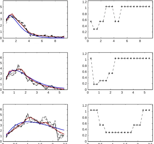
In Figure 3, we illustrate the behavior of our estimator when the censoring level grows. In this case, the censoring time has an exponential distribution, with 1−G(t) = exp(−γt), where the parameter γ takes the values γ = 1/30 (top), γ = 1/3 (middle) and γ = 1 (bottom). The resulting levels of censoring and mean numbers of recurrent events are indicated in the caption. Note that, as the level of the censoring grows, the numbers of observed recurrent events vanishes (from ¯re = 1.12, when pc = 4%, to ¯re = 0.25, whenpc= 50%) as does the time intervals, on which they are observed (from [0,9], when pc= 4%, to [0,2.5], when pc= 50%).
From a general point of view, we can see in Figures 1, 2 and 3 that the algorithm makes very different bandwidth choices, depending on the point of time. Therefore, the pointwise strategy is very useful. In particular, we can see in Figures 1 and 2 that the minimal bandwidth choice occurs at time 1 which in both cases is the location of the maximum; moreover, the selected bandwidth is all the smaller that the peak is abrupt. Lastly, Figure 3 shows that the pointwise strategy is relevant: indeed, it is obviously a good strategy to change the bandwidth in function of the time since none of the proposed curves would globally give a better estimate.
6. Concluding remarks
In this work, we not only provide a kernel estimator for the intensity function of a re-current event process, but we also prove oracle type inequalities for the risk of an adaptive estimator with data-driven selected bandwidth. We have studied both cases of pointwise risk for pointwise chosen bandwidth and integrated global risk with a globally selected bandwidth. Our bandwidth selection proposal is original and slightly different from stan-dard cross-validation methods. This is because it is based on recent ideas developed by Goldenshluger and Lepski [11]: in this sense, our results are new and the way of proving the results is of interest. We also assess the practical feasibility and the good performances of our proposal through a short simulation study: we found it more challenging to evaluate the pointwise selection and illustrate the different bandwidths choices performed by the algorithm.
0 2 4 6 8 0 0.1 0.2 0.3 0.4 0.5 0 2 4 6 8 0 0.2 0.4 0.6 0.8 1 1.2 0 1 2 3 4 5 0 0.1 0.2 0.3 0.4 0.5 0.6 0 1 2 3 4 5 0 0.2 0.4 0.6 0.8 1 1.2 0 0.5 1 1.5 2 2.5 0 0.1 0.2 0.3 0.4 0.5 0.6 0 0.5 1 1.5 2 2.5 0 0.2 0.4 0.6 0.8 1 1.2
Figure 3. Scenario 1 withβ = 1 andn= 1000, ¯re= 1.12,pc= 4% (top),
n = 1000, ¯re = 0.55, pc = 25% (middle), n = 1000, ¯re = 0.25, pc = 50% (bottom)
7. Proofs
7.1. Proof of Lemma 1. The proof relies on four additional lemmas which are presented below. First, write:
ˆ λh(t)−˜λh(t) = 1 nh n X i=1 Z ˆ G(s−)−G(s−) (1−Gˆ(s−))(1−G(s−))K t−s h dNi(s).
Then introduce the sets ΩG= n ω:∀t∈[0, τ], G(t)−Gˆ(t)≥ −cG/2 o , Ω?G=nω:∀t∈[0, τ],|G(t)−Gˆ(t)| ≤c0 p n−1logno, and (16) Ωc0 = ΩG∩Ω ? G.
Our idea is to study the difference process ˆλh−λ˜h on Ωc0 and its complementary. The
next lemma gives a useful bound ofP[Ωcc0]. The proof is postponed to Section 8.
Lemma 2. For all p∈N, there exists a choice of the constant c0=c0(p) such that,
(17) P h Ωcc 0(p) i ≤c2n−p,
where c2 is a constant depending on k, cF and cG andc0(k) also depends on cF.
In the following, we denote by Ωp = Ωc0(p) such that Equation (17) in Lemma 2 holds.
We now start the proof of Lemma 1 by studying the difference process ˆλh−λ˜h on the set
Ωcp.
Lemma 3. Under Assumptions 1 to 4, for all p∈N, t∈[h, τ−h], we have:
E h ˆ λh(t)−λ˜h(t) 2 I(Ωcp)i≤(n+ 1)2n2−p/2c3kKk2∞, where c3 =c3τ/2√c2 Z τ 0 λ(s)ds (1−G(s−))3 1/2 .
Consequently, choosingp≥10 yieldsE
h ˆ λh(t)−˜λh(t) 2 I(Ωcp) i
≤c/n for a positive con-stantc.
Lemma 4. Under Assumptions 1 to 4, for all p∈N, we have:
Z τ−h h E h ˆ λh(t)−˜λh(t) 2 I(Ωcp)idt≤(n+ 1)2n1−p/2c3kKk2.
Consequently, choosingp≥8yieldsRhτ−hE
h ˆ λh(t)−˜λh(t) 2 I(Ωcp) i dt≤c/nfor a positive constant c.
Proof of Lemmas 3 and 4. From the facts that 1−Gˆ(t) ≥ (n+ 1)−1 (see Equation (2)) andkGˆ−Gk∞<1, we have for allt∈[h, τ−h]:
E h ˆ λh(t)−λ˜h(t)2I(Ωcp) i ≤ (n+ 1) 2 n2 E n X i=1 Z Kh(t−s) 1−G(s−)dNi(s) !2 I(Ωcp) ≤(n+ 1)2E " Z K h(t−s) 1−G(s−)dN(s) 2 I(Ωcp) # ≤(n+ 1)2cτE " Z K2 h(t−s)I(Ωcp) (1−G(s−))2 dN(s) # , (18)
where the last inequality is obtained from Lemma 9. Now, for the proof of Lemma 3, use consecutively the Cauchy-Schwarz inequality and Lemma 9 to obtain:
E " Z K2 h(t−s)I(Ωcp) (1−G(s−))2 dN(s) # ≤E1/2 " Z K2 h(t−s) (1−G(s−))2dN(s) 2# q P[Ωcp] ≤ kKk2∞h−2√cτE1/2 Z τ 0 dN(s) (1−G(s−))4 q P[Ωcp] ≤ kKk2∞h−2n−p/2√c2cτ Z τ 0 λ(s)ds (1−G(s−))3 1/2 , and conclude the proof using the fact thath−1 ≤n. To prove Lemma 4 write,
Z τ−h h Z Kh2(t−s) (1−G(s−))2dN(s)dt≤ h −1kKk2 Z τ 0 dN(s) (1−G(s−))2. Then, using Cauchy-Schwarz inequality, we get from inequality (18):
Z τ−h h E h ˆ λh(t)−λ˜h(t) 2 I(Ωcp)idt≤ (n+ 1) 2c τ h kKk 2 E Z τ 0 I(Ωcp)dN(s) (1−G(s−))2 ≤ (n+ 1) 2 h cτkKk 2 E1/2 " Z τ 0 dN(s) (1−G(s−))2 2# q PΩcp ≤ (n+ 1) 2n−p/2 h c 3/2 τ √ c2kKk2 Z τ 0 λ(s)ds (1−G(s−))3 1/2 ,
and again, we conclude the proof using the fact thath−1 ≤n.
We now study the difference process of ˆλh−λ˜h on Ωp.
Lemma 5. Under Assumptions 1 to 4, we have for all t∈[h, τ−h]and any p∈N,
E h ˆ λh(t)−˜λh(t) 2 I(Ωp) i ≤ c4logn n kλk∞,τ kKk21kλk∞,τ + cτkKk2 cGnh , where c4= 4c20cG−2 and c0=c0(p). Consequently, for t∈[h, τ−h], we have
E h ˆ λh(t)−λ˜h(t) 2 I(Ωp) i ≤ clog(n) n ,
where c is a positive constant.
Lemma 6. Under Assumptions 1 to 4, we have, for any p∈N
Z τ−h h E h ˆ λh(t)−λ˜h(t) 2 I(Ωp) i dt≤ c4logn n kKk 2 2 Z τ 0 λ2(t)dt+cτΛ(τ) nh ,
where Λ(τ) is defined in Theorem 1. Consequently, we have
Z τ−h h E h ˆ λh(t)−λ˜h(t) 2 I(Ωp) i dt≤ clog(n) n ,
where c is a positive constant.
• 1−Gˆ(t) = 1−G(t) +G(t)−Gˆ(t)≥cG/2 on ΩG, • kG(t)−Gˆ(t)k∞≤c0 p n−1lognon Ω? G, to write: E h ˆ λh(t)−λ˜h(t) 2 I(Ωp) i ≤ 4c 2 0logn nc2G E 1 n n X i=1 Z |K h(t−s)| 1−G(s−)dNi(s) !2 . Then, we have: E " 1 n n X i=1 Z |K h(t−s)| 1−G(s−)dNi(s) #!2 = Z |Kh(t−s)|λ(s)ds 2 ≤ kKk2 1kλk2∞,τ, and V " 1 n n X i=1 Z | Kh(t−s)| 1−G(s−)dNi(s) # ≤ cτkKk 2kλk ∞,τ cGnh ,
which follows from Proposition 1. Combining these two bounds gives the final result of Lemma 5.
The proof of Lemma 6 follows the same line. From a change of variables and the Cauchy-Schwarz inequality we have:
Z τ−h h E " 1 n n X i=1 Z | Kh(t−s)| 1−G(s−)dNi(s) #!2 dt= Z τ−h h Z |Kh(t−s)|λ(s)ds 2 dt ≤ Z 1 −1 K2(u)du Z τ−h h Z 1 −1 λ2(t−uh)dudt ≤2kKk2 Z τ 0 λ2(t)dt,
where the last inequality was obtained from an other change of variables. On the other hand, from similar arguments as in the proof of Proposition 1, we have
Z τ−h h V " 1 n n X i=1 Z |K h(t−s)| 1−G(s−)dNi(s) # dt≤ cτΛ(τ) nh kKk 2,
and the result follows.
Gathering the results of Lemmas 3 to 6 imply the result of Lemma 1.
7.2. Proof of Theorem 2. First, for all h ∈ Hn, the following sequence of inequalities holds: ˇ λ(t0)−λ(t0)2 ≤3 ˆλˆh(t 0)(t0)− ˆ λh,ˆh(t0)(t0)2+ 3 ˆλh,ˆh(t0)(t0)−ˆλh(t0)2+ 3 ˆλh(t0)−λ(t0)2 ≤3 A0(h, t0) +V0(ˆh(t0))+ 3 A0(ˆh(t0), t0) +V0(h)+ 3 ˆλh(t0)−λ(t0)2 ≤6A0(h, t0) + 6V0(h) + 3 ˆλh(t0)−λ(t0) 2 .
Since V0(h), see (4), and (ˆλh(t0)−λ(t0))2, see Theorem 1, (i), have the adequate order (with additional log(n) forV0), we only studyA0(h, t0). With obvious definition of ˜λh,h0 =
Kh0∗˜λh,λh(t0) =E[˜λh(t0)] andλh,h0(t0) =E[˜λh,h0(t0)], A0(h, t0) can be decomposed into five terms: A0(h, t0) = sup h0∈H n n ˆ λh0(t0)−λˆh,h0(t0)2−V0(h0) o + ≤5 sup h0∈H n n ˜ λh0(t0)−λh0(t0)2−V0(h0)/10 o + + 5 sup h0∈H n n ˜ λh,h0(t0)−λh,h0(t0)2−V0(h0)/10 o + + 5 sup h0∈H n ˆ λh0(t0)−˜λh0(t0)2+ 5 sup h0∈H n ˆ λh,h0(t0)−λ˜h,h0(t0)2 + 5 sup h0∈H n λh0(t0)−λh,h0(t0)2 := 5(T0,1+T0,2+T0,3+T0,4+T0,5).
We start with the last one:
|λh0(t0)−λh,h0(t0)|=|Kh0∗λ(t0)−Kh0∗Kh∗λ(t0)|=|Kh0∗(λ−Kh∗λ)(t0)| ≤ kKk1 sup t∈[0,τ] |(λ−Kh∗λ)(t)|. This yields to T0,5 ≤ kKk21 kλ−Kh∗λk2∞,τ ≤ kKk21c21h2β,
sinceλ−Kh∗λcorresponds to the bias term in Proposition 1.
Then we decompose T0,3 into two terms corresponding toI(Ωp) andI(Ωcp) where Ωp is
defined by (16). First, from Lemma 3, we have
E sup h0∈H n (ˆλh0−λ˜h0)2(t0)I(Ωc p) ≤ X k,hk∈Hn E h (ˆλhk−λ˜hk) 2(t 0)I(Ωcp) i ≤ X k,hk∈Hn 4c3kKk2∞n4−p/2 ≤4c3kKk2∞n5−p/2,
using the fact that Card(Hn) ≤ n. Consequently, this term is of order 1/n as soon as
p≥12. On the other hand, the following sequence of inequalities holds:
E sup h0∈H n (ˆλh0−λ˜h0)2(t0)I(Ωp) ≤ 4c 2 0 c2 G log(n) n E sup h0∈H n Z | Kh0(t0−s)| 1−G(s−) 1 n n X i=1 dNi(s) !!2 ≤ 8c 2 0 c2G log(n) n E sup h0∈H n Z |K h0(t0−s)| 1−G(s−) 1 n n X i=1 dNi(s)−λ(s)(1−G(s−))ds !!2 +8c 2 0 c2G log(n) n hsup0∈H n Z |Kh0(t0−s)|λ(s)ds 2 ≤ 8c 2 0 c2 G log(n) n X k,hk∈Hn V " 1 n n X i=1 Z | Khk(t0−s)| 1−G(s−) dNi(s) # +8c 2 0kλk2∞,τ c2 G log(n) n kKk 2 1 ≤ 8c 2 0 c3 G log(n) n X k,hk∈Hn cτkλk∞,τkKk2 nhk +8c 2 0kλk2∞,τ c2 G log(n) n kKk 2 1, (19)
where the bound on the variance term comes from the proof of Proposition 1. Therefore
E[T0,3].log1+a(n)/n from Condition (8) and this ends the study ofT0,3.
The term T0,4 can be handled in a similar way using the relation ˆλh,h0(t0)−λ˜h,h0(t0) =
Kh0∗(ˆλh−λ˜h)(t0). Indeed, E sup h0∈H n (ˆλh,h0−˜λh,h0)2(t0)I(Ωcp) =E sup h0∈H n Kh0 ∗(ˆλh−λ˜h) 2 (t0)I(Ωcp) ≤ kKk21E h kλˆh−˜λhk2∞,τI(Ωcp) i ≤4c3kKk21kKk2∞n4−p/2,
from Lemma 3 and
E sup h0∈H n (ˆλh,h0 −λ˜h,h0)2(t0)I(Ωp) ≤ 8c 2 0 c2 G log(n) n X k,hk∈Hn V " 1 n n X i=1 Z | Khk∗Kh(t0−s)| 1−G(s−) dNi(s) # +8c 2 0 c2 G kλk∞,τ log(n) n hsup0∈H n kKh0∗Khk21.
Then, using the property
it is easy to see that V " 1 n n X i=1 Z |K hk∗Kh(t0−s)| 1−G(s−) dNi(s) # ≤ cτ ncG kλk∞,τkKh∗Khkk 2 ≤ cτ ncG kλk∞,τkKhk21kKhkk 2 ≤ cτkλk∞,τkKk 2 1kKk2 ncGhk , and kKh0∗Khk21 ≤ kKh0k21kKhk21=kKk41.
We conclude as previously thatE[T0,4].log1+a(n)/n.
Finally, let us study the terms T0,1 and T0,2. We start by recalling the following con-centration inequality.
Lemma 7. [Bernstein inequality] Let ξ1, . . . , ξn be independent and identically distributed
random variables and Sn(ξ) =Pni=1ξi. Then, for η >0,
(21) P(|Sn(ξ)−E[Sn(ξ)]| ≥nη)≤2 max exp −nη 2 4w ,exp −nη 4b ,
where w andb are such that |ξ1| ≤b almost surely and V(ξ1)≤w. Now, we want to apply this result to ξi =
R
Kh(t0−s)dNi(s)/(1−G(s−)). First, we
need to establish the values of the boundsb and w. We have
|ξ1| ≤(cτkKk∞)/(cGh) :=band V(ξ1)≤cτkλk∞,τkKk2/(cGh) :=w.
Thus, Inequality (21) can be written in the following way: for somex >0,
P h |λ˜h(t0)−λh(t0)| ≥ p V0(h)/10 +x i
≤2 maxexp(−n(V0(h)/10 +x)/(4w)),exp(−n p
V0(h)/10 +x/(4b))
≤2 max
exp(−n(V0(h)/10 +x)/(4w)),exp(−npV0(h)/5/(8b)) exp(−npx/2/(4b))
. Then, we setκ0≥80, in order to have
nV0(h)
40w = (κ0/40) log(n)≥2 log(n). On the other hand,
npV0(h) 8b√5 = kKkp cGκ0kλk∞,τ 8kKk∞ √ 5cτ p nhlog(n) :=κ2pnhlog(n).
Then takingκ1 ≥4κ−22 in Condition (7) gives, npV0(h) 8b√5 ≥2 log(n). Therefore, we have P h |λ˜h(t0)−λh(t0)| ≥ p V0(h)/10 +x i ≤2n−2maxe−κ3nhx, e−κ4nh √ x,
where κ3= cG 4cτkλk∞,τkKk2 and κ4 = cG 4cτkKk∞ √ 2. This yields E n |˜λh(t0)−λh(t0)|2−V0(h)/10 o + ≤ Z +∞ 0 P h |λ˜h(t0)−λh(t0)| ≥ p V0(h)/10 +x i dx ≤2n−2max Z +∞ 0 e−κ3nhxdx, Z +∞ 0 e−κ4nh √ xdx ≤2n−2max 1 κ3nh , 2 κ2 4(nh)2 ≤κ5n−2,
for some positive constantκ5. Finally,
E[T0,1] =E sup h0∈H n n ˜ λh0 −λh02(t0)−V0(h0)/10 o + ≤ X k,hk∈Hn E n ˜ λhk−λhk 2 (t0)−V0(hk)/10 o + ≤κ5 Card(Hn)n−2,
and since Card(Hn)≤n, we conclude that E[T0,1].n−1.
The last term is T0,2 which can be treated in a similar way. Write
E[T0,2] =E sup h0∈H n n ˜ λh,h0−λh,h02(t0)−V0(h0)/10)+ o ≤ X k,hk∈Hn E n ˜ λh,hk−λh,hk 2 (t0)−V0(hk)/10 o + .
Then the sequel is the same as for the proof of T0,1 except that all h vanish because
kKh∗Kh0k∞≤ kKh0k∞kKk1.
Gathering the bounds of the five terms gives the result of Theorem 2.
7.3. Proof of Theorem 3. Following the lines of the proof of Theorem 2, we have, for allh∈ Hn,
kλ∗−λk2 ≤3kλˆˆh−λˆh,hˆk2+ 3kλˆh,ˆh−ˆλhk2+ 3kλˆh−λk2
≤3(A(h) +V(ˆh)) + 3(A(ˆh) +V(h)) + 3kˆλh−λk2
≤6A(h) + 6V(h) + 3kˆλh−λk2.
Here again,V(h) andkλˆh−λk2(see Theorem 1, (ii)) have the adequate order and we only
and write: A(h) = sup h0∈H n n kˆλh0 −λˆh,h0k2−V(h0) o + ≤5 sup h0∈H n n k˜λh0 −λh0k2−V(h0)/10 o ++ 5 suph0∈H n n k˜λh,h0 −λh,h0k2−V(h0)/10 o + + 5 sup h0∈H n kλˆh0−˜λh0k2+ 5 sup h0∈H n kˆλh,h0−λ˜h,h0k2+ 5 sup h0∈H n kλh0−λh,h0k2 := 5(T1+T2+T3+T4+T5). We start withT5: kλh0−λh,h0k2 =kKh0∗(λ−Kh∗λ)k2 ≤ kKh0k2 1kλ−Kh∗λk2,
where we used the property (20) withq= 2. This yields to T5 ≤ kKk21τ c21h2β,
sincekλ−Kh∗λk corresponds to the bias term in Proposition 1.
Now, the same kind of arguments can be applied to T4: ˆ λh,h0−˜λh,h0 =Kh0∗(ˆλh−λ˜h), and so, E[T4]≤ kKk21E h kˆλh−λ˜hk2 i ≤c0kKk21log(n)/n, where the last inequality was obtained from Lemma 1.
The termT3 can be dealt with in the same way asT0,3 in the proof of Theorem 2. First, from Lemma 4, E sup h0∈H n Z (ˆλh0 −λ˜h0)2(t)I(Ωc p)dt ≤ X j,hj∈Hn Z E[(ˆλhj−˜λhj) 2(t)I(Ωc p)]dt ≤ X j,hj∈Hn 4c3kKk2n3−p/2≤4c3kKk2n4−k/2,
and this term is of order 1/nas long as p≥10. Then, using similar inequalities as in (19) yields E sup h0∈H n Z τ−h h (ˆλh0 −λ˜h0)2(t)I(Ωp)dt ≤ 8c 2 0 c2 G log(n) n X k,hk∈Hn cτΛ(τ)kKk2 nhk + 16c 2 0 c2 G log(n) n kKk 2 Z τ 0 λ2(t)dt,
and we conclude from Equation (8) thatE[T3].loga+1(n)/n.
We finish the proof with T1 and T2. As in Theorem 2, these two terms can be treated using a concentration inequality. First, we need to express each of them as a centered
empirical process. ForT1, write E " sup h0∈H n kλ˜h0−λh0k2−V(h0)/10 + # ≤ X k,hk∈Hn E n kλ˜hk −λhkk 2−V(h k)/10 o + , and recall that
(22) kλ˜hk −λhkk
2= sup
f∈L2([hk,τ−hk]),kfk=1
h˜λhk −λhk, fi
2.
Now, we introduce the following centered empirical process: νn,hk(f) =hλ˜hk−λhk, fi= 1 n n X i=1 Z τ−hk hk f(u) Z Khk(u−s) dNi(s) 1−G(s−) −λ(s)ds du. Asf 7→νn,hk(f) is continuous, the supremum in (22) can be taken over a countable dense
subset of{f ∈L2([1, τ −1]),kfk= 1}, which we denote by Bτ(1). Therefore,
E[T1]≤ X k,hk∈Hn E "( sup f∈Bτ(1) νn,h2 k(f)−V(hk)/10 ) + #
and the expectation here can be bounded using the following concentration inequality.
Theorem 4. (Talagrand Inequality) Let ξ1, . . . , ξn be independent random values, and
let νn,ξ(f) = (1/n)Pni=1{f(ξi)−E[f(ξi)]}. Then, for a countable class of functions F
uniformly bounded andε >0, we have E " n sup f∈F νn,ξ2 (f)−2(1 + 2ε2)H2 o + # ≤ 4 d W ne −dε2nH2 W + 98M 2 dn2ϕ2(ε)e −2dϕ(ε)ε 7√2 nH M , withϕ(ε) =√1 +ε2−1,d= 1/6 and sup f∈F kfk∞≤M, E h sup f∈F |νn,ξ(f)| i ≤H, sup f∈F 1 n n X i=1 V[f(ξi)]≤W.
To apply this result, we first need to compute appropriate values of the bounds H,M, W and the constant ε. Clearly,
E " sup f∈Bτ(1) νn,h2 k(f) # ≤E h kλ˜hk−λhkk 2i= Z τ−hk hk V h ˜ λhk(t) i dt=V(hk)/κ
and thus we require H2 =V(hk)/κ. Then we set ε2 = 1/2 andκ = 40 in order to have
2(1 + 2ε2)H2 =V(h
k)/10.
Now to find the boundM, use the Cauchy-Schwarz inequality and the fact thatkfk= 1 onBτ(1) to write: Z τ−hk hk f(u) Z Khk(u−s) dN(s) 1−G(s−)du = Z Z τ−hk hk f(u)Khk(u−s)du dN(s) 1−G(s−) ≤ kfk Z Z τ−hk hk Kh2k(u−s)du 1/2 dN(s) 1−G(s−) ≤ cτkKk cG 1 √ hk :=M.
Lastly, we need to determine the adequate bound W. Introduce the notation Kh− k(s) = Khk(−s) and write: V Z τ−hk hk f(u) Z Khk(u−s) dN(s) 1−G(s−)du ≤E " Z Z τ−hk hk Khk(u−s)f(u)du dN(s) 1−G(s−) 2# ≤E " Z Kh− k∗f(s) dN(s) 1−G(s−) 2# ≤cτ Z (K− hk ∗f) 2(s) 1−G(s−) λ(s)ds ! ≤ cτkλk∞,τ cG kKh− k∗fk 2 ≤ cτkλk∞,τ cG kKh− kk 2 1kfk2 = cτkλk∞,τkKk21 cG :=W,
where we used Lemma 9 and the property (20) forq = 2. Therefore, W is a constant and we can now apply Talagrand Inequality:
E "( sup f∈Bτ(1) νn,h2 k(f)−V(hk)/10 ) + # ≤ ϑ1 n exp(−ϑ2/hk) + 1 nhk exp(−ϑ3√n) ,
for some positive constants ϑ1, ϑ2 and ϑ3. Then, from conditions (8), (14) and the fact that Card(Hn)≤n, we conclude:
E[T1]≤ ϑ1 n X k,hk∈Hn exp(−ϑ2/hk) + 1 nhk exp(−ϑ3 √ n) . 1 n.
The proof for T2 follows the same line as for T1. First,
E[T2]≤ X k,hk∈Hn E n k˜λh,hk −λh,hkk 2−V(h k)/10 o +
and the Talagrand inequality needs to be applied to the centered processhλˆh,hk−λh,hk, fi,
where f ∈ Bτ(1). Since ˜λh,hk = Kh∗˜λhk and λh,hk =Kh∗λhk the same bounds H, M
andW can be used, up to a constant. Indeed, using the inequalities
kKh∗Khkk2 ≤ kKk1kKk2(hk)
−1/2 and kK
h∗Kh−kk1≤ kKk21 it can be shown that Theorem 4 can be applied with
H2= V(hk)kKk 2 1 κ , M = cτkKk1kKk cG √ hk and W = cτkλk∞,τ cG kKk41.
Finally, we obtain againE[T2].1/n.
8. Technical lemmas
In order to give a proof of Lemma 2, we first need to introduce the following result which is a direct consequence of Theorem 1 in [4].
Lemma 8. For all k∈N∗, there exists a positive constant c
k depending on k such that
E
h
kGˆ−Gk2∞,τk i≤ ck
nk.
Proof. We use a nonasymptotic exponential bound for the Kaplan-Meier estimator which can be formulated as follows (see Bitouz´e et al., [4]): there exists a positive constant η such that for any positive constantε,
(23) P h√ nk(1−F) ( ˆG−G)k∞,τ > ε i ≤2.5e−2ε2+ηε and so E h kGˆ−Gk2∞,τk i ≤2k Z +∞ 0 u2k−1P h kGˆ−Gk∞,τ > u i du ≤2k Z +∞ 0 u2k−1P h c−F1k(1−F) ( ˆG−G)k∞,τ > u i du ≤2k Z +∞ 0 u2k−1P h√ nk(1−F) ( ˆG−G)k∞,τ > cF √ n uidu ≤5keη2/8 Z ∞ 0 u2k−1exp ( −2c2Fn u− η 4√ncF 2) du ≤ 5e η2/8 k 2kc2k F Z +∞ −η/(2√2) z+ η 2√2 2k−1 e−z2dz n−k:=ckn−k.
Proof of Lemma 2. Since P[Ωc]≤ P[ΩcG] +P[(Ω?G)c], we bound each term separately.
For anyk >0, we have
P[ΩcG]≤P h kG−Gˆk∞,τ > cG/2 i ≤ 4 k c2k G E h kG−Gˆk2k ∞,τ i . Thus, Lemma 8 implies that
(24) P[ΩcG]≤dkn−k, wheredk >0.
Next, we use (23) and write:
P h kGˆ−Gk∞,τ > c0 p n−1log(n)i ≤Phk(1−F)(y) ˆG−Gk∞,τ > c0cF p n−1log(n)i ≤2.5 exp(−2c2Fc20log(n) +ηcFc0 p
Thus, forc0≥(η+pη2+ 8k)(4c F)−1 we have P[Ω?cG] =P h kG−Gˆk∞,τ > c0 p n−1logni≤2.5n−k.
This result and Equation (24) implyP[Ωc]≤(dk+ 2.5)n−k.
We conclude this section with a very useful inequality concerning integrals with respect to the counting processN.
Lemma 9. (Cauchy-Schwarz) For every bounded function h on [0, τ], we have
N(τ) Z τ2 τ1 h2(s)dN(s)≥ Z τ2 τ1 h(s)dN(s) 2 , where 0≤τ1≤τ2 ≤τ. Proof. We have 0≤ Z τ2 τ1 h(s)− Z τ2 τ1 h(s)dN(s) N(τ) 2 dN(s) N(τ) 0≤ 1 N(τ) Z τ2 τ1 h2(s)dN(s)−2 Z τ2 τ1 h(s)dN(s) N(τ) 2 + Z τ2 τ1 h(s)dN(s) N(τ) 2Z τ2 τ1 dN(s) N(τ).
Then, notice thatRτ2
τ1 dN(s)≤N(τ) to obtain the desired result.
References
[1] P. K. Andersen, Ø. Borgan, R. D. Gill, and N. Keiding.Statistical models based on counting processes. Springer Series in Statistics. Springer-Verlag, New York, 1993.
[2] P. K. Andersen and R. D. Gill. Cox’s regression model for counting processes: a large sample study.
Ann. Statist., 10(4):1100–1120, 1982.
[3] R. Bartoszy´nski, B. W. Brown, C. M. McBride, and J. R. Thompson. Some nonparametric techniques for estimating the intensity function of a cancer related nonstationary Poisson process.Ann. Statist., 9(5):1050–1060, 1981.
[4] D. Bitouz´e, B. Laurent, and P. Massart. A Dvoretzky-Kiefer-Wolfowitz type inequality for the Kaplan-Meier estimator.Ann. Inst. H. Poincar´e Probab. Statist., 35(6):735–763, 1999.
[5] O. Bouaziz, Geffray S., and O. Lopez. Semi-parametric inference for the recurrent event process by means of a single-index model.arXiv:1005.4553, 2010.
[6] C.-T. Chiang, M.-C. Wang, and C.-Y. Huang. Kernel estimation of rate function for recurrent event data.Scand. J. Statist., 32(1):77–91, 2005.
[7] J.-Y. Dauxois and S. Sencey. Non-parametric tests for recurrent events under competing risks.Scand. J. Stat., 36(4):649–670, 2009.
[8] D. Ghosh and D. Y. Lin. Nonparametric analysis of recurrent events and death.Biometrics, 56(2):554– 562, 2000.
[9] D. Ghosh and D. Y. Lin. Marginal regression models for recurrent and terminal events.Statist. Sinica, 12(3):663–688, 2002.
[10] D. Ghosh and D. Y. Lin. Semiparametric analysis of recurrent events data in the presence of dependent censoring.Biometrics, 59(4):877–885, 2003.
[11] A. Goldenshluger and O. Lepski. Bandwidth selection in kernel density estimation: oracle inequalities and adaptive minimax optimality.The Annals of Statistics, 39(3):1608–1632, 2011.
[12] A. Goldenshluger and O. Lepski. Uniform bounds for norms of sums of independent random functions.
The Annals of Probability, to appear., 2011.
[13] J. F. Lawless and C. Nadeau. Some simple robust methods for the analysis of recurrent events. Tech-nometrics, 37(2):158–168, 1995.
[14] D. Y. Lin, L. J. Wei, I. Yang, and Z. Ying. Semiparametric regression for the mean and rate functions of recurrent events.J. R. Stat. Soc. Ser. B Stat. Methodol., 62(4):711–730, 2000.
[15] S. H. Lo, Y. P. Mack, and J. L. Wang. Density and hazard rate estimation for censored data via strong representation of the Kaplan-Meier estimator.Probab. Theory Related Fields, 80(3):461–473, 1989. [16] W. Nelson. Confidence limits for recurrence data – applied to cost or number of product repairs.
Technometrics, 37(2):147–157, 1995.
[17] M. Pepe and J. Cai. Some graphical displays and marginal regression analyses for recurrent failure times and time dependent covariates.J. Amer. Statist. Assoc., 88(423):811–820, 1993.
[18] A. B. Tsybakov.Introduction to nonparametric estimation. Springer Series in Statistics. Springer, New York, 2009. Revised and extended from the 2004 French original, Translated by Vladimir Zaiats.