Civil Engineering Journal
Vol. 4, No. 5, May, 2018Comparison of Three Intelligent Techniques for Runoff Simulation
Mahsa H. Kashani
a*,
Reza Soltan Gheys
baDepartment of Water Engineering, Faculty of Agriculture and Natural Resources, University of Mohaghegh Ardabili, Ardabil, Iran. bGraduated in IT Engineering, Company of Arman Tarh Farda, Tehran, Iran.
Received 11February2018; Accepted 25March2018
Abstract
In this study, performance of a feedback neural network, Elman, is evaluated for runoff simulation. The model ability is compared with two other intelligent models namely, standalone feedforward Multi-layer Perceptron (MLP) neural network model and hybrid Adaptive Neuro-Fuzzy Inference System (ANFIS) model. In this case, daily runoff data during monsoon period in a catchment located at south India were collected. Three statistical criteria, correlation coefficient, coefficientof efficiencyand the difference of slope of a best-fit line from observed-estimated scatter plots to 1:1 line, were applied for comparing the performances of the models. The results showed that ANFIS technique provided significant improvement as compared to Elman and MLP models. ANFIS could be an efficient alternative to artificial neural networks, a computationally intensive method, for runoff predictions providing at least comparable accuracy. Comparing two neural networks indicated that, unexpectedly, Elman technique has high ability than MLP, which is a powerful model in simulation of hydrological processes, in runoff modeling.
Keywords:Elman; MLP; ANFIS; Runoff Simulation;India.
1. Introduction
The short-term and long-term simulations of runoff is of vital interest in management of water resources projects and also watershed management that includes increasing infiltration into soil, controlling excess runoff, managing and utilizing runoff for specific purposes, and reducing soil erosion. The non-linear and complex nature of the runoff process, its variability depending on catchment characteristics and precipitation patterns, and its dependence on various other factors make it difficult to predict and estimate runoff with desirable accuracy. However, over the years, hydrologists have developed several models ranging from empirical relationships to physically-based. The physically-based models have proved to be better for the simulation of runoff, but their data requirements are very high and often intensively-monitored watersheds lack sufficient input data for these models. Therefore, the need to develop alternative models to simulate runoff using available data has taken priority. Recently, pattern-recognition algorithms such as the artificial neural networks (ANN) have gained popularity in simulating the rainfall-runoff processes producing comparable accuracy to those of the physically-based models [1-3].
The theory of Artificial Neural Networks (ANNs) started in early 1940’s when the first computational representation of a neuron was developed by McCulloch and Pitts [4]. Basically, ANNs is one of Artificial Intelligence techniques that mimic the behavior of the human brain. In the last decade, ANNs have been successfully employed in modeling a wide range of hydrologic processes, including rainfall–runoff processes; Smith and Eli [5]; Hsu et al [6]; Minns and Hall [7]; Shamseldin [8] and Dawson and Wilby [9] studied on neural-network models of rainfall–runoff process. Tokar and Johnson [10] developed an ANN model to predict daily runoff as a function of daily precipitation, temperature, and
* Corresponding author: [email protected] http://dx.doi.org/10.28991/cej-0309159
This is an open access article under the CC-BY license (https://creativecommons.org/licenses/by/4.0/). © Authors retain all copyrights.
snowmelt for a watershed in Maryland, USA. Chiang et al [11] compared the static-feed forward and dynamic-feedback neural networks for rainfall–runoff modeling. Tayfur and Singh [12] used ANN and fuzzy logic models for simulating event-based rainfall–runoff. Tayfur et al [13] presented a model to predict and forecast flow discharge at sites receiving significant lateral inflow. Abudu et al. [14] forecasted monthly streamflow using autoregressive integrated moving average (ARIMA), seasonal ARIMA (SARIMA), and Jordan-Elman artificial neural networks (ANN) models over the Kizil River in Xinjiang, China. Tampelini et al. [15] presented the application of Elman neural network for rainfall-runoff simulation in Brazil. Sarkar and Kumar [16] modeled the event-based rainfall-rainfall-runoff process using the ANN technique over the Ajay River basin. Hasanpour Kashani et al. [17] evaluated capacity of the ANN [multilayer perceptron (MLP)] and Volterra model to approximate arbitrary non-linear rainfall–runoff processes in north of Iran. Devi et al. [18] adopted different ANN models for daily rainfall prediction using two different data sets in Nilgiris.
Although ANN is quite powerful for modeling various real world problems, it also has its shortcomings. If the input data are less accurate or ambiguous, ANN would be struggling to handle them and a fuzzy system such as Adaptive Neuro-Fuzzy Inference System (ANFIS) might be a better option. Jang [19] first proposed the ANFIS method and applied its principles successfully to many problems. Fundamentally, ANFIS is a network representation of Sugeno-type fuzzy systems, endowed by neural learning capabilities. Vernieuwe et al [20] used different clustering algorithms to identify Takagi–Sugeno models in a data-driven manner. The ANFIS technique has been successfully applied in many different hydrologic studies. Gautam and Holz [21] explored the applicability and effectiveness of ANFIS models for both forecasting and simulating the rainfall-runoff process in the Sieve basin in Italy. Lee and Han [22] compared the potentials of different neurofuzzy models for simulating real-time flood forecasting applications. Akrami et al. [23] applied the wavelet decomposition method to link to ANFIS and ANN models for enhancing the accuracy of rainfall prediction at Klang Gates Dam. Wahyuni et al. [24] used the Genetic Algorithm for optimizing the Sugeno FIS of the ANFIS model in boundaries of membership function and coefficient consequent rule in order to predict rainfall with the smallest error over the Tengger Indonesia.
The main objective of this article is to analyze the ability of a feedback ANN model, Elman, and compare its performance with a feedforward Multi-Layer Perceptron neural network (MLP) and ANFIS technique in simulating daily runoff data series over an Indian watershed.
2. Methods and Materials
2.1. Artificial Neural Networks 2.1.1. Multi-Layer Perceptron (MLP)
Most ANNs such as Multi-Layer Perceptron (MLP) networks have three layers or more: an input layer, which is used to present data to the network; an output layer, which is used to produce an appropriate response (s) to the given input; and one or more intermediate layers, which are used to act as a collection of feature detectors (Figure 1). The ability of a neural network to process information is obtained through a learning process, which is the adaptation of link weights so that the network can produce an approximate output (s). In general, the learning process of an ANN will reward a correct response of the system to an input by increasing the strength of the current matrix of nodal weights. There are several features in ANN that distinguish it from the empirical models. First, neural networks have flexible nonlinear function mapping capability which can approximate any continuous measurable function with arbitrarily desired accuracy, whereas most of the commonly used empirical models do not have this property. Second, being nonparametric and data-driven, neural networks impose few prior assumptions on the underlying process from which data are generated. Because of these properties, neural networks are less susceptible to model misspecification than most parametric nonlinear methods. Given the advantages of neural networks, it is not surprising that this methodology has attracted overwhelming attention in many application areas. However, it may take a lot of time for determining the best structure of the ANN model for a problem because of applying the trial and error method. There are a wide variety of algorithms available for training a network and adjusting its weights. Also, there are many kinds of neural networks. In this paper, MLP and Elman networks were applied. Since there are large number of resources available on ANN and MLP (books, papers and web sites), no further introduction is provided here and readers are referred to Haykin [25].
The operation process of MLP networks is so that the input layer accepts the data and the intermediate layer processes them and finally the output layer displays the resultant outputs of the model. During the modeling stage, coefficients related to present errors in nodes are corrected through comparing the model outputs with recorded input data. Connection weights are first initialised randomly by assigning a small positive or negative random value through the following procedure:
1. Input–output patterns are selected randomly using the training data presented to ANN.
2. Actual network outputs are calculated for the current input after the application to the activation function. 3. Performance measure is selected, e.g. Mean Square Error (MSE) and the values are calculated.
4. Connection weights are adjusted to minimise the MSE.
5. Steps (2)–(5) are repeated for each pair of input–output vector in the training datasets, until no significant change in the MSE is detected for the system.
The final connection weights are kept fixed at the completion of training and new input patterns are presented to the network to produce the corresponding output consistent with the internal representation of the input/output mapping [26].
Figure 1. MLP network
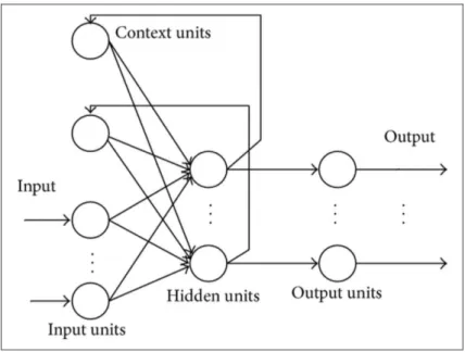
2.1.2. Elman Network
Elman Networks are a form of recurrent Neural Networks which have connections from their hidden layer back to a special copy layer (Figure 2). This means that the function learnt by the network can be based on the current inputs plus a record of the previous state (s) and outputs of the network. In other words, the Elman net is a finite state machine that learns what state to remember (i.e., what is relevant). The special copy layer is treated as just another set of inputs and so standard back-propagation learning techniques can be used (something which isn't generally possible with recurrent networks). At each time step, a copy of the hidden layer units is made to a copy layer [27].
Because Elman networks are an extension of two-layer Sigmoid-Linear architecture [25, 28], they inherit the ability to fit any input/output function with a finite number of discontinuities. They are also able to fit temporal patterns, but may need many neurons in the recurrent layer to fit a complex function. Also because of the more complex architecture of the recurrent model, there is a significant increase in training time compared with the MLP model [29].
2.2. Adaptive Neuro-Fuzzy Inference System (ANFIS)
The Adaptive Neuro-Fuzzy Inference System (ANFIS) is a universal approximator firstly introduced by Jang [19] that is capable of approximating any real continuous function on a compact set to any degree of accuracy [30]. ANFIS network is comprised of nodes and with specific functions, or duties, collected in layers with specific functions [31]. It identifies a set of parameters through a hybrid learning rule combining the back-propagation gradient descent error digestion and a least-squares method. It can be used as a basis for constructing a set of fuzzy “If–Then” rules with appropriate membership functions in order to generate the preliminary stipulated input–output pairs. The Gaussian membership function is adopted in this study since it is the most popular form. An ANFIS toolbox from Matlab software is used and its operation is explained in its user guide. For its theoretical background, interested readers are referred to Chang and Chang [32] for further details.
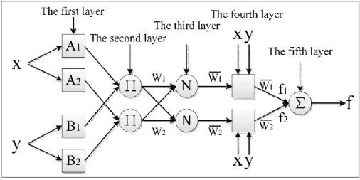
Figure 3 represents a typical ANFIS architecture, and outline as follows:
Layer 1: Every node in this layer is an adaptive node with a node function that may be a generalised bell membership function or a Gaussian membership function.
Layer 2: Every node in this layer is a fixed node labelled, P, representing the firing strength of each rule, and is calculated by the fuzzy AND connective of the ‘product’ of the incoming signals.
Layer 3: Every node in this layer is a fixed node labelled N, representing the normalised firing strength of each rule. The ith node calculates the ratio of the ith rule’s firing strength to the sum of two rules’ firing strengths.
Layer 4: Every node in this layer is an adaptive node with a node function indicating the contribution of ith rule toward the overall output.
Layer 5: The single node in this layer is a fixed node labelled, R, indicating the overall output as the summation of all incoming signals.
The above comprise three different types of components, as follows [33]:
1. Premise parameters as non-linear parameters that appear in the input membership functions. 2. Consequent parameters as linear parameters that appear in the rules consequents (output weights). 3. Rule structure that needs to be optimised to achieve a better linguistic interpretability [26].
Figure 3. A typical ANFIS architecture
3. Study Area and Data Sets
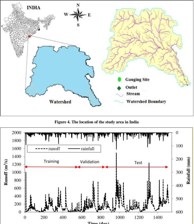
The study area chosen for this study is the Vamsadhara river basin, situated in between the Mahanadi and Godavari river basins of south India (Figure 4). The area is located between 18º15’ to 19º55’ north latitudes and 83º20’ to 84º20’ east longitudes. The precipitation in the basin is influenced by the occasional cyclones formed due to the depression in the Bay of Bengal and the south-west monsoon from June to October. The basin has six rain gauge stations and the weighted rainfall for the study area was estimated using the Thiessen polygons.
The rainfall and runoff data of monsoon period (June 1-October 31) for 1984-87 was used for training the ANNs and ANFIS models, and the data of 1988-89 and 1992-95 for their validation and testing (Figure 5). Some statistical parameters of the used data for three periods are shown in Table 1.
Figure 4. The location of the study area in India
Figure 5. Observed rainfall and runoff data
Table 1. Statistical parameters of the used data for three periods Statistical parameters
Data Period Average Standard deviation Maximum Minimum Mode
Rainfall Training 6.184 10.399 89.76 0 0 Validating 6.765 9.982 63.19 0 0 Testing 7.125 12.801 126.3 0 0 Runoff Training 94.428 109.450 994.4 0.5 32 Validating 149.357 134.861 772 0.5 65 Testing 198.935 196.959 1470 0 68.8 0 100 200 300 400 500 600 0 200 400 600 800 1000 1200 1400 1600 1800 2000 0 200 400 600 800 1000 1200 1400 R ai n fal l (m m ) R u n o ff (m 3/s ) Time (day) runoff rainfall Test Validation Training
4. Performance Criteria
The comparative analysis and evaluation of the outcome of the models was done using correlation coefficient (r), coefficient of efficiency (E), and the difference of slope (SDiff). Out of all the various performance measures, in the past the most widely used evaluation for the validation of models is the correlation-based measures i.e. the r and R2. However,
they suffer from several limitations such as insensitivity towards additive and proportional difference occurring between the observed and the predicted data, and the over-sensitivity to outliers leading to a bias towards extreme events [34]. These limitations of the correlation-based measures are well documented [34-38].
Coefficient of efficiency (E) is a non-dimensional criterion proposed by Nash and Sutcliffe [39] and widely used to evaluate the performance of hydrologic models. E = 100 indicates a perfect agreement between the observed and the estimated values. E = 0 indicates that all the estimated values are equal to the mean of the observed values. A negative E indicates that the mean of the observed data is a better predictor than the estimated values. The coefficient of efficiency was an improvement over the correlation-based measures because it is sensitive to the observed and predicted means and variances but is also limited in the case of over-sensitivity to outliers [34, 39].
The idea behind using SDiff is that while r is used to indicate the variational accountability of a model and E the efficiency, there is no comparative measure for the degree of predictability of a best-fit model to the 1:1 line when observed vs. predicted values are compared to each other. Hence, we have used SDiff as a measure of how different the slope of a best-fit line of the scatter plot of the predicted vs. observed data for a particular model is from the 1:1 line. SDiff of 0% means the best-fit line of a scatter plot is parallel to the 1:1 line thus ensuring perfect predictability of the best-fit linear model. SDiff of 100% means the best-fit line is the average line with a zero slope. SDiff between 0% and
100% would suggest that the best-fit linear model of the scatter plot would overestimate the low observed values and underestimate the high ones. A negative SDiff measure would suggest that the best-fit linear model of the scatter plot would underestimate the low observed values and overestimate the high ones.
5. Results and Discussions
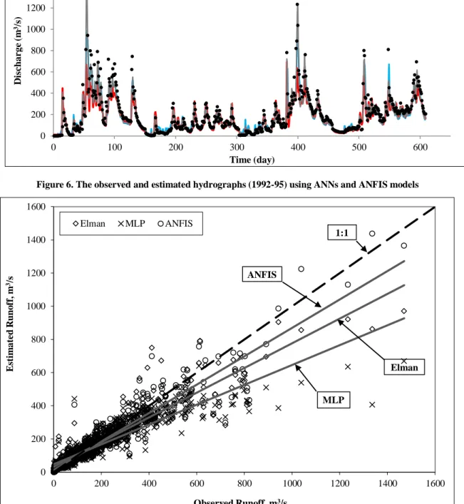
In order to obtain daily estimates of runoff using ANNs (MLP and Elman) and ANFIS approaches, 4 years of rainfall and runoff data (1984-87) was used to train the models and 2 years of data (1988-89) was used for validating to ensure similar model performance. Then the models were tested by estimating 4 years of future data (1992-95). We believe that different sets of input parameters that make hydrological sense for runoff estimation might improve performance accuracy of the models, which was beyond the scope of this paper due to our comparative analysis with of the applied models. First, different combinations of delayed rainfall and runoff data were used as the models inputs. Finally, it was found that rainfall at the current day and one day ago along with the runoff values at the current day, one day and two days ago are the best input variables for estimating the current runoff values. The data were normalized before applying the ANNs methods. The observed and estimated data of period 1992-95 were compared using r, E, and SDiff performance evaluation measures. The statistical criteria values obtained for the models at test and validation periods are presented at Table 1. The coefficients of correlation for the models MLP, Elman and ANFIS for validation period are 0.90, 0.93, and 0.95, respectively. These high values of r show that all the models are suitable for runoff simulation. The coefficient of efficiency (E) values of the models are almost high (0.727, 0.839 and 0.888), which shows good ability of the models in runoff prediction. However, ANFIS and Elman are more suitable based on high values of E, respectively. The SDiff values indicate that ANFIS has the lowest value (14.35%). The SDiff value of Elman (25.53%) is lower than that of MLP (40.15%). Therefore, ANFIS and Elman methods are more successful than MLP according to the SDiff values.
Figure 6 indicates the predicted hydrographs using the applied models versus the observed hydrograph. According to this figure, it can be found that the ANFIS model predicted the low and high flow values more successfully than the ANNs. Moreover, performance of the Elman technique in estimating flow values especially peak discharges is better than the MLP. Figure 7 shows the scatter plot of the estimated runoff versus the observed runoff data. It is evident from Figure 7 that the line related to ANFIS and Elman data points are closer to line 1:1. This indicates that ANFIS and Elman estimations are close to the observed data series, respectively. The line related to the MLP data points is far from the line 1:1 and indicates poor performance of MLP. Generally, as it is expected the hybrid ANFIS model estimated runoff values with high accuracy than the ANNs. The studies done by Gautam and Holz [21] and Lee and Han [22] proved that ANFIS is a power tool for time series predictions. However, Khatibi et al. [26] indicated that MLP simulates single-peaked flow time series with less error that the ANFIS.
The results of the feedback Elman network were more precise than those of MLP model, which has shown successful performances in different hydrological studies. The results obtained from the MLP model is in agreement with those of the study done by Misra et al. [40] who found that MLP is not successful in precisely daily runoff modeling. It can be concluded that feedback networks due to their structures are more able than feedforward networks in modeling processes with high nonlinearity such as daily runoff process. Abudu et al. [14] and Tampelini et al. [15] found that the Elman
6.
Conclusion
This paper gives an overview of fairly recent AI techniques on the topic of runoff estimating from an Indian watershed. In this case, two feed-forward and feed-back neural networks, MLP and Elman, along with the hybrid.
Table 2. Comparison of performances of the ANNs and ANFIS models for daily runoff prediction at calibration (1988-89) and test (1992-95) periods
Models Calibration (1988-89) Test (1992-95)* R (%) E (%) R (%) E (%) SDiff (%) ANNs MLP 86.3 73.3 90.1 72.7 40.15 Elman 87.66 76.13 92.99 83.94 25.53 ANFIS 89.64 79.99 94.62 88.78 14.35
* The best performance index for a particular model for the test data has been emboldened.
Figure 6. The observed and estimated hydrographs (1992-95) using ANNs and ANFIS models
Figure 7. Scatter plot of the observed vs. estimated daily runoff (1992-95) using ANNs and ANFIS methods 0 200 400 600 800 1000 1200 1400 1600 0 100 200 300 400 500 600 D is char ge ( m 3/s ) Time (day)
observed Elman MLP ANFIS
0 200 400 600 800 1000 1200 1400 1600 0 200 400 600 800 1000 1200 1400 1600 E st im at ed R u n o ff , m 3/s Observed Runoff, m3/s Elman MLP ANFIS 1:1 ANFIS Elman MLP
ANFIS model were used to simulate daily runoff of the Vamsadhara River catchment. The results showed that Using r and E and the SDiff performance measures as model evaluation tools for runoff estimation ANFIS is a robust estimator as compared with two neural networks. Comparing ANN models proved that Elman model provided better estimations than those of MLP. In general, ANFIS and Elman are the most suitable models for daily runoff estimation of the catchment, respectively. However, it is recommended to evaluate and compare performances of the applied models in runoff simulation using data with other time scales (weekly, monthly etc.) in future studies. This study proved that feedback neural networks may have high ability than feed forward networks in simulating hydrological processes with high degree of nonlinearity.
7. References
[1] Rajurkar M. P., Kothyari U. C., Chaube U. C. "Modeling of the daily rainfall-runoff relationship with artificial neural network." Journal of Hydrology 285 (January 2004): 96-113. https://doi.org/10.1016/j.jhydrol.2003.08.011.
[2] Agarwal A., Mishra S. K., Ram S., Singh J. K. "Simulation of Runoff and Sediment yield using Artificial Neural Networks.". Biosystems Engineering 94(2006): 597-613. https://doi.org/10.1016/j.biosystemseng.2006.02.014.
[3] Raghuwanshi N. S., Singh R., Reddy L. S. "Runoff and Sediment Yield Modeling Using Artificial Neural Networks: Upper Siwane River, India." Journal of Hydrologic Engineering 11 (January 2006). doi: 10.1061/(ASCE)1084-0699(2006)11:1(71). [4] McCulloch W. S., Pitts W. "A logical calculus of the ideas immanent in nervous activity." Bulletin of Mathematical Biophysics 5(December 1943):115-133.
[5] Smith J., Eli R. N. "Neural-network models of rainfall–runoff process." Journal of Water Resources Planning and Management 121(October 1995): 499–508. https://doi.org/10.1029/95WR01955.
[6] Hsu K., Gupta H. V., Sorooshian S. "Artificial neural network modeling of the rainfall–runoff process." Water Resources Research 31(October 1995): 2517–2530. https://doi.org/10.1029/95WR01955.
[7] Minns A. W., Hall M. J. "Artificial neural networks as rainfall–runoff models." Journal of Hydrologic Sciences 41 (January 1996): 399–417. https://doi.org/10.1080/02626669609491511.
[8] Shamseldin A. Y. "Application of a neural network technique to rainfall–runoff modelling." Journal of Hydrology 199(December 1997): 272–294. https://doi.org/10.1016/S0022-1694(96)03330-6.
[9] Dawson C. W., Wilby R. "An artificial neural network approach to rainfall–runoff modelling." Journal of Hydrologic Sciences 43(1998):47–66. https://doi.org/10.1080/02626669809492102.
[10] Tokar A. S., Johnson P. A. "Rainfall–runoff modeling using artificial neural networks." Journal of Hydrologic Engineering 4 (Jully 1999): 232–239. https://doi.org/10.1061/(ASCE)1084-0699(1999)4:3(232).
[11] Chiang Y. M., Chang L. C., Chang J. F. "Comparison of static-feed forward and dynamic-feedback neural networks for rainfall– runoff modelling". Journal of Hydrology 290 (May 2004): 297–311. https://doi.org/10.1016/j.jhydrol.2003.12.033.
[12] Tayfur G., Singh V.P. "ANN and fuzzy logic models for simulating event-based rainfall–runoff." Journal of Hydrologic Engineering 132(December 2006):1321–1330. https://doi.org/10.1061/(ASCE)0733-9429(2006)132:12(1321).
[13] Tayfur G., Moramorco T., Singh V. P. "Predicting and forecasting flow discharge at sites receiving signifi-cant lateral inflow." Journal of Hydrologic Processes 21(January 2007):1848–1859. https://doi.org/10.1002/hyp.6320.
[14] Abudu S., Cui C.L., King J.P., Abudukadeer K. "Comparison of performance of statistical models in forecasting monthly streamflow of Kizil River, China." Water Science and Engineering 3(2010): 269-281. doi:10.3882/j.issn.1674-2370.2010.03.003. [15] Tampelini L.G., Boscarioli C., Peres S.M., Sampaio S.C. "An application of Elman networks in treatment and prediction of hydrologic time series." Learning and Nonlinear Models (L&NLM) – Journal of the Brazilian Neural Network Society 9(3) (January 2011): 148-156. doi: 10.21528/LNLM-vol9-no3-art1.
[16] Sarkar A., Kumar R. "Artificial Neural Networks for Event Based Rainfall-Runoff Modeling." Journal of Water Resource and Protection 4(2012): 891-897. http://dx.doi.org/10.4236/jwarp.
[17] Hasanpour K. M., Ghorbani M. A., Dinpashoh Y., Shahmorad S. "Comparison of Volterra Model and Artificial Neural Networks for Rainfall–Runoff Simulation." Natural Resources Research 23 (2014): doi: 10.1007/s11053-014-9235-y.
[18] Devi S.R., Arulmozhivarman P., Venkatesh C., Agarwal P. "Performance comparison of artificial neural network models for daily rainfall prediction." International Journal of Automation and computing 13(October 2016): 417-427. doi: 10.1007/s11633-016-0986-2.
[19] Jang J.R. “Anfis: adaptive-network-based fuzzy inference system.” IEEE Transactions on Systems, Man and Cybernetics 23 (1993): 665–685.
[20] Vernieuwe H., De Baets B., Verhoest N. E. C. "Comparison of clustering algorithms in the identification of Takagi–Sugeno models: A hydrological case study." Fuzzy Sets and Systems 157(2006): 2876 – 2896. https://doi.org/10.1016/j.fss.2006.04.007 [21] Gautam D. K., Holz K. P. "Rainfall-runoff modelling using adaptive neuro-fuzzy systems." Journal of Hydroinformatics 03.1 (January 2001):3-10.
International Conference on Artificial Intelligence and Pattern Recognition, ISRST, Orlando, FL, USA, 7–10 July 2008, pp. 264– 268. ISBN: 978-1-60651-000-1. <http://www.promoteresearch.org/ 2008/aipr/index.html>.
[23] Akrami S.A., Nourani V., Hakim S.J.S. "Development of nonlinear model based on wavelet-ANFIS for rainfall forecasting at Klang Gates Dam." Water Resources Management 28 (2014): 2999-3018. https://doi.org/10.1007/s11269-014-0651-x.
[24] Wahyuni I., Mahmudy W.F., Iriany A. "Rainfall prediction using hybrid adaptive neuro-fuzzy inference system (ANFIS) and Genetic algorithm." Journal of Telecommunication, Electronic and Computer Engineering 9(2-8) (2017): 51-56.
[25] Haykin S. "Neural networks: A comprehensive foundation". (1999), Prentice-Hall, New Jersey.
[26] Khatibi R., Ghorbani M. A., Hasanpour K.M., Kisi O. "Comparison of three artificial intelligence techniques for discharge routing." Journal of Hydrology 403 (June 2011): 201–212. https://doi.org/10.1016/j.jhydrol.2011.03.007.
[27] Hassanpour K. M. "Flood estimation at ungauged sites using a new hybrid model." Journal of Applied Sciences 9(2008): 1744– 1749.
[28] Zurada, J. “Introduction to artificial neural systems” (1992). West Publishing Company, Saint Paul, Minnesota. ISBN:0-314-93391-3.
[29] Hayati M. "Short term load forecasting using artificial neural networks for the west of Iran." Journal of Applied Sciences 12(2007): 1582–1588. doi: 10.3923/jas.2007.1582.1588.
[30] Jang J., Sun C., Mizutani E. “Neuro-Fuzzy and Soft Computing: A Computational Approach to Learning and Machine Intelligence.” (1997). Prentice Hall, New Jersey, U.S.A.
[31] Tsoukalas L. H., Uhrig R. E. "Fuzzy and Neural Approaches in Engineering." (February 1997). Wiley-Interscience, John Wiley & Sons. Inc., New York, USA.
[32] Chang, L.C., Chang, F.J. "Intelligent control for modelling of real-time reservoir operation." Hydrological Processes 15(June 2001), 1621–1634. https://doi.org/10.1002/hyp.226.
[33] Lughole E. “Online Adaptation of Takagi-Sugeno Fuzzy Inference Systems.” (2003). Technical Report, Fuzzy Logic Laboratorium, Linz-Hagenberg.
[34] Legates D. R., McCabe G. J. "Evaluating the use of “Goodness of Fit” measures in hydrologic and hydroclimatic model validation." Water Resources Research 35(January 1999): 233-241. https://doi.org/10.1029/1998WR900018.
[35] Willmott C. J. "On the validation of models." Physical Geography 2 (1981): 184-194.
[36] Willmott C. J., Ackleson S.G., Davis R. E., Feddema, J. J., Klink K. M., Legates D. R., O’Donnell J., Rowe C. M. "Statistics for the evaluation and comparison of models." Journal of Geophysical Research 90 (September 1985): 8995-9005. https://doi.org/10.1029/JC090iC05p08995.
[37] Kessler E., Neas B. "On correlation, with applications to the radar and rain gage measurement of rainfall." Atmospheric Research 34(June 1994): 217-229. https://doi.org/10.1016/0169-8095(94)90093-0.
[38] Legates D. R., Davis R. E. "The continuing search for an anthropogenic climate change signal- Limitations of correlation-based approaches." Geophysical Research Letters 24(September 1997): 2319-2322. https://doi.org/10.1029/97GL02207.
[39] Nash J. E., Sutcliffe J. V. "River Flow Forecasting Through Conceptual Models." Journal of Hydrology 10(1970): 282-290. https://doi.org/10.1016/0022-1694(70)90255-6.
[40] Misra D., Oommen T., Agarwal A., Mishra S.K., Thompson A.M. “Application and analysis of support vector machine based simulation for runoff and sediment yield.” Biosystems Engineering 103 (August 2009): 527–535. https://doi:10.1016/j.biosystemseng.2009.04.017.