Alternative Formulations of the Leverage Effect in a Stochastic Volatility Model with Asymmetric Heavy-tailed Errors

Available at:

http://hdl.handle.net/2078.1/159147

"Alternative Formulations of the Leverage Effect in a Stochastic

Volatility Model with Asymmetric Heavy-tailed Errors"

Deschamps , Philippe J.

Abstract

This paper investigates three formulations of the leverage effect in a stochastic volatility model with a skewed and heavy-tailed observation distribu- tion. The first formulation is the conventional one, where the observation and evo- lution errors are correlated. The second is a hierarchical one, where log-volatility depends on the past log-return multiplied by a time-varying latent coefficient. In the third formulation, this coefficient is replaced by a constant. The three models are compared with each other and with a GARCH formulation, using Bayes fac- tors. MCMC estimation relies on a parametric proposal density estimated from the output of a particle smoother. The results, obtained with recent S&P500 and Swiss Market Index data, suggest that the last two leverage formulations strongly dominate the conventional one. The performance of the MCMC method is consis-tent across models and sample sizes, and its implementation only requires a very modest (and constant) number of filte...

Document type : Document de travail (Working Paper)

Référence bibliographique

2015/20

■

Alternative Formulations of the Leverage

Effect in a Stochastic Volatility Model

with Asymmetric Heavy-Tailed Errors

CORE

Voie du Roman Pays 34, L1.03.01 B-1348 Louvain-la-Neuve, Belgium. Tel (32 10) 47 43 04

Fax (32 10) 47 43 01

E-mail: [email protected] http://www.uclouvain.be/en-44508.html  

CORE DISCUSSION PAPER 2015/20

Alternative Formulation of the Leverage Effect in a Stochastic Volatility Model with Asymmetric Heavy-Tailed Errors

Philippe J. Deschamps

May 2015

Abstract

This paper investigates three formulations of the leverage effect in a stochastic volatility model with a skewed and heavy-tailed observation distribution. The first formulation is the conventional one, where the observation and evolution errors are correlated. The second is a hierarchical one, where log-volatility depends on the past log-return multiplied by a time-varying latent coefficient. In the third formulation, this coefficient is replaced by a constant. The three models are compared with each other and with a GARCH formulation, using Bayes fac- tors. MCMC estimation relies on a parametric proposal density estimated from the output of a particle smoother. The results, obtained with recent S&P500 and Swiss Market Index data, suggest that the last two leverage formulations strongly dominate the conventional one. The performance of the MCMC method is consistent across models and sample sizes, and its implementation only requires a very modest (and constant) number of filter and smoother particles.

JEL: C11; C15; C22; C58.

Keywords: Stochastic volatility models; Markov chain Monte Carlo; Particle methods; Generalized hyperbolic distribution; Bayesian analysis.

ALTERNATIVE FORMULATIONS OF THE LEVERAGE EFFECT IN A STOCHASTIC VOLATILITY MODEL

WITH ASYMMETRIC HEAVY-TAILED ERRORS Philippe J. Deschamps

Universit´e de Fribourg, Switzerland; Universit´e Catholique de Louvain, CORE, B-1348 Louvain-la-Neuve, Belgium

May 2015

Abstract. _{This paper investigates three formulations of the leverage effect in a} stochastic volatility model with a skewed and heavy-tailed observation distribu-tion. The first formulation is the conventional one, where the observation and evo-lution errors are correlated. The second is a hierarchical one, where log-volatility depends on the past log-return multiplied by a time-varying latent coefficient. In the third formulation, this coefficient is replaced by a constant. The three models are compared with each other and with a GARCH formulation, using Bayes fac-tors. MCMC estimation relies on a parametric proposal density estimated from the output of a particle smoother. The results, obtained with recent S&P500 and Swiss Market Index data, suggest that the last two leverage formulations strongly dominate the conventional one. The performance of the MCMC method is consis-tent across models and sample sizes, and its implementation only requires a very modest (and constant) number of filter and smoother particles.

Facult´e des Sciences Economiques et Sociales, Boulevard de P´erolles 90, CH-1700 Fribourg, Switzerland. Telephone: +41-26-300-8200. Telefax: +41-26-300-9725.

E-mail address: [email protected] JEL classificationC11; C15; C22; C58.

Key words and phrases. Stochastic volatility models; Markov chain Monte Carlo; Particle methods; Generalized hyperbolic distribution; Bayesian analysis.

The author thanks Luc Bauwens and participants at the CORE econometrics seminar for helpful comments on a previous version.

1. Introduction

There exists a rich econometric literature on the Bayesian estimation of sto-chastic volatility models. The basic formulation, involving a Gaussian observa-tion density and a log-normal evoluobserva-tion density, was first estimated by a Markov chain Monte Carlo (MCMC) method in Jacquier et al. (1994), using single-move sampling; more efficient block sampling methods were later introduced by Shephard and Pitt (1997) and Kim et al. (1998). Extensions to more general stochastic volatility models including heavy tails and/or leverage effects can be found in Chib et al. (2002), Jacquier et al. (2004), Omori et al. (2007), Omori and Watanabe (2008), and Nakajima and Omori (2009), this list being far from exhaustive. Recently, Nakajima and Omori (2012) have proposed a block sampler for a stochastic volatility model with leverage effects and an observation density that is both heavy-tailed and skewed. Their results, obtained with S&P500 and TOPIX stock return data, imply strong leverage effects and very significant error skewness for both data sets. Similar conclusions were obtained by Deschamps (2012) in a different context: a GARCH model with a variance equation of the type proposed by Glosten et al. (1993) and the generalized hyperbolic error dis-tribution proposed by Aas and Haff (2006) was found to strongly dominate a standard t-GARCH model with the same variance equation. So, there is sub-stantial evidence that standard formulations of the leverage effect do not fully account for the asymmetry present in stock return data.

In stochastic volatility models, leverage is conventionally formulated by mod-elling the joint distribution of the observation and evolution disturbances as a nonspherical bivariate Normal, a nonzero correlation coefficient being interpreted as due to the leverage effect. It is straightforward to show (see Section 2 of this paper) that this is equivalent to adding the past standardized log-return as a covariate in the volatility equation. However, model consistency then re-quires that the evolution equation becomes nonlinear in the parameters. This is entirely due to the fact that the standardized log-return, rather than its raw (non-standardized) counterpart, appears as a covariate.

Since the standardized log-return is not observable, however, one may wonder on intuitive grounds why its use as a covariate in the volatility equation is nec-essary. Using the raw return instead of the standardized one would restore the Typeset by _AMS-TEX

linearity of the evolution equation, and the resulting model could be estimated by simple extensions of the techniques used in the model without leverage. This is not merely a matter of convenience, since the coefficient of the past raw log-return could easily be made time-varying and obey a second evolution equation, leading to a hierarchical stochastic volatility model.

The main objective of this paper is the comparative investigation of three formulations of the leverage effect in a stochastic volatility model, and the com-parison of the resulting models with the threshold GARCH formulation used in Deschamps (2012). The first leverage formulation is the conventional one, where the standardized past log-return appears in the volatility equation. The second formulation is the hierarchical one, where the past raw log-return multiplied by a time-varying state variable appears in this equation. In the third formulation, the coefficient of the past raw log-return is constant.

In the four models under consideration (the three stochastic volatility mod-els and the GARCH model), the observations follow the generalized hyperbolic skewed Student distribution proposed by Aas and Haff (2006). As will be ex-plained in Section 2, this distribution is slightly different from the one used by Nakajima and Omori (2012). It nests the standardized Student distribution as a limiting case, it can be shown to offer more flexibility than competing skewed extensions of the Student distribution, and its use is particularly convenient in a MCMC estimation context since it admits a mean-variance Gaussian mixture representation; see Barndorff-Nielsen (1977), Aas and Haff (2006) and Deschamps (2012). Indeed, this fact will allow us to formulate the observation equation as conditionally Gaussian, using the technique of data augmentation.

The main difficulties involved in estimating the three stochastic volatility mod-els under investigation are then due to the nonlinearity of the observation equa-tion, and to the previously mentioned nonlinearity of the evolution equation under the conventional formulation of the leverage effect. It seems therefore ap-propriate to give a short review of previous approaches to the Bayesian estimation of stochastic volatility models.

Kim et al. (1998), Chib et al. (2002), Omori et al. (2007) and Nakajima and Omori (2009) replace the density of the logarithm of the squared return by a discrete mixture of Gaussian distributions, so that standard smoothing techniques can be used for posterior drawing. However, as noted by Omori and

Watanabe (2008), the use of this technique is limited, and it does not appear to be easily generalizable to the present case.

Another class of methods relies on quadratic approximations to the logarithm of the observation density; this group includes the methods proposed by Shep-hard and Pitt (1997) and Liesenfeld and RicShep-hard (2003, 2006). The sampler of Shephard and Pitt (1997) was successfully used by Omori and Watanabe (2008) and Nakajima and Omori (2012). However, implementing this technique can be complicated in practice: the vector of latent variables is divided into blocks with random endpoints, and a different (conditional) linear Gaussian approximating state space model must be constructed for each block. Furthermore, when the observation density is not log-concave, the closeness between the approximating and the true models cannot be guaranteed. Finally, the methods in this class appear to require a linear evolution equation.

A more recent approach relies on particle methods. Particle filters efficiently provide global and consistent nonparametric approximations to the filter den-sities in general state-space models, even when such denden-sities are multimodal (Maskell, 2004) and even in large samples. When they are used in conjunction with particle smoothers such as the one proposed by Godsill et al. (2004), an entire state vector can easily be drawn from a nonparametric approximation to the full conditional posterior. A disadvantage is the unavailability of the density of the drawn state vector, which is needed for computing a Metropolis-Hastings acceptance probability. Andrieu et al. (2010) propose to resolve this issue by es-timating the marginal likelihood nonparametrically from the particle filter, and using this estimate for computing the acceptance probability. However, the ac-ceptance rate will then crucially depend on the number of particles (as well as on the sample size) and determining the optimal number of particles is a difficult problem (Pitt et al., 2012).

The present paper also relies on particle methods, but Metropolis-Hastings proposals will be made by a method simpler than the one described in Andrieu et al. (2010). Instead of estimating the marginal likelihood nonparametrically, we fit a linear Gaussian backward autoregression to the particle smoother output, and use this autoregression for generating proposals; computing the acceptance probability relies on the complete data likelihood which is known analytically. Even though the techniques involved in implementing this idea are known

indi-vidually, they do not appear to have ever been used in combination; investigating the effectiveness of this combination for estimating different stochastic volatility models using varying sample sizes is an additional objective of this paper.

An outline of the paper follows. Section 2 presents the stochastic volatility model with the generalized hyperbolic skewed Student observation density and the hierarchical leverage specification mentioned above. The differences between this specification and the conventional one are discussed. Section 3 discusses the posterior simulator, and Section 4 describes our application of the bridge sampling method of Meng and Wong (1996) for marginal likelihood estimation. Technical details on the methods of Sections 3 and 4 are contained in Appendixes A and B. Section 5 presents an empirical application, where the models are esti-mated using two different daily time series of stock return data. Model compar-ison relies on predictive and non-predictive Bayes factors. Section 6 concludes.

2. An extended stochastic volatility model

In this section, we will propose a stochastic volatility model with time-varying leverage effect, using as observation density a special case of the Generalized Hyperbolic Skew Student’s t density (GHSST for short) proposed by Aas and Haff (2006). Following these authors, a variable η has the GHSST distribution with zero mean if it can be represented as:

η =β Z− δ2 ν−2 +√Z (2.1) where: ∼N(0,1) Z−1 ∼Gamma ν 2, δ2 2

and andZ are independent. The first two moments of η exist ifν >4.

The marginal density ofη in (2.1) is given by Aas and Haff (2006) upon setting μ=−βδ2/(ν−2) in Equation (8) of their paper. It involves the three parameters β,δ2, andν. Nakajima and Omori (2012) find that treatingδ2as a free parameter leads to a flat likelihood. In a GARCH model context, Aas and Haff (2006) and Deschamps (2012) handled this difficulty by equating the marginal variance of η

to unity, leading to the following expression: δ2 = (ν−2)(ν −4) 4β2 −1 + 1 + 8β2 ν−4 . (2.2)

In this case, Deschamps (2012, Fig.1) illustrates that β can be interpreted as a skewness parameter and ν as a kurtosis parameter. When β → 0 and the first two moments exist, the marginal distribution ofη tends to the central Student-t withν degrees of freedom and unit variance.

A stochastic volatility model with GHSST errors may be constructed by mod-eling the log-returnyt, for t= 0, . . . , T, as:

yt =ht β Zt− δ 2 ν−2 +Zt0t (2.3)

with_0t ∼Niid(0,1), and:

lnh2_t+1 =μ+φlnh2_t +ut+1 (t= 0, . . . , T −1) (2.4) p(Zt |ν, β) = δ2 2 ν 2 Γν₂ Z −ν₂−1 t exp − δ2 2Z_t . (2.5)

Note that this formulation is different from the one used by Nakajima and Omori (2012), who set δ2 _{= ν. Their formulation has the advantage that (2.3)} becomes linear inβ, which facilitates the design of a posterior sampler. However, when δ2 _{= ν, ht in (2.3) is no longer equal to the conditional standard error.} Since one of our objectives is a comparison with a GARCH formulation, where h2_t must be the conditional variance, we will retain (2.2) as a definition ofδ2.

The model is completed by adding a distributional assumption on h0. Upon definingλ1t = lnh2t, we modelλ1t as a stationary AR(1) process when no leverage effect is present: λ₁,t+1 = μ1+φ1λ1t+σ11,t+1 for t= 0, . . . , T −1, (2.6) λ₁₀ = μ1 1−φ1 + σ1 1−φ2 1 ₁₀ (2.7)

where for s = 0, . . . , T, the ₁s are standard Normal variables that are mutually independent, and independent of₀s and Zs.

In the presence of leverage, asset returns will be correlated with future volatil-ities. In order to model time-varying leverage effects, we retain (2.7) for conve-nience, but modify (2.6) as:

λ₁,t+1 =μ1+φ1λ1t +λ2,t+1yt+σ11,t+1 for t= 0, . . . , T −1, (2.8) and model the leverage coefficientλ2t as:

λ₂,t+1 =μ2+φ2λ2t +σ22,t+1 for t = 0, . . . , T −1, (2.9) λ20 = μ2 1−φ₂ + σ2 1−φ2₂20 (2.10)

where the 2s are standard Normal, mutually independent, and independent of 0s, 1s, and Zs. The third leverage formulation mentioned in the Introduction is nested in (2.9) upon lettingφ2 =σ2 = 0.

The vector of hyperparameters is θ = (μ₁, φ₁, σ₁, μ₂, φ₂, σ₂, ν, β). The com-plete data likelihood is:

p₀(y₀, λ₁₀, λ₂₀, Z₀ |θ) T t=1 p(yt, λ1t, λ2t, Zt |yt−1, λ1,t−1, λ2,t−1,θ) = p(y₀ |λ₁₀, Z₀, ν, β)p(λ₁₀ |μ₁, φ₁, σ₁)p(Z₀ |ν, β)p(λ₂₀ |μ₂, φ₂, σ₂)× _T t=1 p(yt |λ1t, Zt, ν, β)p(λ1t |yt−1, λ1,t−1, λ2t, μ1, φ1, σ1)× p(λ₂t |λ2,t−1, μ2, φ2, σ2)p(Zt |ν, β)

where the conditional densities are those implied by (2.3), (2.5), and (2.7)–(2.10). The preceding formulation of leverage differs from the conventional one (see, for instance, Omori et al., 2007). The difference is probably best illustrated by considering the simple (Gaussian) case, where β = 0 and Zt = 1. In the conventional formulation, the independence assumption between₀t and 1,t+1 is

replaced by: 0t ₁,t+1 ∼N 0 0 , 1 ρ ρ 1

and we may replace the error termσ11,t+1 in (2.6) by its conditional counterpart, yielding: λ1,t+1 =μ1+φ1λ1t+ρσ10t+ σ2 1(1−ρ2)ηt+1 =μ1+φ1λ1t+ρσ1ytexp −λ1t 2 + σ₁2(1−ρ2_)ηt+1 (2.11) with ηt+1 ∼Niid(0,1) and E(ηt+10t) = 0. So, the volatility evolution equation becomes nonlinear in the parameters and in the latent variableλ1t, and includes the standardized past returnyt/ht rather than the raw return yt.

The two models have different implications on the correlation coefficients be-tween current returns and future log-volatilities. In Equation (2.11), we have:

Corr(λ1,t+1;yt |ht, ρ, σ1) = E(λ1,t+1yt |ht, ρ, σ1) V(yt |ht)V(λ1,t+1 |ht, ρ, σ1) = ρσ1 E(y2_t|ht) ht h_tρ2_σ2 1 +σ12(1−ρ2) =ρ

whereas the corresponding coefficient in Equation (2.8) is dynamic by construc-tion:

ρt = Corr(λ1,t+1;yt |ht, λ2,t+1, σ1) = λ2,t+1ht λ2

2,t+1h2t +σ12

. (2.12)

Ifλ_2,t+1 is negative and constant, ρ_t will be lower in periods of high volatility, as can be seen by plottingλ₂h_t/λ2

2h2t +σ12 againstht; but (2.12) does not impose this restriction whenλ_2,t+1 evolves dynamically.

3. Posterior simulation For convenience, we define:

μ= (μ₁, μ₂), φ= (φ₁, φ₂), σ = (σ₁, σ₂), Z = (Z₀, . . . , Z_T), λ_i = (λ_i0, . . . , λ_iT) for i= 1,2,

and λ = (λ1,λ2). The observation vector is y = (y0, . . . , yT). Our posterior simulator will be defined on the following blocks:

φ|λ,μ,σ,y σ |λ,μ,φ,y Z |λ1, ν, β,y (ν, β)|y,Z,λ1 λ2 |λ1,μ,φ,σ,y λ1 |λ2, μ1, φ1, σ1, ν, β,y,Z.

In this section, we will briefly describe the essentials of the methods used for simulating these blocks; more details can be found in Appendix A. Drawing the evolution equation parameters in μ, φ, and σ is straightforward if one chooses conditionally conjugate priors (truncated on (−1,1) in the case ofφ₁andφ₂). The conditional posteriors of the latent variablesZtare Generalized Inverse Gaussian. The density of lnZt turns out to be log-concave, so that the rejection sampling method of Gilks and Wild (1992) can be used; more details can be found in Deschamps (2012). The simulation of β and ν is done by Metropolis-Hastings, using a bivariate Student proposal density with a location vector obtained by constrained maximization of the conditional posterior log-kernel, and a scale matrix given by a positive definite approximation to minus the inverse Hessian; a variant of this method was first proposed by Chib and Greenberg (1994). Since the log-volatility equation can be viewed as an observation equation and the leverage equation as an evolution equation in a linear Gaussian state space model, draws from the posterior of λ2 can be made by Forward Filtering-Backward Sampling; see Carter and Kohn (1994), De Jong and Shephard (1995) and Durbin and Koopman (2002).

The method used for simulating the log-volatilities appears to be novel. A particle smoother (see Godsill et al., 2004; Fearnhead et al., 2010; Douc et al., 2011) is first used for drawing M paths (λj₁₀, . . . , λj_1T), for j = 1, . . . , M, from a nonparametric approximation to the full conditional posterior of λ1. A back-ward Gaussian autoregression with time-varying parameters is then fitted to the drawn values, and this autoregression is used for generating Metropolis-Hastings candidates. However, as is well-known, the errors made in approximating the true model by an instrumental model will accumulate when T is large, leading to unacceptably low acceptance probabilities. We use the solution proposed by

Shephard and Pitt (1997), which consists in splitting the full log-volatility vector into blocks of random sizes and applying the AR-MH method of Tierney (1994) to these blocks. The blocks should have a reasonable average size for the sake of numerical efficiency. For the simulations in this paper, M = 100 particle smoother paths were generated and an average block size of about 50 was used, leading to average acceptance probabilities of about 0.80. As shown in Appendix A, this performance was consistent across models and sample sizes.

4. Marginal likelihood estimation

Let θ = (μ₁, φ₁, σ₁, μ₂, φ₂, σ₂, ν, β), λ = (λ1,λ2), Z = (Z₀, . . . , ZT) and y = (y₀, . . . , yT). The marginal likelihood of the model in Section 2 can be written as:

p(y) = p(y|λ,θ,Z)p(λ |θ)p(Z |θ)dZdλ p(θ)dθ. (4.1)

It can be conveniently estimated by the bridge sampling method of Meng and Wong (1996), provided that the latent variables in (λ,Z) can be integrated out. Let p(y |θ) denote the inner integral in (4.1). The bridge sampling estimate of p(y) can be computed from replicationsθ from an importance densityq(θ) and from posterior replicationsθm, as a fixed point of:

p(y) = L−1 _L =1α(θ)p(θ)p(y |θ) M−1M_m=1α(θm)q(θm) (4.2) with: α(θ) = Lq(θ) +Mp(θ)p(y|θ) p(y) −1 ;

see Fr¨uhwirth-Schnatter (2004). The importance density q(θ) is conveniently obtained from the posterior sample, as:

q(θ) =fN(θ∗ |m,Σ)∂θ ∗ ∂θ , where: θ∗ _=μ 1,ln 1 +φ₁ 1−φ1 ,lnσ₁, μ₂,ln 1 +φ₂ 1−φ2 ,lnσ₂,ln(ν −4), β , fN is the multivariate Normal density, and m, Σ are the mean vector and empir-ical covariance matrix obtained from posterior replications ofθ∗.

The inner integral in (4.1) is not available analytically, but it can be estimated from the prediction decomposition, as:

p(y|θ) =p(y ₀ |θ) T t=1 p(yt | y0:t−1,θ) (4.3)

where each term in the product (4.3) is obtained by the particle filter described in Appendix B. Since estimation efficiency is of paramount importance in this case, we use the generalization of the auxiliary particle filter of Pitt and Shephard (1999) recommended by Pitt et al. (2012, p. 149).

5. Empirical results

5.1 S&P500 data. Our first sample will be the S&P500 daily log-returns for the period ranging from January 6, 1993 to August 11, 2014 (5440 observations), defined as:

yt = 100 ln(pt/pt−1) wherep_t is the closing price index.

For recent S&P500 data, Nakajima and Omori (2012) and Deschamps (2012) present decisive evidence in favor of a skewed observation distribution, and the results that follow will confirm their conclusion when still more recent data are added to the sample. We will estimate three different stochastic volatility mod-els, denoted by SV-CL, SV-HL, and SV-SL for brevity. The three models have the GHSST observation distribution described in Section 2, but differ by their formulation of the leverage effect. Model SV-CL incorporates the conventional leverage formulation, where the volatility evolution equation is an appropriate generalization of (2.11), given by:

λ₁,t+1 =μ+φλ1t+ ρσ1 √ Zt ytexp −λ1t 2 −β Zt− δ 2 ν −2 + σ2 1(1−ρ2)ηt+1. In Model SV-HL (hierarchical leverage), the log-volatility is described by (2.7)– (2.10). Model SV-SL (simple leverage) is a constrained version of SV-HL where φ2 = σ2 = 0. We use the N(0,1) prior distribution for β and a Gamma (10,1) prior onν−4. This is the same prior as the one used in Deschamps (2012) for the GHSST parameters. A N(−0.5,0.01) prior was chosen for μ₁ and a N(0,0.01) prior for μ₂. For φ₁ and φ₂, we took N(0.80,0.01) priors truncated on (−1,1).

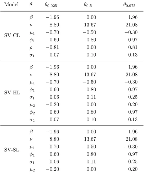
The priors on the evolution variances are inverted Gamma, with parameters of (2.5 , 0.025) forσ₁2and (11,0.1) forσ₂2. In the SV-CL model, we chose a Beta(2,2) prior on (ρ+ 1)/2, and an inverted Gamma for σ₁2 with parameters of (11,0.1). All the implied prior quantiles are given in Table 1.

Table 1_{. Prior quantiles}

Model θ θ₀.025 θ0.5 θ0.975 β −1.96 0.00 1.96 ν 8.80 13.67 21.08 SV-CL μ1 −0.70 −0.50 −0.30 φ1 0.60 0.80 0.97 ρ −0.81 0.00 0.81 σ1 0.07 0.10 0.13 β −1.96 0.00 1.96 ν 8.80 13.67 21.08 μ₁ −0.70 −0.50 −0.30 SV-HL φ1 0.60 0.80 0.97 σ₁ 0.06 0.11 0.25 μ₂ −0.20 0.00 0.20 φ2 0.60 0.80 0.97 σ₂ 0.07 0.10 0.13 β −1.96 0.00 1.96 ν 8.80 13.67 21.08 SV-SL μ1 −0.70 −0.50 −0.30 φ₁ 0.60 0.80 0.97 σ₁ 0.06 0.11 0.25 μ2 −0.20 0.00 0.20

SV-CL: conventional leverage; SV-HL: hierarchical leverage; SV-SL: simple leverage; θα: prior quantile at probabilityα.

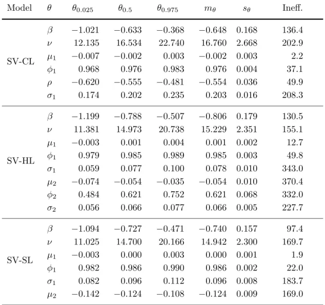
In Table 2, we report posterior replication summaries for the three models, based on 50000 replications obtained after discarding 5000 burn-in passes. In

Table 2. Posterior replication summaries (S&P500 data, GHSST stochastic volatility model, 1993 to 2014)

Model θ θ0.025 θ0.5 θ0.975 mθ sθ Ineff. β −1.021 −0.633 −0.368 −0.648 0.168 136.4 ν 12.135 16.534 22.740 16.760 2.668 202.9 SV-CL μ1 −0.007 −0.002 0.003 −0.002 0.003 2.2 φ₁ 0.968 0.976 0.983 0.976 0.004 37.1 ρ −0.620 −0.555 −0.481 −0.554 0.036 49.9 σ₁ 0.174 0.202 0.235 0.203 0.016 208.3 β −1.199 −0.788 −0.507 −0.806 0.179 130.5 ν 11.381 14.973 20.738 15.229 2.351 155.1 μ1 −0.003 0.001 0.004 0.001 0.002 12.7 SV-HL φ1 0.979 0.985 0.989 0.985 0.003 49.8 σ₁ 0.059 0.077 0.100 0.078 0.010 343.0 μ2 −0.074 −0.054 −0.035 −0.054 0.010 370.4 φ₂ 0.484 0.621 0.752 0.621 0.068 332.0 σ2 0.056 0.066 0.077 0.066 0.005 227.7 β −1.094 −0.727 −0.471 −0.740 0.157 97.4 ν 11.025 14.700 20.166 14.942 2.300 169.7 SV-SL μ1 −0.003 0.000 0.003 0.000 0.001 1.9 φ₁ 0.982 0.986 0.990 0.986 0.002 22.0 σ1 0.082 0.096 0.112 0.096 0.008 183.7 μ₂ −0.142 −0.124 −0.108 −0.124 0.009 169.0

SV-CL: conventional leverage; SV-HL: hierarchical leverage; SV-SL: simple leverage; θα: posterior quantile at probabilityα;

m_θ: posterior mean; s_θ: posterior standard deviation;

all cases, the posterior ordinate at β = 0 is negligible, confirming the skewness of the observation distribution since the prior mode of β is zero (see Dickey, 1971; Verdinelli and Wasserman, 1995). There is high persistence in the log-volatility process but it does not appear to be integrated. There is negligible posterior support forν <8, implying the existence of the first four moments of the observation distribution. As expected, all three models imply a very significant leverage effect: the posterior credible intervals for μ₂ and ρ only cover negative values, in spite of prior distributions that are symmetric about zero. In the SV-HL model, the autoregression coefficient of the leverage evolution equation (φ₂) is reasonably well identified, but its posterior is more diffuse than that of φ1. The inefficiency factors of the leverage evolution equation parameters are quite high; this suggests that the SV-HL model might be over-parameterized. Indeed, in this model, the largest posterior contemporaneous correlation occurs between μ₂ and φ₂, with a value of 0.92.

We now discuss model comparison. Marginal likelihoods were estimated for the three stochastic volatility models by the method of Section 4, using 2000 independent importance replications and 2000 posterior replications drawn with-out replacement from the MCMC sample; the filter of Section 4 usedN = 1000 particles. We also estimated the marginal likelihood for the GHt-GARCH model in Deschamps (2012), using the prior described in that article. The GHt-GARCH observation equation is the same as (2.3), but the variance equation is determin-istic:

h2_t =α∗₀+ [α∗₁I(yt−1 ≥0) +α2∗I(yt−1 <0)]yt2−1 +β∗h2t−1

where the α∗_i > 0, 0 < β∗ < 1, I is an indicator function, h2₀ = y2₀, and the likelihood is conditional on y₀.

Table 3 presents the natural logarithms of the marginal likelihoods, as well as the decimal logarithms of the Bayes factors against the GHt-GARCH model. Using the decimal logarithm enables model comparison using the Jeffreys scale (Jeffreys, 1961) where the evidence is treated as strong if log₁₀(BF) < −1 and decisive if log₁₀(BF) < −2. GHt-GARCH turns out to dominate all the other models. This conclusion is not entirely unexpected (Kim et al., 1998; Geweke and Amisano, 2010). However, ours appears to be the first formal comparison involving both asymmetric heavy-tailed errors and leverage for all models, since the two papers mentioned above compared a t-GARCH model with a Gaussian

Table 3_{. Marginal likelihoods and Bayes} factors (S&P500 data, 1993 to 2014)

Model log_ep(y) log₁₀(BF) NSE

GHt-GARCH −7236.83 0.00 0.00

SV-SL −7254.84 −7.82 0.01

SV-HL −7269.86 −14.35 0.01

SV-CL −7286.14 −21.42 0.02

p(y): marginal likelihood;

BF: Bayes factor against GHt-GARCH; NSE: numerical standard error of log₁₀(BF).

stochastic volatility model, and neither model allowed for the leverage effect. It is interesting that the conclusions of these authors turn out to be robust when extensions of both models are considered. Among the stochastic volatility formulations, simple leverage dominates hierarchical leverage, and both these models strongly dominate conventional leverage. This information is useful since adding a lagged endogenous variable to the state equation is a trivial extension of any stochastic volatility model, and might therefore facilitate the inclusion of leverage in other contexts.

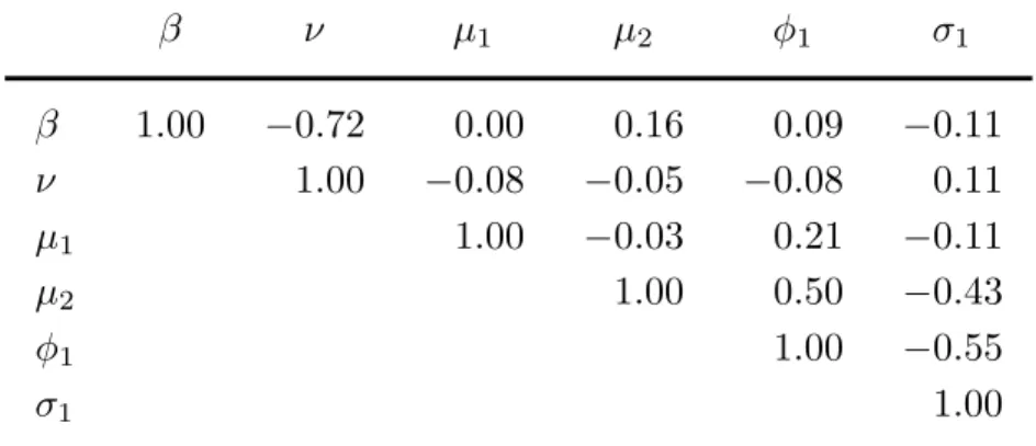
Table 4_{. Correlation matrix of posterior replications} (SV-SL model, S&P500 data, 1993 to 2014)

β ν μ₁ μ₂ φ₁ σ₁ β 1.00 −0.72 0.00 0.16 0.09 −0.11 ν 1.00 −0.08 −0.05 −0.08 0.11 μ1 1.00 −0.03 0.21 −0.11 μ2 1.00 0.50 −0.43 φ₁ 1.00 −0.55 σ1 1.00

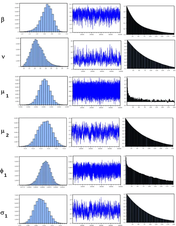
Table 4 reports the contemporaneous posterior correlations between the pa-rameters of the best stochastic volatility model (SV-SL). They suggest that the model is not over-parameterized. Figure 1 shows the posterior histograms, sam-ple paths, and correlograms for this model. These results are comparable to the ones obtained by Nakajima and Omori (2012) with a different parameteriza-tion of the generalized hyperbolic distribuparameteriza-tion and with the convenparameteriza-tional leverage formulation.

Figure 2 plots the observations, the posterior medians of the conditional stan-dard errorsht obtained with SV-SL, and the differences between these medians and the ones obtained under SV-CL and SV-HL. These differences are larger when SV-SL and SV-CL are compared, and suggest that SV-CL tends to under-estimate the volatility, especially during periods of instability.

However, the estimates are similar during periods of low volatility, so that the relative performance of the models might be different when the sample period is restricted to the most recent years (including the recent financial crisis). This can be assessed by splitting the sample into two subsamples yA and yB of ap-proximately equal sizes and estimating marginal likelihoods for each subsample. The predictive marginal likelihood for the most recent years (see Geweke, 2005, p. 66) is defined as: p(yB |yA) = p(y_p(yA,yB) A) = p(yB|yA,θ)p(yA |θ)p(θ)dθ p(yA |θ)p(θ)dθ = p(yB |yA,θ)p(θ |yA)dθ

showing that the subjective prior p(θ) is replaced by the posterior p(θ | yA), which is presumably less sensitive thanp(θ) to prior judgments. This is especially important when nonnested models such as GARCH and SV are considered, since their priors are difficult to compare.

We report in Table 5 the predictive marginal likelihoods and Bayes factors for the period ranging from January 6, 2004 to August 11, 2014, conditional on the training sample ranging from January 6, 1993 to January 5, 2004. For comparison, their unconditional counterparts are also given. The Bayes factor evidence in favor of the SV-SL model against SV-HL becomes weaker in Table 5 than in Table 3: it is strong rather than decisive according to the unconditional Bayes factor, and becomes very weak according to the predictive one. This

confirms the intuition provided by Figure 2. However, the model ordering remains the same. This suggests that our conclusions on model comparison are robust, since predictive Bayes factors are relatively insensitive to the prior.

Table 5_{. Marginal likelihoods and Bayes} factors (S&P500 data, 2004 to 2014)

Unconditional Predictive

Model log_ep(yB) log10(BF) NSE logep(yB |yA) log10(BF) NSE

GHt-GARCH −3517.11 0.00 0.00 −3505.47 0.00 0.00

SV-SL −3546.07 −12.58 0.02 −3520.43 −6.50 0.02

SV-HL −3549.32 −13.99 0.02 −3521.15 −6.81 0.02

SV-CL −3564.04 −20.38 0.02 −3535.45 −13.02 0.02

p(•): marginal likelihood; y_A: observations for 1993-2003;

yB: observations for 2004-2014; BF: Bayes factor against GHt-GARCH; NSE: numerical standard error of log₁₀(BF).

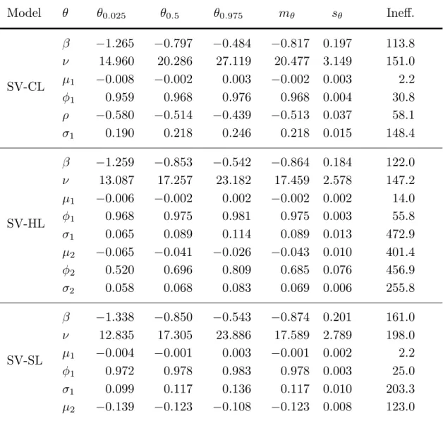
5.2 SMI data. Our second sample consists of the Swiss Market Index (SMI) daily log-returns for the period ranging from January 4, 1993 to December 29, 2014 (5683 observations). The same prior as in Section 5.1 was used. Table 6 presents posterior replication summaries for the three stochastic volatility models; the results are very similar to those obtained with the S&P500 data, suggesting that they are representative of the time period involved. Table 7 presents the Bayes factors against the GHt-GARCH model based on the full sample, as well as the conditional Bayes factors obtained by using the observations ranging from January 4, 1993 to December 31, 1996 as a training sample.

Table 7 shows that the ranking between the three stochastic volatility models is the same for the SMI data as for the S&P500 data: SV-SL dominates SV-HL, and both SV-SL and SV-HL dominate SV-CL. However, the ranking between GHt-GARCH and SV-SL differs from the one obtained in Tables 3 and 5 with the S&P500 data. When the entire sample is considered, the Bayes factor evidence in favor of GHt-GARCH is strong rather than decisive; and for the last 18 years

Table 6. Posterior replication summaries (SMI data, GHSST stochastic volatility model, 1993 to 2014)

Model θ θ0.025 θ0.5 θ0.975 mθ sθ Ineff. β −1.265 −0.797 −0.484 −0.817 0.197 113.8 ν 14.960 20.286 27.119 20.477 3.149 151.0 SV-CL μ1 −0.008 −0.002 0.003 −0.002 0.003 2.2 φ₁ 0.959 0.968 0.976 0.968 0.004 30.8 ρ −0.580 −0.514 −0.439 −0.513 0.037 58.1 σ₁ 0.190 0.218 0.246 0.218 0.015 148.4 β −1.259 −0.853 −0.542 −0.864 0.184 122.0 ν 13.087 17.257 23.182 17.459 2.578 147.2 μ1 −0.006 −0.002 0.002 −0.002 0.002 14.0 SV-HL φ1 0.968 0.975 0.981 0.975 0.003 55.8 σ₁ 0.065 0.089 0.114 0.089 0.013 472.9 μ2 −0.065 −0.041 −0.026 −0.043 0.010 401.4 φ₂ 0.520 0.696 0.809 0.685 0.076 456.9 σ2 0.058 0.068 0.083 0.069 0.006 255.8 β −1.338 −0.850 −0.543 −0.874 0.201 161.0 ν 12.835 17.305 23.886 17.589 2.789 198.0 SV-SL μ1 −0.004 −0.001 0.003 −0.001 0.002 2.2 φ₁ 0.972 0.978 0.983 0.978 0.003 25.0 σ1 0.099 0.117 0.136 0.117 0.010 203.3 μ₂ −0.139 −0.123 −0.108 −0.123 0.008 123.0

SV-CL: conventional leverage; SV-HL: hierarchical leverage; SV-SL: simple leverage; θα: posterior quantile at probabilityα;

m_θ: posterior mean; s_θ: posterior standard deviation;

Table 7_{. Marginal likelihoods and Bayes factors (SMI data)}

Unconditional 1993-2014 Predictive 1997-2014 Model log_ep(y) log₁₀(BF) NSE log_ep(yB |yA) log10(BF) NSE

GHt-GARCH −7715.17 0.00 0.00 −6512.32 0.00 0.00

SV-SL −7717.87 −1.17 0.01 −6507.36 2.15 0.02

SV-HL −7729.31 −6.14 0.01 −6520.36 −3.49 0.02

SV-CL −7749.34 −14.84 0.02 −6528.38 −6.97 0.02

p(•): marginal likelihood; yA: observations for 1993-1996;

yB: observations for 1997-2014; BF: Bayes factor against GHt-GARCH; NSE: numerical standard error of log₁₀(BF).

of the sample (1997 to 2014) the predictive Bayes factor decisively favors SV-SL over GHt-GARCH.

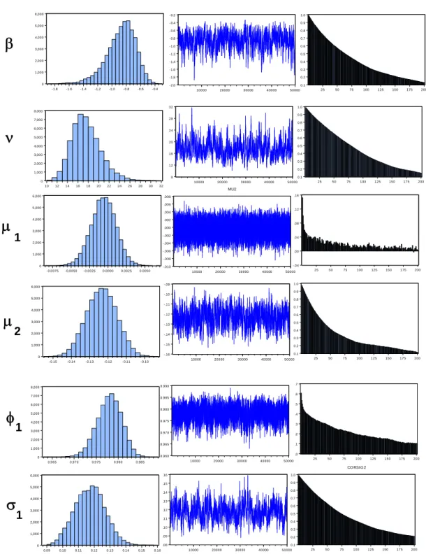
Finally, Figure 3 presents the histograms, sample paths and correlograms for the best SV model; they are very similar to those in Figure 1. Figure 4 presents the posterior medians of the square root volatilities ht in this model, and the differences these medians and the ones obtained under the other leverage formu-lations. Figure 4 is very similar to Figure 2; in particular, the volatility estimates under SV-SL tend to dominate those under SV-CL, and the differences are more apparent during periods of high volatility.

6. Conclusions

This paper has compared three different formulations of the leverage effect in a stochastic volatility model with a skewed and heavy-tailed observation distri-bution. Including the past log-return as a covariate in the evolution equation dominates the conventional formulation where the observation and evolution er-rors are correlated. Furthermore, the coefficient of this covariate appears to be constant over time. This appears to be a characteristic of smoothed, rather than predicted, log-volatilities, since the predicted volatilities in the EGARCH model of Nelson (1991) are known to generally imply an asymmetric news impact func-tion.

Knowing that a simple formulation of leverage can be superior to the conven-tional one is useful for the following reason. Imposing the convenconven-tional leverage formulation is not practical when the observation distribution is not condition-ally Gaussian, since this formulation uses the properties of the Gaussian distri-bution. By contrast, the simple addition of a lagged endogenous variable should be straightforward in any stochastic volatility model.

The stochastic volatility model was also compared with a threshold GARCH formulation having the same observation distribution. To the best of the author’s knowledge, this is the first comparison involving both skewed and heavy-tailed errors in both models. The stochastic volatility model turned out to yield a significantly higher marginal likelihood with Swiss Market Index data ranging from 1997 to 2014. However, GARCH was superior to SV in all the other samples. Finally, this paper has documented the good performance of an algorithm that combines existing particle smoothing methods with a block sampler of the type proposed by Shephard and Pitt (1997). In the author’s view, this technique offers several advantages over existing ones. First, since it inherits the flexibility and generality of particle methods, it can be applied to observation densities that are not log-concave and to evolution equations that are nonlinear. Second, its analytical requirements are more modest than those of methods based on Laplace approximations to the observation density. Third, its effectiveness only requires a relatively small number of particles that does not depend on the sample size, contrary to the particle MH method proposed by Andrieu et al. (2010). Last, the method is effective with simple particle filters: the computational cost of the filter of Section A.7 is linear in the numberN of particles, whereas that of the auxiliary filter advocated by Pitt et al. (2012) for particle MH methods is a quadratic function of N. The use of our method in other contexts therefore appears to be an interesting topic for further research.

Appendix A. A complete description of the posterior simulator

In Sections (A.1) to (A.7), we will describe our posterior simulator for the model with GHSST errors and time-varying leverage effects; the minor modifica-tions that must be made to that algorithm when the model is the conventional one, where the volatility equation is based on (2.6) with E(₀t1,t+1) = ρ, will be described in Section A.8. Finally, Section A.9 will give some details on the

performance of the method. A.1 Simulating μ.

We reformulate (2.7)–(2.10) as:

z_i =X_iμ_i+σ_ii, (i= 1,2) (A.1)

wherei = (i0i1. . . iT) and where:

z_i = ⎛ ⎜ ⎜ ⎜ ⎜ ⎝ 1−φ2 i λi0 ˜ λ_i1−φ_iλ_i0 .. . ˜ λiT −φiλi,T−1 ⎞ ⎟ ⎟ ⎟ ⎟ ⎠ (A.2) Xi= ⎛ ⎜ ⎜ ⎜ ⎜ ⎝ √ 1−φ2 i 1−φi 1 .. . 1 ⎞ ⎟ ⎟ ⎟ ⎟ ⎠ (A.3)

with ˜λ2t =λ2t and ˜λ1t =λ1t−λ2tyt−1. Using the conditionally conjugate prior μi ∼ N(μ_i, θ2i), the full conditional posterior of μi is the Normal distribution N(μ_i,Θ2_i) with: Θ2_i = X_iX_i σ2 i + 1 θ2 i −1 μ_i = Θ2_i X_izi σ2 i + μi θ2 i . A.2 Simulating φ. We reformulate (2.8)-(2.9) as:

wi=Wiφi+σi∗_i (i= 1,2) (A.4) where∗_i = (i1. . . iT), and: wi = ⎛ ⎜ ⎝ ˜ λi1−μi .. . ˜ λiT −μi ⎞ ⎟ ⎠, Wi = ⎛ ⎝ λ_i0 .. . λi,T−1 ⎞ ⎠.

We use as prior on φi the truncated Normal distribution T N(φ_i, ψi2), with support −1 < φi < 1. Since φi enters nonlinearly in the distribution of λi0,

draws require a Metropolis-Hastings (MH) step. We draw a candidate φi from the truncated NormalT N(φ_i,Ψ2_i), where:

Ψ2_i = W_iWi σ2 i + 1 ψ2 i −1 φ_i = Ψ2_i W_iwi σ2 i + φi ψ2 i and accept the candidate with probability:

min 1, g(φi) g(φold i ) where: g(φi) = 1−φ2 i exp ⎡ ⎢ ⎣− λi0 − ₁₋μi_φi 2 (1−φ2 i) 2σ2 i ⎤ ⎥ ⎦

and φold_i is the previous draw. If the candidate is rejected, φold_i is retained. For a justification of this rejection rule, see Chib and Greenberg (1995, Section 5). A.3 Simulating σ.

We use as prior on σ2

i an inverted Gamma distribution with parameters ai and bi. Equation (A.1) implies vi =σii, with vi = zi −Xiμi and where the zi and Xi are defined in (A.2) and (A.3). The conditional posterior of σ2i is then an inverted Gamma with parameters:

a∗_i =ai+ T + 1 2 and b ∗ i =bi+ v ivi 2 . A.4 Simulating Z.

As noted by Barndorff-Nielsen (1997), the full conditional posterior of Zt is Generalized Inverse Gaussian (see Jørgensen, 1982):

p(Zt |λ1t, yt, ν, β)∝ Z− (ν+3) 2 t exp −1 2 χtZt−1 +β2Zt where: χt = ytexp −λ1t 2 + δ2β ν−2 2 +δ2

and δ2 _{is given by (2.2). An efficient algorithm for drawing Zt from this} distri-bution is described in Deschamps (2012).

A.5 Simulating β and ν.

This step relies on tailored MH proposals (see Chib and Greenberg, 1994, 1995) and is a minor adaptation of the method used in Deschamps (2012). The conditional posterior log-kernel can be written as:

k(ν, β) = lnp(ν, β) + T $ t=0 kt(ν, β), with: kt(ν, β) =− ytexp(−λ1t/2)−β % Zt− _νδ₋₂2 &2 2Zt + ν 2ln δ2 2 −ln Γν 2 −ν 2 + 1 lnZ_t− δ2 2Zt where p(β, ν) is a prior log-kernel with support {(ν, β) | ν > 4,−∞< β < ∞}, andδ2 is given by (2.2) as a function of β andν. We defineξ= (ξ1, ξ2) = [ln(ν− 4), β], and ˜kt(ξ) =kt[exp(ξ1) + 4, β]. Let (ν∗, β∗) be an approximate maximizer

of k(ν, β) under the constraint ν > 4. A vector ξ is drawn from a bivariate

Student distribution with 3 degrees of freedom, expectation ξ∗ = [ln(ν∗−4), β∗] and scale matrix:

Σ = ⎡ ⎣$T t=0 ∂˜k_t ∂ξ ∂˜k_t ∂ξ ξ∗ ⎤ ⎦ −1 .

The candidate (ν, β) = (exp(ξ1) + 4, ξ2) is accepted with probability:

min

1,exp %

k(ν, β)−k(νold, βold)+

lnfST[ln(νold−4), βold]−ln(νold −4)−lnfST[ln(ν−4), β] + ln(ν −4) &

wherefST[•] denotes the bivariate Student proposal density. If (ν, β) is rejected, (νold, βold) is retained.

A.6 Simulating λ2.

Equations (2.8)–(2.10) may be written as:

λ2t =μ2+φ2λ2,t−1+σ22t for t = 1, . . . , T λ₂₀ ∼N μ₂ 1−φ2 , σ22 1−φ2 2 with: z_t∗ = λ1t −μ1−φ1λ1,t−1.

This is a linear Gaussian state space model conditional on y and λ1, so that the full conditional posterior ofλ2 can be simulated by forward filtering backward sampling (FFBS). In the forward recursion, we use the Kalman filter (see, e.g, Harvey, 1989, pp. 105-106) to construct the Gaussian filter densities:

Ft(λ2t |λ10, . . . , λ1t)

yielding in particular the full conditional posteriorF_T(λ_2T |λ1) from which λ_2T is sampled. In the backward recursion, we then successively sample λ_2,t−1 for t=T, T −1, . . . ,1, from the densities:

F_t∗₋₁(λ2,t−1 |λ1, λ2t)∝

Ft−1(λ2,t−1 |λ10, . . . , λ1,t−1)fN(λ2t;μ2+φ2λ2,t−1, σ22) (A.5) where fN is the Normal density; they are straightforward Bayesian updates of the filter densities of λ₂,t−1. For a justification, see Carter and Kohn (1994) or Kim and Nelson (1999).

Drawing from (A.5) simply implies simulating (λ₂,T−1, . . . , λ20) from a back-ward Gaussian autoregression, with parameters that can be obtained from the Kalman filter recursion and from the expressions given by Kim and Nelson (1999, p. 193).

A.7 Simulating λ1.

The relevant observation density can be written as:

pt(yt |λ1t) =fN(yt;θtexp(λ1t/2), Ztexp(λ1t)) (A.6) withθt =β(Zt−δ2/(ν−2)) and for t = 0, . . . , T. The evolution density is:

pt+1(λ1,t+1 |λ1t) =fN(λ1,t+1;μ1+φ1λ1t+λ2,t+1yt, σ21) for t= 0, . . . , T −1 (A.7)

p0(λ10) =fN λ10; μ1 1−φ1, σ2₁ 1−φ2 1 . (A.8)

Since this is a nonlinear state space model, the method of Section A.6 is no longer applicable, and the MH algorithm is appropriate. In order to draw MH candidates, we propose to replace the recursion (A.5) by a backward autoregres-sion with parameters estimated by least squares from a few replications of the particle smoother of Godsill et al. (2004). We first run a suitable particle filter to obtainN(T + 1) drawsλi_1t with associated normalized importance weightsπi_t, for t = 0, . . . , T and i = 1, . . . , N. We then draw a path λ₁∗ = (λ∗_1t)T_t=0 from an approximate smoothing distribution by the following method:

(1) Draw λ∗_1T from the filter sample λ1

1T, . . . , λN1T using the probability dis-tribution (π1

T, . . . , πNT );

(2) For t = T − 1, . . . ,0, successively draw λ∗_1t from the filter sample λ1_1t, . . . , λN_1t using probabilities proportional to:

π1_t pt+1(λ∗1,t+1 |λ11t), . . . , πtNpt+1(λ∗1,t+1 |λN1t).

Once several pathsλj₁, forj = 1, . . . , M, have been drawn by this method, it is a simple matter to find least squares estimates of the parameters of the following backward autoregression:

λj_1T =aT +V_T1/2η_Tj (A.9)

λj_1,t−1 =at−1+ Φt−1λ1jt+Vt1−1/2ηtj−1 (A.10) withη_Tj andη_tj₋₁ ∼Niid(0,1) for t= 1, . . . , T andj = 1, . . . , M.

Unfortunately, MH candidates generated from estimates of (A.9)–(A.10) will typically suffer from high rejection rates when T is large. This phenomenon, which has also been noted by Shephard and Pitt (1997) with linear Gaussian proposal models based on Laplace approximations, is similar to the degeneracy problem in the particle filtering literature: for largeT, the errors in approximat-ing the complete data density of the true model will accumulate so that most importance weights will become zero. Following Shephard and Pitt (1997), we will therefore divide the full state vectorλ1 into complementary blocks with ran-dom endpoints for implementing the MH algorithm of this section, and will use the rejection method advocated by Tierney (1994, p. 1707) for proposing MH candidates. A description of this algorithm follows.

(1) Choose a tuning parameterK ≥1 defining the numberK+ 1 of random blocks.

(2) Compute the knots k0 =−1,kK+1 =T, andki = int[T(i+Ui)/(K + 2)] for i= 1, . . . , K, whereUi∼ U(0,1) and int[•] denotes the integer part. (3) For i = 0, . . . , K, define λi₁ as the subvector of λ1 containing all λ1t for

ki+ 1≤t≤ki+1.

(4) Draw λi₁, conditional on the remaining blocks, from (A.9)–(A.10) with aT, VT, at−1, Φt−1, and Vt−1 replaced by their least squares estimates from the particle smoother output. Letfi(λi₁) be the conditional density of the drawn value, and let:

m_i(λi₁) = ⎡ ⎣ ki+1 t=ki+1 p_t(y_t |λ_1t)p_t(λ_1,t|λ_1,t−1) ⎤

⎦p_ki+1+1(λ_1,ki+1+1 |λ_1,ki+1) where we use the conventions that p_T+1(λ_1,T+1 | λ_1T) = 1 and p₀(λ₁₀ | λ_1,−1) =p₀(λ₁₀). Accept λi₁ with probability:

min 1, mi(λ i 1) cifi(λi₁)

whereciis a pseudo-dominating constant that can be chosen as a high em-pirical quantile ofmi(λi₁)/fi(λi₁), obtained from a few replications. Using 100 replications and the 99th percentile of this ratio yields a reasonable compromise between computational cost and acceptance probabilities. If λi

1 is rejected go to (4).

(5) The density of the accepted candidate in step (4) is proportional to: qi(λi1) = min[mi(λ1i), cifi(λi1)].

In the MH rejection step, we accept this draw with probability:

min 1, mi(λ i 1) mi(λi,₁old) qi(λi,₁old) qi(λi₁)

where λi,₁old is the previous draw. If the candidate is rejected λi,₁old is retained.

We conclude this section by describing a partially adapted (in the sense of Pitt and Shephard, 1999) particle filter for λ1. Equation (A.6) may be viewed as a

likelihood of λ1t; this likelihood is not globally log-concave when θt = 0 but has a unique maximum that can be found analytically. Indeed, its first derivative is:

∂lnpt(yt |λ1t) ∂λ₁t = 1 2Zt[exp(−λ1t)y 2 t −ytθtexp(−λ1t/2)−Zt]. (A.11) Equating (A.11) to zero yields the following roots:

exp(−λ₁t/2) = θt±

θ2 t + 4Zt 2yt and the admissible solution:

¯ λ1t =−2 ln θt+θ2t + 4Zt 2yt if yt > 0 =−2 ln θt− θ2 t + 4Zt 2yt if yt < 0. (A.12)

The second derivative is: ∂2_{lnpt(yt |λ} 1t) ∂λ2 1t = 1 4Zt[−2 exp(−λ1t)y 2 t +ytθtexp(−λ1t/2)]. (A.13) Inserting (A.12) into (A.13) yields:

∂2lnpt(yt |λ1t) ∂λ2 1t _¯ λ1t = −2 + 2θt θ2 t + 4Zt −1 ifyt >0 = −2− 2θt θ2 t + 4Zt −1 ify_t <0 (A.14) and it can be checked that (A.14) is always negative.

The preceding discussion suggests using, as an importance density for a parti-cle filter, the following posterior approximation based on a Taylor series expansion of lnpt(yt |λ1t) around ¯λ1t: pt(λ1t |yt, λ1,t−1)≈fN(λ1t;m∗t(λ1,t−1), v1∗t) (A.15) with: 1 v₁∗_t = 1 σ₁2_t + 1 2 1−sign(y_t)√ θt θ2 t+4Zt (A.16)

m∗_t(λ_1,t−1) =v∗_1t ⎛ ⎜ ⎜ ⎝mt(λ_σ12,t−1) 1t + λ¯1t 2 1−sign(yt)√_θ2θt t+4Zt ⎞ ⎟ ⎟ ⎠ (A.17) and where: m0(λ1,−1) = μ1 1−φ₁, σ 2 10 = σ₁2 1−φ2 1 , m_t(λ_1,t−1) =μ₁ +φ₁λ_1,t−1+λ_2,ty_t−1, and σ₁2_t =σ₁2 for t = 1, . . . , T. In the (rare) cases where yt = 0, the likelihood has no finite maximum. We then base the particle filter importance density on the evolution equation only, and set ¯λ1t = 0 and v1∗t = σ12t in Equations (A.16)–(A.17); this is known as the “bootstrap filter” in the particle filtering literature.

It is now a simple matter to devise an appropriate particle filter for λ1. For t = 0, . . . , T, we draw N independent particles λi_1t (i = 1, . . . , N) from (A.15) with λ_1,t−1 = λi_1,t−1. Particle i is associated with the following importance weight: π_ti ∝ pt(yt |λ i 1t)pt(λi1t |λi1,t−1) fN(λi₁t;m∗t(λi1,t−1), v1∗t) ×π_ti₋₁

whereπi₋₁ ≡1/N, and p₀(λ₁₀ |λ₁,−1) =p0(λ10). If the effective sample size: EFFNt = _N 1

i=1(πti)2

is less than 0.5N (say), resampling is performed (see Kitagawa, 1996, or Maskell, 2004, p. 57).

A.8 Estimating the conventional leverage model.

In this section, we describe the modifications that must be made to the pos-terior simulator when the volatility evolution equation is based on (2.6) rather than (2.8), withE(0t1,t+1) =ρ. For ease of notation, since (2.9) and (2.10) are no longer part of the model, we set λ1,t+1 = λt+1, and (μ1, φ1, σ1) = (μ, φ, σ). Replacing σ11,t+1 in Equation (2.6) by its conditional counterpart yields, for t= 0, . . . , T −1: λt+1 =μ+φλt+ρσ0t + σ2₍₁−_ρ2_)ηt+1 =μ+φλt+ √ρσ Zt ytexp −λt 2 −β Zt − δ 2 ν−2 + σ2₍₁−_ρ2_)ηt+1 (A.18)

and the definitions ofpt+1(λ1,t+1 |λ1t), mt(λ1,t−1), andσ12t in (A.7) and (A.17) must be modified accordingly; these are the only changes in the algorithm of Section A.7. The simulation of μ and φ conditional on λ, ρ, σ, β, ν,Z,y is done as in Sections A.1 and A.2, upon replacing ˜λ1t by:

λ∗_t =λt− ρσ Zt−1 yt−1exp −λt−1 2 −β Zt−1− δ 2 ν−2 (A.19)

and dividingw₁, W₁, and the lastT elements of z₁ and X₁ by 1−ρ2_.

Conditional on (μ, φ,λ, β, ν,Z,y), ρ and σ are simulated in one block, using tailored MH proposals as in Section A.5; a similar method was used by Nakajima and Omori (2012). The conditional posterior log-kernel is:

h(ρ, σ) = lnπ(ρ, σ) + T $ t=1 ht(ρ, σ)− λ0− ₁₋μ_φ 2 (1−φ2) 2σ2 −lnσ

whereπ(ρ, σ) is a prior kernel with support{(ρ, σ)| |ρ|<1, σ >0} and: ht(ρ, σ) =−1 2ln[σ 2_(1−ρ2_)]− 1 2σ2_(1−ρ2₎(λ ∗ t −μ−φλt−1)2 withλ∗_t given by (A.19) as a function of ρ and σ.

We define: ω= (ω₁, ω₂) = ln 1 +ρ 1−ρ ,lnσ ˜ ht(ω) =ht exp(ω₁)−1 exp(ω₁) + 1,exp(ω2)

and let (ρ∗, σ∗) be an approximate maximizer of h(ρ, σ) under the constraints |ρ|<1, σ >0. A vector ω is drawn from a bivariate Student distribution with 3 degrees of freedom, with expectation:

ω∗ = ln 1 +ρ∗ 1−ρ∗ ,lnσ∗ and with scale matrix:

Σ∗ = _T $ t=1 ∂˜ht ∂ω ∂˜ht ∂ω ω∗ −1 .

The candidate:

(ρ, σ) =

exp(ω₁)−1

exp(ω1) + 1,exp(ω2) is accepted with probability:

min

1,exp %

h(ρ, σ)−h(ρold, σold) + lnfST[ω1old, ωold2 ]−ln(σold)

−ln(1−ρ2 old)−lnfST(ω1, ω2) + ln(1−ρ2) + ln(σ) & where fST[•] denotes the bivariate Student proposal density, (ρold, σold) is the previous draw, and:

(ω₁old, ω₂old) = ln 1 +ρold 1−ρold ,lnσold . If (ρ, σ) is rejected, (ρold, σold) is retained.

A.9 Algorithm performance.

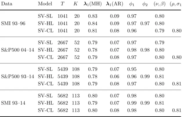
To conclude this Appendix, we comment briefly on the performance of the MCMC algorithm described in Section A.7 and used for simulating λ1. Im-plementing this algorithm requires the choice of three tuning parameters: the numberN of filter particles; the number M of particle smoother paths; and the numberK + 1 of blocks in λ1. For all the simulations described in Sections 5.1 and 5.2, involving three different leverage formulations and five different sample sizes, the same tuning parameter values of N = 2000 and M = 100 were used. The number of blocks was chosen as the integer nearest toT /B, with B= 10 for the first 100 MCMC sweeps andB = 50 otherwise. The average MH acceptance probability crucially depends onB, which is an approximate expected block size. Table 8 shows the average acceptance probabilities (after burn-in) for the three stochastic volatility models and for four different sample sizes. They are remark-ably similar across models and sample sizes, in spite of the fact that the same values ofN,M, andBwere used throughout the simulations. This suggests that the method of Section A.7 is generally applicable beyond the models estimated in this paper.

Appendix B. A description of the particle filter used for marginal likelihood estimation