University of Massachusetts Amherst
ScholarWorks@UMass Amherst
Masters Theses 1911 - February 2014
2013
Comparison And Application Of Methods To
Address Confounding By Indication In
Non-Randomized Clinical Studies
Christine Marie Foley
University of Massachusetts AmherstFollow this and additional works at:
https://scholarworks.umass.edu/theses
This thesis is brought to you for free and open access by ScholarWorks@UMass Amherst. It has been accepted for inclusion in Masters Theses 1911 -February 2014 by an authorized administrator of ScholarWorks@UMass Amherst. For more information, please contact
Foley, Christine Marie, "Comparison And Application Of Methods To Address Confounding By Indication In Non-Randomized Clinical Studies" (2013).Masters Theses 1911 - February 2014. 1121.
Comparison and Application of Methods to Address Confounding by Indication in Non-Randomized Clinical Studies
A Thesis Presented by
CHRISTINE M FOLEY
Submitted to the Graduate School of the
University of Massachusetts Amherst in partial fulfillment of the requirements for the degree of
MASTER OF SCIENCE September 2013
Biostatistics
Keywords: Antidepressant medication, type 2 diabetes, epidemiology, marginal structural models, propensity score, survival analysis
Comparison and Application of Methods to Address Confounding by Indication in Non-Randomized Clinical Studies
A Thesis Presented By
CHRISTINE M. FOLEY
Approved as to style and content by:
_________________________________________________ Raji Balasubramanian, Chair
_________________________________________________ Penelope Pekow, Member
_________________________________________________ Yunsheng Ma, Member
_________________________________________________ Brian Whitcomb, Member
_____________________________________________ Paula Stamps, Graduate Program Director Department of Public Health
iii
ABSTRACT
COMPARISON AND APPLICATION OF METHODS TO ADDRESS CONFOUNDING BY INDICATION IN NON-RANDOMIZED CLINICAL STUDIES
SEPTEMBER 2013
CHRISTINE M FOLEY, B.S., WORCESTER STATE UNIVERSITY M.S., UNIVERSITY OF MASSACHUSETTS AMHERST
Directed by: Professor Raji Balasubramanian
Objective: The aim of this project was to apply and compare marginal structural models, and propensity score adjusted models with traditional Cox Proportional Hazards models to address confounding by indication due to the presence of time-dependent confounders. These methods were applied to data from approximately 120,000 women enrolled in the Women’s Health Initiative (WHI) to evaluate the causal effect of antidepressant medication use with respect to type 2 diabetes risk.
Methods: Four approaches were compared. Three traditional Cox Models were used. The first used only baseline covariates. The second used time-varying antidepressant medication use, BMI and presence of elevated depressive symptoms and adjusted for all other covariates measured at baseline. The third used time-varying antidepressant medication use, BMI and presence of elevated depressive symptoms and adjusted for other baseline covariates, with additional adjustment for propensity to taking antidepressants at baseline. Our fourth method used a Marginal Structural Cox Model with Inverse Probability of Treatment Weighting that included time-varying antidepressant medication use, BMI and presence of elevated depressive symptoms and adjusted for all other covariates measured at baseline.
iv
Results: All approaches showed an increase in diabetes risk for those taking antidepressant medication. The Cox Proportional Hazards models using only baseline covariates showed the lowest increase in risk (OR=1.21, 95% CI 1.07 - 1.36; OR=1.16, 95% CI 1.02 - 1.32, respectively). Diabetes risk increased with adjustment for time-dependent confounding and results for these three approaches were almost identical. All models were statistically significant. Ninety-five percent confidence intervals overlapped for all 4 approaches showing they were not significantly different from one another.
Conclusions: Our analyses did not find a difference in estimates between traditional Cox
Proportional Hazards Models and Marginal Structural Cox Models in the WHI cohorts. Estimates of the Inverse Probability of Treatment Weights were all very close to 1 which explains why we observed similar results with all four approaches.
Keywords: Antidepressant medication, type 2 diabetes, epidemiology, marginal structural models, propensity score, survival analysis
v TABLE OF CONTENTS Page ABSTRACT……….…iii LIST OF TABLES………..………..vii LIST OF FIGURES……….……..……….viii CHAPTER I. INTRODUCTION……….…………1 II. METHODS……….………….4
The Women’s Health Initiative (WHI)……….………..4
Outcome Ascertainment……….………..4
Time-Varying Exposure………..………….…...5
Time-Varying Confounders……….………….…...5
Other Confounders……….…….…………6
III. STATISTICAL ANALYSIS……….…………..7
Analysis Datasets……….….…….7
Approach 1 – Cox Proportional Hazards Model……….…….8
Approach 2 – Extended Cox Proportional Hazards Model……….….8
Approach 3 – Extended Cox Proportional Hazards Model Adjusting for Propensity……….…...……….8
vi
Page
IV. RESULTS……….12
V. DISCUSSION………15
APPENDIX - SAS CODE TO FIT THE MARGINAL STRUCTURAL COX PROPORTIONAL HAZARDS MODEL……….……….28 REFERENCES……….………33
vii
LIST OF TABLES
Table Page
1. Summary of Baseline Characteristics of the Study Sample…………..………17 2. Hazard Ratios Comparing Cox Proportional Hazards Models to Marginal
Structural Models………20 3. Inverse Probability of Treatment-Weighted Estimates Of The Parameters Of
A Marginal Structural Model For The Causal Effect Of Antidepressant Medication Use On Diabetes Risk………..…..………21 4. EstimatedProbability of Having One’s Own Observed Treatment History
And Censoring History At Follow- ……….………24 5. Estimate of Variation in Primary Exposure and Time-Dependent Confounder Variables (WHI-OS).……….……….…………..………25
viii
LIST OF FIGURES
Figure Page
1. Illustration of time-dependent confounding by BMI in the association of
antidepressant medication use and time to development of diabetes………26 2. Flow chart describing analytic cohort included for the investigation……….27
1
CHAPTER I INTRODUCTION
Diabetes is a chronic illness with serious health consequences, such as adult blindness, non-traumatic limb amputation, renal failure and neuropathy. Previous literature has noted considerable diabetes and depression among postmenopausal women, with a prevalence rate that is approximately 12% for each. 1, 2 As many as 25% of individuals live with both conditions. 3 Two separate meta-analyses demonstrated that adults with depression had a 37-60% increased risk of developing diabetes. 4, 5 The 2009 sub-analysis of the Melbourne Longitudinal Studies on Healthy Ageing (MELSHA) found that symptomatic depression predicts a 2-fold increase in diabetes incidence, with or without antidepressant use. 6
Recent literature suggests an increased risk of diabetes among those who are depressed and on antidepressant medications. 7-10 It is increasingly important to further investigate
whether depression or the antidepressant medication is influencing this association given that approximately 11% of American women take antidepressant medication, and use is rising. 11 While the rates of use for depression treatment has remained the same, off-label use of antidepressants has increased significantly. 12 Examples of antidepressant off-label use include treatment for certain type of pain, fibromyalgia, insomnia, and general unhappiness.
The Women’s Health Initiative (WHI) database is a valuable resource that can inform the association between antidepressant medication use/depression and diabetes risk in a population of post-menopausal women. It is a longitudinal study with a large sample size containing repeated measurements for presence of elevated depressive symptoms, self-reported diagnosis of type 2 diabetes and antidepressant medication use.
2
Ma and colleagues 13 found that elevated depressive symptoms and antidepressant medication use were significantly related to type 2 diabetes risk in both unadjusted and multivariable Cox models in the WHI. However, the WHI is a non-randomized setting in which there is the potential for several time-dependent confounders such as BMI to influence the causal relationship between antidepressant use and diabetes risk (Figure 1). In other words, participants with increased BMI or depression could be more likely to be on antidepressants in the future. Moreover, BMI and depression can also significantly influence future diabetes risk. Thus, a naïve analysis to evaluate the causal relationship between antidepressant use and diabetes risk could result in biased estimates of the effects of antidepressant medication use by misattributing the effects of time-dependent confounders such as BMI to treatment.
When research interest lies in the causal effect of a time varying exposure on outcome, in the presence of time-modified confounding, traditional Cox models can result in biased estimates that do not necessarily have causal interpretation (Figure 1). 14-16 In an observational study, it is difficult to guarantee balance of important potential confounding variables such as age, race/ethnicity, and gender between groups because participants were not randomized to either antidepressant medication users or non-users. If more participants in one level of the confounding variable are on treatment because of the influence of a time-dependent
confounder, we could falsely see a treatment effect when there is not one. A solution to this problem is the use of marginal structural models. Marginal structural models are appropriate when you have time-dependent confounding with a time-varying exposure. They aim to break the association between the exposure and confounder and provide balance between treatment and control across levels of the confounding variable. These methods can also be applied if your time-dependent confounder is influenced by prior treatment and is thus an intermediate.
3
The objective of this work was to apply and compare results obtained from standard approaches, such as multivariable Cox models and propensity score adjusted Cox models to those obtained from the application of IPTW marginal structural model methods developed for causal inference applicable to non-randomized settings. These methods were applied to data from approximately 68,000 women enrolled in the WHI-OS and approximately 52,000 women enrolled in the WHI-CT to evaluate the causal effect of antidepressant medication use with respect to type 2 diabetes risk.
The paper is organized as follows: In the Methods section, we describe our study population, timing of our measurements, instruments used and our modeling approaches. We also describe our outcome measures, along with time varying exposures and confounders considered. In the Results section, we present results obtained by applying the four approaches we used to estimate the causal effect of antidepressant medication use on development of diabetes. In the Discussion section, we compare and contrast our results with the results of other investigators who have used similar approaches in different applications. Our analyses contribute to the comparison of these models to standard techniques as it applies to the analysis of large scale epidemiological models and non-randomized observational studies.
4
CHAPTER II METHODS
The Women’s Health Initiative (WHI)
The WHI enrolled 161,808 participants into clinical trials (WHI-CT) and an observational study (WHI-OS) between 1993 and 1998. 17-20 The eligibility criteria included: postmenopausal women aged 50 to 79 years, reliable/mentally competent, and expected survival and local residency for at least 3 years. Exclusion criteria included current alcoholism, drug dependency, and dementia or other conditions that would limit full participation in the study. The WHI enrolled 68,132 participants into clinical trials (WHI-CT), and 93,676 women were enrolled into an observational study (WHI-OS). 17 The WHI-CT included: the Dietary Modification Trial (DMT), the Hormone Trial (HT, estrogen-alone or estrogen plus progestin) and the combination of DMT and HT. Participants enrolled in one of the clinical trial components were screened for eligibility and invited to join the calcium and vitamin D (CaD) component at their first or second annual clinic visits. Medication use, presence of elevated depressive symptoms, and diabetes status were collected from participants over an average of 7.6 years of follow-up. The study was approved by the institutional review boards of participating WHI institutions, and institutional review board exemption for the current investigation was obtained at the University of Massachusetts Medical School.
Outcome Ascertainment
The outcome variables in our analysis were diabetes status and time to development of diabetes. Diabetes status was assessed by self-report at baseline and at each annual follow-up visit. Time to diabetes was calculated as the interval between study enrollment and
5
(death or end of study participation). Margolis and colleagues 21 found patient self-report of diabetes to be a reliable indicator of diagnosed diabetes, validated with medication and laboratory data assessments.
Time Varying Exposure
Our main exposure of interest was antidepressant medication use, measured at baseline and year 3 in the WHI-OS and baseline, year 1, year 3, year 6 and year 9 in the WHI-CT arm. Medication use was collected using the F44 Medication form, at which time case
managers transcribed label information from medication bottles brought in by the WHI participants. Antidepressants include the following major groups: 1) Selective serotonin reuptake inhibitors (SSRIs); 2) Monoamine oxidase inhibitors (MAOIs); 3) Tricyclic
antidepressants (TCAs); 4) Tetracyclics; 5) Serotonin/norepinephrine reuptake inhibitors (SNRIs); 6) Aminoketones; 7) Triazolopyridines; and 8) Dibenzoxazepine. A dichotomous indicator of antidepressant medication use was then created. 13 We did not perform any analyses by class of medication.
Time Varying Confounders
The primary time varying confounders considered in this analysis were (1) presence of elevated depressive symptoms and (2) BMI. Elevated depressive symptoms were measured using the 6-item Center for Epidemiological Studies Depression Scale (CES-D). A participant was determined to have elevated depressive symptoms if their score was 5 or higher on the CES-D. Presence of elevated depressive symptoms was available at baseline and year 3 in the WHI-OS. In the WHI-CT, presence of elevated depressive symptoms was assessed in a small percentage of participants after baseline. For this reason, analysis for this cohort adjusted only for presence of elevated depressive symptoms at baseline. BMI was available at baseline and year 3 in the WHI-OS and baseline, year 1, year 3, year 6 and year 9 in the WHI-CT.
6
Other confounders
Models adjusted for age, race/ethnicity (White vs. Other), education (<=high school; high school or GED; >= high school, but less than 4 years of college; 4 or more years of college), minutes of recreational physical activity per week, total energy intake, hormone therapy use (never, former, current), family history of diabetes (no, yes, don’t know) and smoking status (never smoked, past smoker, current smoker), all measured at baseline. Many of these could have potentially been time-varying if we had repeated measurements.
7
CHAPTER III STATISTICAL ANALYSIS
Analysis datasets WHI OS
A total of 68,169 women were available for analysis in this cohort after exclusions for self-reported diagnosis of diabetes at baseline (n=3902), missing baseline diabetes status (n=109), missing race/ethnicity information (n=252), or missing information on presence of elevated depressive symptoms (n=10,427), antidepressant medication use or BMI (n=6899) at baseline or year 3 (Figure 2). After exclusions, a total of 3624 women reported diagnosis of type 2 diabetes during follow-up. Information on the time-varying exposure (antidepressant use) and the time varying confounders (BMI, presence of elevated depressive symptoms) were available at baseline and year 3.
WHI CT
Although we had data from baseline to year 9 in the WHI-CT, we used data from baseline to year 3 for this analysis because presence of elevated depressive symptoms was only measured on a small percentage of women after year 1. The time-varying exposure
(antidepressant use) and the time varying confounder (BMI) were available at baseline, year 1 and year 3. Models adjusted for presence of elevated depressive symptoms at baseline.
Women were excluded from analysis if they had a self-reported diagnosis of diabetes at baseline (n=3265), missing diabetes status at baseline (n=36), or missing race/ethnicity information (n=125). We also excluded women who were missing information on baseline presence of elevated depressive symptoms (n=531), antidepressant medication use or BMI at baseline, year
8
1 or year 3 (n=11,849) (Figure 2), resulting in 52,326 women available for analysis. After exclusions, a total of 4171 women reported diagnosis of type 2 diabetes during follow-up.
We compared results from 4 different approaches in estimating the association between presence of elevated depressive symptoms and antidepressant medication use with the risk of type 2 diabetes. We used three traditional Cox Proportional Hazards Models
(Approaches 1-3) and a Marginal Structural Cox Model (Approach 4) to estimate the association in the WHI-OS and WHI-CT separately.
Approach 1 - Cox Proportional Hazards Model
Approach 1 used traditional Cox Proportional Hazards Models to estimate the
association of antidepressant medication use at baseline on diabetes risk, adjusting for baseline factors including: presence of elevated depressive symptoms, BMI, age, ethnicity, education, minutes of recreational physical activity per week, total energy intake, hormone therapy use, family history of diabetes and smoking status.
Approach 2 - Extended Cox Proportional Hazards Model
Approach 2 used an extended Cox Model to model the association of time-varying antidepressant medication use on diabetes risk adjusting for time-varying presence of elevated depressive symptoms OS) or baseline presence of elevated depressive symptoms (WHI-CT), time-varying BMI, and adjusted for age, ethnicity, education, minutes of recreational physical activity per week, total energy intake, hormone therapy use, family history of diabetes and smoking status, all measured at baseline.
Approach 3 - Extended Cox Proportional Hazards Model Adjusting for Propensity
Approach 3 used an extended Cox Model with time-varying exposure and confounders, as in Approach 2, with additional adjustment for propensity to taking antidepressants at baseline. The time-invariant propensity score was calculated by predicting baseline
9
antidepressant use from a logistic model that included presence of elevated depressive symptoms, BMI, age, ethnicity, education, minutes of recreational physical activity per week, total energy intake, hormone therapy use, family history of diabetes and smoking status, all measured at baseline.
Approach 4 – Marginal Structural Cox Proportional Hazards Model
We followed the basic framework of Hernan and colleagues 14 for fitting marginal structural models for survival analysis by estimating the IPTW weights. Four logistic regression models were used to calculate the probabilities that constructed the weights. Models 1 and 2 estimated the probability of not being on antidepressants. To account for the effect of censoring, models 3 and 4 estimated the probability of not being censored. Each model was adjusted for the following confounders: age, ethnicity, education, minutes of recreational physical activity per week, total energy intake, hormone therapy use, family history of diabetes and smoking status, all measured at baseline. In the WHI-CT analysis, models were also adjusted for which clinical trial a woman was participating in. The numerator of the weight is a function of baseline covariates. The denominator used the same baseline covariates, and added the most recent time-varying value as well. To relax the linearity assumption, we added a quadratic function of time, month and month2, as additional covariates in the model.
Estimating the probability of not being on antidepressants – Models 1 and 2
Using a dataset with one row of data per participant per measurement time point, we estimated the probability of not being on antidepressant medication at each time point as a function of presence of elevated depressive symptoms and BMI, as well as other confounders. Model 1 estimated the probability of not being on antidepressants as a function of baseline covariates. Model 2 included baseline covariates, as well as the most recent value of the time-varying covariates.
10
Estimating the probability of not being censored – Models 3 and 4
We used a dataset expanded to one row of data per participant for each month until their time to diabetes because censoring was a time to event outcome. A woman who did not develop diabetes had 1 row of data per month until they were censored. In the last row of data for each woman, their censoring or diabetes indicator was equal to 1, and equal to 0 in all rows previous. In this way, the time to diabetes or time to censoring indicator for each woman was utilized. The probability of not being censored was estimated as a function of antidepressant medication use, presence of elevated depressive symptoms, BMI, and other confounders. Model 3 estimated the probability of not being censored as a function of baseline covariates. Model 4 included baseline covariates, as well as the most recent value of the time-varying covariates.
Estimating subject- and time-specific stabilizing weights
Models 1-4 were merged together and the weights were calculated. The IPTW are calculated as a cumulative product that multiplies the probability of antidepressant medication use over time for each participant. The probability for each patient remains constant over time until there is a new measurement point and then that probability is multiplied by the new probability. Since the probability of not being censored was a time to event outcome, we calculated the cumulative product over all months for each participant. The numerator of the stabilizing weights was calculated as the probability of antidepressant use multiplied by the probability of being uncensored for each participant for each month. The denominator of the stabilizing weights was calculated in the same manner, and the ratio of the two was the stabilizing weight.
11
The final step in our analysis was to run a pooled logistic regression model using the PROC GENMOD procedure in SAS as a way to fit the weighted Cox model. 14 An independent working correlation matrix was specified in the model. The model was weighted by the stabilized IPTW estimates. This procedure produced hazard ratios for the risk of diabetes for those using antidepressant medications compared to those who were not. The pooled logistic regression model estimated the association as a function of time-varying antidepressant medication use, time-varying presence of elevated depressive symptoms (OS) or baseline presence of elevated depressive symptoms (CT), time-varying BMI, and other confounders. To relax the linearity assumption with respect to time, we included both a linear and quadratic function of time, as additional covariates in the model.
12
CHAPTER IV RESULTS
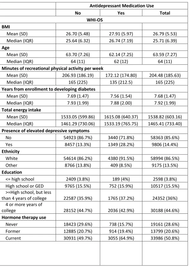
Table 1 presents the baseline characteristics of our study population, by antidepressant medication use. In both cohorts, the mean age was approximately 63 years old (63.59 (OS); 62.77 (CT)). Women were primarily White (86.5% (OS); 84.4% (CT)) and most had greater than high school education (80% (OS); 76.4% (CT)). Approximately 30% of women on antidepressants had elevated depressive symptoms (28.2% (OS); 29.8% (CT)). A greater percentage of
antidepressant medication users than non-users reported current use of hormone replacement therapy (64.9% vs. 49.7% (OS); 53.6% vs. 36.3% (CT)). Antidepressant users and non-users had approximately equal proportions that reported a family history of diabetes (30% vs. 30.6% (OS); 31.4% vs. 31.6% (CT)) or current smoking (7.2% vs. 5.4% (OS); 9.0% vs. 7.2% (CT)). Mean BMI was very similar for those on antidepressants vs. not (27.91 vs. 26.70 (OS); 29.41 vs. 28.48 (CT)).
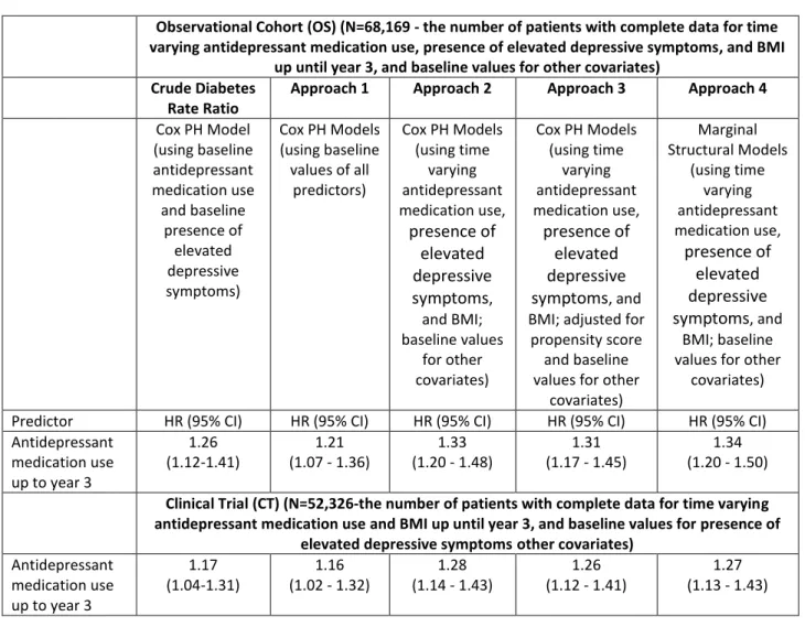
Table 2 presents development of diabetes for those who were exposed to
antidepressant medication compared to those who were not for all 4 modeling approaches. The Cox PH model including only baseline antidepressant medication use and baseline presence of elevated depressive symptoms produced a crude diabetes rate ratio of 1.26 (95% CI 1.12-1.41) indicating a significant increase in diabetes risk without adjusting for other factors. The standard Cox model in Approach 1 does not adjust for time-dependent confounding and yielded a hazard ratio of 1.21 (95% CI 1.07 – 1.36) in the OS cohort. The Cox models in Approach 2 and Approach 3 using time-varying antidepressant medication use, time-varying presence of elevated
depressive symptoms and time-varying BMI, yielded almost identical results (HR=1.33, 95% CI 1.20-1.48; HR=1.31; 95% CI 1.17 - 1.45, respectively) and showed an increased risk of developing diabetes relative to Approach 1. The hazard ratio and confidence interval for the marginal
13
structural Cox model (Approach 4) was almost identical to the extended Cox models in Approach 2 and Approach 3 (HR=1.34; 95% CI 1.20 - 1.50) demonstrating that, in this application, the marginal structural Cox model yielded similar results to the traditional extended Cox model. The confidence intervals for all 4 models overlap indicating the models are not significantly different than one another.
As in the WHI OS, all models in the WHI-CT showed a significant increase in diabetes risk for those exposed to antidepressant medications vs. those who were not. The crude diabetes rate ratio (HR=1.17, 95% CI 1.04-1.31) was very similar to the results in Approach 1. The hazard ratios and confidence intervals for Approaches 2, 3, and 4 were almost identical, and like the OS cohort the risk estimate is greater than in Approach 1, which did not adjust for time-dependent confounding (HR: 1.16;95% CI 1.02-1.32). By adjusting for time-dependent confounding, the hazard ratios for Approach 2 and Approach 3 increased from Approach 1 (HR=1.28, 95% CI 1.14-1.43; HR=1.26, 95% CI 1.12-1.41, respectively). The marginal structural model in Approach 4 again estimated a hazard ratio almost identical to that of the extended Cox models (HR=1.27, 95% CI 1.13-1.43). The confidence intervals for all 4 models overlap, indicating they are not significantly different from one another.
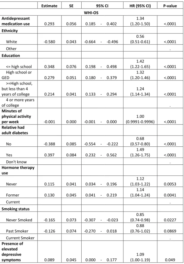
Table 3 presents the full model inverse probability of treatment-weighted estimates for the marginal structural models for the causal effect of antidepressant medication use on diabetes risk. All covariates including antidepressant medication use, ethnicity, education, minutes of physical activity per week, family history of diabetes, hormone therapy use, smoking status, presence of elevated depressive symptoms, BMI, age, and total energy intake are significant in the model for the WHI-OS, and all but total energy intake for the WHI-CT.
Table 4 presents the distributions of the IPTW weights, namely the estimated
14
time points. The probability of remaining uncensored was very close to 1 for both cohorts at each follow-up time point given both the baseline and time-varying covariates. There was variation in the probability of having one’s own observed treatment history, but the mean and median were very close to 1 at 36 month follow-up in the WHI-OS and 12 month follow-up in the WHI-CT.
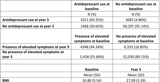
Table 5 presents an estimate of variation in the primary exposure and time-dependent confounder variables. Participants not on antidepressants remained pretty stable over time, but there was some switching on and off the drug. Of the 60,297 participants who were not taking antidepressants at baseline, 95% of them were also not taking them at year 3. Of the 3,321 participants who were taking antidepressants at baseline, 69.35% of them were also taking them at year 3. Approximately 30% of those who were on antidepressants at baseline were not taking them at year 3 and almost 5% of those not taking them at baseline were on
15
CHAPTER V DISCUSSION
We compared Marginal Structural Cox Proportional Hazards Models to standard Cox Models to estimate the association of antidepressant medication use and presence of elevated depressive symptoms on diabetes risk in the WHI. Previous research has shown a marginal structural modeling approach to be an unbiased method when you have a time-varying confounder, such as BMI, that is affected by previous exposure.
Our analyses did not find a difference in estimates between traditional Cox Proportional Hazards Models and Marginal Structural Cox Models in the WHI cohorts. The hazard ratios and confidence intervals for the 4 models we compared in the WHI OS and the 4 models we
compared in the WHI CT were all very similar. As our models increased in complexity, first taking into account the time-varying confounding (Cox PH Models) and then time-dependent confounding (Marginal Structural Models), the estimates were very similar to the crude rate ratio. This suggests that the time-varying confounders did not have much effect on our outcome. The confidence intervals overlapped, indicating they were not significantly different from one another. Our estimates of the IPTW weights were all very close to 1 which drives the observed similarity in results using marginal structural models when compared to Cox
Proportional Hazards Models.
A limitation of this work is that we had a limited amount of measurement points to work with in this dataset. The WHI-OS had 2 measurement time points. The WHI-CT had more time points available, but we were only able to utilize 3 of them because of insufficient numbers of participants with enough data for our main exposure variable after baseline. This allowed for long periods of time where we had no new information on their antidepressant medication use,
16
BMI, presence of elevated depressive symptoms, or other covariates. We may have missed important information on our time-varying exposure or covariates during that time. Participants could have gone off antidepressants 1 year after enrolling in the study, but we would not have accounted for that until year 3 when we had new data on that subject. Participants could also have gone off antidepressants and then gone back on during the period of time where we did not have new data. Because presence of elevated depressive symptoms was measured on only a small percentage of participants after baseline, our models for the WHI-CT could not use presence of elevated depressive symptoms as a time varying exposure.
Our analyses contribute to the literature by demonstrating that marginal structural models may not be required over traditional methods of analysis in all applications. A certain level of time-dependent confounding may need to exist in your dataset for these complicated methods to be called for. An important area for further study would be to assess what level of time-dependent confounding is necessary for marginal structural models to be a better approach than standard methods.
17
Table 1. Summary of Baseline Characteristics of the Study Sample (Continued on to next few pages)
Antidepressant Medication Use
No Yes Total WHI-OS BMI Mean (SD) 26.70 (5.48) 27.91 (5.97) 26.79 (5.53) Median (IQR) 25.64 (6.32) 26.74 (7.19) 25.71 (6.39) Age Mean (SD) 63.70 (7.26) 62.14 (7.25) 63.59 (7.27) Median (IQR) 64 (11) 62 (12) 64 (11)
Minutes of recreational physical activity per week
Mean (SD) 206.93 (186.19) 172.12 (174.80) 204.48 (185.63)
Median (IQR) 165 (225) 135 (212.5) 165 (225)
Years from enrollment to developing diabetes
Mean (SD) 7.69 (1.47) 7.56 (1.54) 7.68 (1.47)
Median (IQR) 7.93 (1.99) 7.88 (2.00) 7.92 (1.99)
Total energy intake
Mean (SD) 1533.05 (599.86) 1615.08 (640.37) 1538.82 (603.16) Median (IQR) 1461.29 (730.06) 1533.19 (765.75) 1465.41 (733.40)
Presence of elevated depressive symptoms
No 54923 (86.7%) 3440 (71.8%) 58363 (85.6%) Yes 8457 (13.3%) 1349 (28.2%) 9806 (14.4%) Ethnicity White 54614 (86.2%) 4380 (91.5%) 58994 (86.5%) Other 8766 (13.8%) 409 (8.5%) 9175 (13.5%) Education <= high school 2409 (3.8%) 189 (4%) 2598 (3.8%)
High school or GED 9765 (15.5%) 752 (15.9%) 10517 (15.5%) >=High school, but less
than 4 years of college 22587 (35.9%) 1765 (37.2%) 24352 (36%) 4 or more years of
college 28152 (44.7%) 2036 (42.9%) 30188 (44.6%)
Hormone therapy use
Never 18423 (29.6%) 738 (15.7%) 19161 (28.6%)
Former 12885 (20.7%) 914 (19.4%) 13799 (20.6%)
18
Antidepressant Medication Use
No Yes Total Family history of diabetes
No 41656 (66%) 3114 (65.2%) 44770 (65.9%) Yes 18923 (30%) 1463 (30.6%) 20386 (30%) Don't know 2569 (4.1%) 198 (4.1%) 2767 (4.1%) Smoking status Never Smoked 32614 (52%) 2188 (46.2%) 34802 (51.6%) Past Smoker 26685 (42.6%) 2207 (46.6%) 28892 (42.9%) Current Smoker 3370 (5.4%) 339 (7.2%) 3709 (5.5%) WHI-CT BMI Mean (SD) 28.48 (5.64) 29.41 (5.99) 28.54 (5.67) Median (IQR) 27.57 (7.20) 28.35 (7.96) 27.62 (7.23) Age Mean (SD) 62.83 (6.93) 61.77 (6.94) 62.77 (6.94) Median (IQR) 63 (11) 61 (11) 63 (11)
Minutes of recreational physical activity per week
Mean (SD) 163.22 (168.95) 138.94 (159.22) 161.72 (168.47)
Median (IQR) 125 (215) 85 (195) 120 (215)
Years from enrollment to developing diabetes
Mean (SD) 7.99 (1.68) 7.86 (1.73) 7.98 (1.68)
Median (IQR) 8.02 (1.73) 8.00 (1.91) 8.02 (1.76)
Total energy intake
Mean (SD) 1716.72 (679.54) 1819.65 (711.86) 1723.00 (682.00) Median (IQR) 1618.25 (832.50) 1716.34 (870.79) 1623.68 (833.68)
Presence of elevated depressive symptoms
No 42582 (86.7%) 2238 (70.2%) 44820 (85.7%) Yes 6557 (13.3%) 949 (29.8%) 7506 (14.3%) Ethnicity White 41243 (83.9%) 2924 (91.7%) 44167 (84.4%) Other 7896 (16.1%) 263 (8.3%) 8159 (15.6%) Education <= high school 2302 (4.7%) 144 (4.5%) 2446 (4.7%)
High school or GED 8991 (18.4%) 587 (18.5%) 9578 (18.4%) >=High school, but less
than 4 years of college 19110 (39.1%) 1236 (39%) 20346 (39.1%) 4 or more years of
19
Antidepressant Medication Use
No Yes Total Hormone therapy use
Never used hormones 17793 (37.9%) 662 (21.6%) 18455 (36.9%) Past hormone user 12122 (25.8%) 760 (24.8%) 12882 (25.7%) Current hormone user 17057 (36.3%) 1644 (53.6%) 18701 (37.4%)
Family history of diabetes
No 31282 (63.9%) 2022 (63.7%) 33304 (63.9%) Yes 15378 (31.4%) 1004 (31.6%) 16382 (31.4%) Don't know 2280 (4.7%) 147 (4.6%) 2427 (4.7%) Smoking status Never Smoked 25547 (52.5%) 1429 (45.2%) 26976 (52.1%) Past Smoker 19615 (40.3%) 1445 (45.7%) 21060 (40.6%) Current Smoker 3495 (7.2%) 285 (9%) 3780 (7.3%)
20
Table 2. Hazard Ratios Comparing Cox Proportional Hazards Models to Marginal Structural Models
Observational Cohort (OS) (N=68,169 - the number of patients with complete data for time varying antidepressant medication use, presence of elevated depressive symptoms, and BMI
up until year 3, and baseline values for other covariates) Crude Diabetes
Rate Ratio
Approach 1 Approach 2 Approach 3 Approach 4
Cox PH Model (using baseline antidepressant medication use and baseline presence of elevated depressive symptoms) Cox PH Models (using baseline values of all predictors) Cox PH Models (using time varying antidepressant medication use, presence of elevated depressive symptoms, and BMI; baseline values for other covariates) Cox PH Models (using time varying antidepressant medication use, presence of elevated depressive symptoms, and BMI; adjusted for
propensity score and baseline values for other
covariates) Marginal Structural Models (using time varying antidepressant medication use, presence of elevated depressive symptoms, and BMI; baseline values for other
covariates) Predictor HR (95% CI) HR (95% CI) HR (95% CI) HR (95% CI) HR (95% CI) Antidepressant medication use up to year 3 1.26 (1.12-1.41) 1.21 (1.07 - 1.36) 1.33 (1.20 - 1.48) 1.31 (1.17 - 1.45) 1.34 (1.20 - 1.50)
Clinical Trial (CT) (N=52,326-the number of patients with complete data for time varying antidepressant medication use and BMI up until year 3, and baseline values for presence of
elevated depressive symptomsother covariates)
Antidepressant medication use up to year 3 1.17 (1.04-1.31) 1.16 (1.02 - 1.32) 1.28 (1.14 - 1.43) 1.26 (1.12 - 1.41) 1.27 (1.13 - 1.43)
21
Table 3. Inverse Probability of Treatment-Weighted Estimates of The Parameters Of A Marginal Structural Model For The Causal Effect Of Antidepressant Medication Use On Diabetes Risk (Continued on to next few pages)
Estimate SE 95% CI HR (95% CI) P-value
WHI-OS Antidepressant medication use 0.293 0.056 0.185 - 0.402 1.34 (1.20-1.50) <.0001 Ethnicity White -0.580 0.043 -0.664 - -0.496 0.56 (0.51-0.61) <.0001 Other . Education <= high school 0.348 0.076 0.198 - 0.498 1.42 (1.22-1.65) <.0001 High school or GED 0.279 0.051 0.180 - 0.379 1.32 (1.20-1.46) <.0001 >=High school,
but less than 4
years of college 0.214 0.041 0.133 - 0.294 1.24 (1.14-1.34) <.0001 4 or more years of college . Minutes of physical activity per week -0.001 0.000 -0.001 - 0.000 1.00 (0.9991-0.9996) <.0001 Relative had adult diabetes No -0.388 0.085 -0.554 - -0.222 0.68 (0.57-0.80) <.0001 Yes 0.397 0.084 0.232 - 0.562 1.49 (1.26-1.75) <.0001 Don't know . Hormone therapy use Never 0.115 0.041 0.034 - 0.196 1.12 (1.03-1.22) 0.0053 Former 0.130 0.045 0.041 - 0.219 1.14 (1.04-1.24) 0.0041 Current . Smoking status Never Smoked -0.165 0.073 -0.307 - -0.023 0.85 (0.74-0.98) 0.0227 Past Smoker -0.126 0.074 -0.270 - 0.018 0.88 (0.76-1.02) 0.0869 Current Smoker . Presence of elevated depressive symptoms 0.089 0.045 0.000 - 0.177 1.09 (1.00-1.19) 0.049
22
Estimate SE 95% CI HR (95% CI) P-value
BMI 0.080 0.002 0.076 - 0.084 1.08 (1.08-1.09) <.0001 Age 0.018 0.003 0.013 - 0.023 1.02 (1.01-1.02) <.0001 Baseline total energy intake 4.87- 1100.54 -0.205 0.048 -0.300 - -0.110 0.81 (0.74-0.90) <.0001 1100.55- 1437.42 -0.238 0.049 -0.333 - -0.143 0.79 (0.72-0.87) <.0001 1437.44- 1828.01 -0.174 0.048 -0.268 - -0.080 0.84 (0.76-0.92) 0.0003 >=1828.02 WHI-CT Antidepressant medication use 0.242 0.059 0.126 - 0.357 1.27 (1.13-1.43) <.0001 Ethnicity White -0.462 0.041 -0.542 - -0.381 0.63 (0.58-0.68) <.0001 Other Education <= high school 0.315 0.072 0.174 - 0.455 1.37 (1.19-1.58) <.0001 High school or GED 0.196 0.049 0.101 - 0.292 1.22 (1.11-1.34) <.0001 >=High school,
but less than 4
years of college 0.219 0.041 0.139 - 0.298 1.24 (1.15-1.35) <.0001 4 or more years of college Minutes of physical activity per week -0.001 0.000 -0.001 - 0.000 0.999 (0.999-1.00) <.0001 Relative had adult diabetes No -0.358 0.075 -0.505 - -0.210 0.70 (0.60-0.81) <.0001 Yes 0.323 0.074 0.177 - 0.468 1.38 (1.19-1.60) <.0001 Don't know Hormone therapy use Never 0.167 0.045 0.078 - 0.255 1.18 (1.08-1.29) 0.0002 Former 0.165 0.049 0.069 - 0.261 1.18 (1.07-1.30) 0.0008 Current
23
Estimate SE 95% CI HR (95% CI) P-value
Smoking status Never Smoked -0.186 0.063 -0.310 - -0.062 0.83 (0.73-0.94) 0.0033 Past Smoker -0.203 0.065 -0.330 - -0.076 0.82 (0.72-0.93) 0.0018 Current Smoker Presence of elevated depressive symptoms 0.088 0.045 0.000 - 0.176 1.09 (1.00-1.19) 0.0511 BMI 0.073 0.002 0.069 - 0.077 1.08 (1.07-1.08) <.0001 Age 0.020 0.003 0.015 - 0.025 1.02 (1.02-1.03) <.0001 Baseline total energy intake 4.87- 1100.54 -0.037 0.049 -0.133 - 0.059 0.96 (0.88-1.06) 0.4477 1100.55- 1437.42 -0.037 0.046 -0.127 - 0.053 0.96 (0.88-1.05) 0.4167 1437.44- 1828.01 -0.060 0.044 -0.146 - 0.026 0.94 (0.86-1.03) 0.17 1828.02- 23020.93 Participated in hormone therapy trial 0.096 0.052 -0.006 - 0.198 1.10 (0.99-1.22) 0.0656 Participated in dietary modification trial 0.095 0.054 -0.010 - 0.201 1.10 (0.99-1.22) 0.0756 Participated in calcium/ vitamin D supplementation -0.028 0.034 -0.095 - 0.039 0.97 (0.91-1.04) 0.4128
24
Table 4. EstimatedProbability of Having One’s Own Observed Treatment History And Censoring History At Follow-Up
N Mean SD Median
Quartile
Range Minimum Maximum
WHI-OS 36 Months
Probability of having observed antidepressant medication history given baseline covariates 64048 0.91 0.05 0.92 0.06 0.48 0.99 given time-varying covariates 64048 0.91 0.06 0.92 0.06 0.36 0.99
Probability of being uncensored given baseline covariates 64099 0.99983 0.0000261 0.9998269 0.0000372 0.99968 0.99988 given time-varying covariates 64099 0.99983 0.0000262 0.9998270 0.0000374 0.99969 0.99988 WHI-CT 12 Months
Probability of having observed antidepressant medication history given baseline
covariates 46084 0.93 0.04 0.95 0.05 0.52 0.99 given time-varying
covariates 46084 0.93 0.05 0.95 0.05 0.31 0.99 Probability of being uncensored
given baseline covariates 46084 0.9999997 6.4192736E-8 0.9999997 8.7696349E-8 0.9999994 0.9999998 given time-varying covariates 46084 0.9999997 6.4550241E-8 0.9999997 8.8088701E-8 0.9999993 0.9999998 36 Months
Probability of having observed antidepressant medication history given baseline covariates 45235 0.86 0.09 0.88 0.10 0.25 0.99 given time-varying covariates 45235 0.86 0.09 0.88 0.10 0.20 0.99 Probability of being uncensored
given baseline covariates 45235 0.999971 6.4295277E-6 0.999972 8.8005442E-6 0.99994 0.99998 given time-varying covariates 45235 0.999971 6.4828669E-6 0.999972 8.8476766E-6 0.99993 0.99998
25
Table 5. Estimate of Variation in Primary Exposure and Time-Dependent Confounder Variables (WHI-OS) Antidepressant use at baseline No antidepressant use at baseline N (%) N (%)
Antidepressant use at year 3 3321 (69.35%) 3083 (4.86%)
No antidepressant use at year 3 1468 (30.65%) 60,297 (95.14%)
Presence of elevated symptoms at baseline
No presence of elevated symptoms at baseline Presence of elevated symptoms at year 3 4348 (44.34%) 6,333 (10.85%)
No presence of elevated symptoms at
year 3 5,458 (55.66%) 52,030 (89.15%)
Baseline Year 3
Mean (SD) Mean (SD)
26
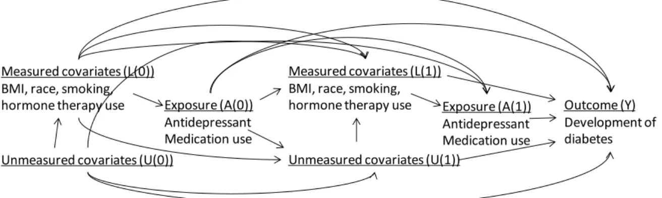
Figure 1. Illustration of time-dependent confounding by BMI in the association of antidepressant medication use and time to development of diabetes
Figure 1 illustrates the hypothesis that there is time-varying confounding by BMI with regard to the association between diabetes risk and antidepressant use. Let A denote the exposure or antidepressant use, L denotes measured covariates such as BMI or race, U denotes unmeasured covariates and Y denotes the outcome of development of diabetes. The causal graph in Figure 1 shows that the probability of antidepressant medication use (A) depends on BMI (L), but not U. There is confounding, but measured covariates are sufficient to adjust for, so no unmeasured confounding. The probability of antidepressant medication use at baseline (A(0)) is determined by baseline BMI (L(0)). In our example, confounding is time dependent because antidepressant medication use vs. non-use at time 1 (A(1)) is determined by previous exposure (A(0)) and BMI at time 1 (L(1)). Even though antidepressant medication use (A) and diabetes (Y) share common causes, the non-causal association between exposure and outcome can be blocked by
conditioning on the BMI (L). Measured covariates (L(0)) BMI, race, smoking, hormone therapy use
Unmeasured covariates (U(0))
Exposure (A(0)) Antidepressant Medication use Outcome (Y) Development of diabetes Measured covariates (L(1))
BMI, race, smoking, hormone therapy use
Unmeasured covariates (U(1))
Exposure (A(1)) Antidepressant Medication use
27
Figure 2. Flow chart describing analytic cohort included for the investigation
Exclusions:
377 women without race/ethnicity information
7,167 women with self-reported DM at baseline (3,902 from the WHI-OS arm and 3,265 from the CT arm respectively).
145 women missing DM at baseline
CT arm: 64,706 OS arm: 89,413 161,808 Total 154,119 Enrolled 64,175 women with nonmissing information 3624 self reported diabetes 531 women missing baseline depression 4171 self reported diabetes 10427 women missing depression at baseline or 3 year followup 78986 women with nonmissing depression at baseline and 3 year visit
55,206 women with nonmissing information 8969 women missing anti depression medication at baseline, 1 year or 3 year followup 74792 women with nonmissing information 4194 women missing anti depression medication at baseline or 3 year followup 68,169 women 3 year visit within ½ year of 3 year mark [913-1278 days from enrollment] 3918 women 3
year visit more than ½ year from 3 years post enrollment date 52,326 women with nonmissing information 2880 women missing BMI at baseline, 1 year or 3 year followup 72,087 women with nonmissing information 2705 women missing BMI at baseline, 1 year or 3 year followup
28
APPENDIX
SAS CODE TO FIT THE MARGINAL STRUCTURAL COX PROPORTIONAL HAZARDS MODEL
Here I provide details on how to set up the data, along with some SAS code to perform the Marginal Structural Cox Proportional Hazards analysis. The first part of the analysis uses the proc logistic procedure to calculate the probability of not being on antidepressants (Models 1 and 2). Data in the file ‘iptw’ contains 1 record per woman for each time point included in the analysis. For example, in the WHI-OS dataset, we have measurements at baseline and year 3. Each woman has two records, one for baseline and one for year 3. Next we use the proc logistic procedure to calculate the probability of not being censored (Models 3 and 4). In the data file ‘iptw2’ the data has been expanded so that a woman has 1 record per month until her time to diabetes or time to censoring. The dataset ‘main’ merges Models 1-4 together to calculate our IPTW weights. This again will be an expanded dataset so a woman has 1 record per month until her time to diabetes or time to censoring. The dataset ‘main_w’ contains the inverse probability of treatment weights and is the dataset used to run the marginal structural model analysis. Last, we use the proc genmod procedure to fit the final pooled logistic regression model to obtain the estimates of our association of interest.
At the baseline time point, the variables in Model 1 are basically a subset of Model2. Model 1 includes only baseline covariates and Model 2 includes baseline and follow-up values for the same variables. Because baseline is the start of our analysis, there are no follow-up values to consider at that time point. For that reason, the weights at baseline are going to be 1 and here we run a logistic regression model estimating the probability of not being on
29
Antidep is a dichotomous 0/1 indicator of the participant being on or off
antidepressants. Model 1 includes a time-dependent intercept and baseline covariates: presence of elevated depressive symptoms (base_depression), BMI (base_bmi), Age
(age), Ethnicity (ethnic_cat), Education (educ4), Minutes of physical activity per week (tminwk), Total energy intake (base_energy_cat), Family history of diabetes
(diabrel), Hormone therapy use (hormstat) and smoking status (smoking). Model 2 includes a time-dependent intercept and baseline covariates, with the addition of the most recent time-dependent values (depression, bmi).
The outcome variable in Models 3 and 4 is a dichotomous indicator of whether or not the participant has been censored up to that time point. These models include as regressors variables for ‘month’ and ‘month2’ to relax the linearity assumption. All available person months are included. Model 3 includes baseline covariates with the addition of baseline antidepressant medication use, while Model 4 includes the baseline covariates as well as the most recent time-dependent value.
We merge Models 1-4 together and in the following data step use the predicted values from those models to compute our IPTW estimates. First, we calculate the numerator K2_0 and denominator K1_0 of the probability of not being censored by forming the product up to month
t of the subject-specific values predicted in Models 3 and 4.
We then calculate the numerator K1_0 and denominator K2_0 of the probability of not being on antidepressants by forming the product up to month t of the subject-specific values predicted in Models 1 and 2. We multiply by that probability for participants who were not on antidepressants and 1-that probability for participants who were taking antidepressants from month 36 until time to diabetes or time to censoring. From baseline until month 35, the
30
of the probability of not being censored and the probability of not being on antidepressants to calculate the ‘stabilized’ (stabw) and ‘non-stabilized’ (nstabw) weights.
In our last step, we use the proc genmod procedure to fit the weighted pooled logistic model to obtain estimates of our association of interest from our Marginal Structural Cox PH Model. The outcome here is diabetes_tv which is a dichotomous indicator of whether or not the participant developed diabetes during that month. The patient ID variable and the
independent working correlation matrix (subject=id/type=ind) must be specified. We weighted the model used the stabilized weights by using the ‘scwgt stabw’ statement in the procedure. The ‘estimate’ statement asks the procedure to report the odds ratio for our main association of interest which we use as our hazard ratio, in addition to the coefficients in the model.
/*calculate probability of not being on antidepressants*/ /* Model 1*/
proc sort data=iptw;
by id month;
run;
proc logistic data=iptw;
class ethnic_cat educ4 base_energy_cat hormstat smoking diabrel;
where month=36;
model antidep=base_depression base_bmi age ethnic_cat educ4 tminwk base_energy_cat diabrel hormstat smoking;
output out=model1 p=pandep_0_temp;
run;
/* Model 2*/
proc logistic data=iptw;
where month=36;
class ethnic_cat educ4 base_energy_cat energy_cat hormstat smoking base_energy_cat diabrel;
model antidep=base_depression depression base_bmi bmi age ethnic_cat educ4 tminwk base_energy_cat diabrel hormstat smoking;
output out=model2 p=pandep_w_temp;
run;
31 /* Model 3*/
proc logistic data=iptw2;
class ethnic_cat educ4 base_energy_cat hormstat smoking diabrel;
model censor_tv=antidep depression bmi age ethnic_cat educ4 tminwk base_energy_cat diabrel hormstat smoking month month_sq;
output out=model3 p=punc_0;
run;
/* Model 4*/
proc logistic data=iptw2;
class ethnic_cat educ4 base_energy_cat hormstat smoking diabrel;
model censor_tv=antidep antidepressant_tv depression bmi age ethnic_cat educ4 tminwk base_energy_cat diabrel hormstat smoking depression_tv bmi_tv month month_sq;
output out=model4 p=punc_w;
run;
/*merge data*/
data main;
merge temp1 temp2 model3(in=a) model4(in=b);
by id month; if a=1 and b=1; if first.id then do; pandep_0 = 1; pandep_w = 1; end; if month=36 then do; pandep_0=pandep_0_temp; pandep_w=pandep_w_temp; end;
retain pandep_0 pandep_w;
run;
/* Calculate the weights*/
data main_w;
set main;
by id month;
/*reset variables for a new patient*/ if first.id then do;
k2_0=1; k2_w=1;
end;
retain k2_0 k2_w;
/*inverse probability of censoring weights*/ else do;
k2_0=k2_0*punc_0; k2_w=k2_w*punc_w;
32
/* Inverse probability of treatment weights */
if antidepressant_tv=0 and month>=36 then k1_0=pandep_0;
if antidepressant_tv=0 and month>=36 then k1_w=pandep_w;
if antidepressant_tv=1 and month>=36 then k1_0=(1-pandep_0);
if antidepressant_tv=1 and month>=36 then k1_w=(1-pandep_w);
if month<36 then k1_0=1;
if month<36 then k1_w=1;
/* Stabilized and non stabilized weights */
stabw=(k1_0*k2_0)/(k1_w*k2_w); nstabw=1/(k1_w*k2_w);
run;
/* Pooled logistic regression model to run the MSM analysis */
proc genmod data=main_w descending;
class id ethnic_cat educ4 hormstat smoking base_energy_cat diabrel;
model diabetes_tv=antidepressant_tv ethnic_cat educ4 tminwk diabrel hormstat smoking depression_tv bmi_tv age base_energy_cat month month_sq/ link=logit dist=bin;
scwgt stabw;
repeated subject=id/ type=ind;
estimate "log O.R. antidepressant" antidepressant_tv 1 / exp;
33
REFERENCES
1. Kim CK, McGorray SP, Bartholomew BA, et al. Depressive symptoms and heart rate variability in postmenopausal women. Arch Intern Med. 2005 Jun 13;165(11):1239-44. 2. Wild S, Roglic G, Green A, Sicree R, King H. Global prevalence of diabetes: estimates for
the year 2000 and projections for 2030. Diabetes Care. 2004 May;27(5):1047-53. 3. Anderson RJ, Freedland KE, Clouse RE, Lustman PJ. The prevalence of comorbid
depression in adults with diabetes: a meta-analysis. Diabetes Care. 2001 Jun;24(6):1069-78.
4. Knol MJ, Twisk JW, Beekman AT, Heine RJ, Snoek FJ, Pouwer F. Depression as a risk factor for the onset of type 2 diabetes mellitus. A meta-analysis. Diabetologia. 2006 May;49(5):837-45.
5. Mezuk B, Eaton WW, Albrecht S, Golden SH. Depression and type 2 diabetes over the lifespan: a meta-analysis. Diabetes Care. 2008 Dec;31(12):2383-90.
6. Atlantis E, Browning C, Sims J, Kendig H. Diabetes incidence associated with depression and antidepressants in the Melbourne Longitudinal Studies on Healthy Ageing
(MELSHA). Int J Geriatr Psychiatry. 2009 Jul;25(7):688-96.
7. Brown LC, Majumdar SR, Johnson JA. Type of antidepressant therapy and risk of type 2 diabetes in people with depression. Diabetes Res Clin Pract. 2008 Jan;79(1):61-7. 8. Rubin RR, Ma Y, Marrero DG, et al. Elevated depression symptoms, antidepressant
medicine use, and risk of developing diabetes during the diabetes prevention program. Diabetes Care. 2008 Mar;31(3):420-6.
9. Andersohn F, Schade R, Suissa S, Garbe E. Long-term use of antidepressants for depressive disorders and the risk of diabetes mellitus. Am J Psychiatry. 2009 May;166(5):591-8.
10. Campayo A, de Jonge P, Roy JF, et al. Depressive disorder and incident diabetes mellitus: the effect of characteristics of depression. Am J Psychiatry. 2010 May;167(5):580-8. 11. Olfson M, Marcus SC. National patterns in antidepressant medication treatment. Arch
Gen Psychiatry. 2009 Aug;66(8):848-56.
12. The Medicated Americans: Antidepressant Prescriptions on the Rise July 15, 2013; Available from: http://www.sciam.com/article.cfm?id=the-medicated-americans. 13. Ma Y, Balasubramanian R, Pagoto SL, et al. Elevated depressive symptoms,
antidepressant use, and diabetes in a large multiethnic national sample of postmenopausal women. Diabetes Care. 2011 Nov;34(11):2390-2.
14. Hernan MA, Brumback B, Robins JM. Marginal structural models to estimate the causal effect of zidovudine on the survival of HIV-positive men. Epidemiology. 2000
Sep;11(5):561-70.
15. Robins JM, Hernan MA, Brumback B. Marginal structural models and causal inference in epidemiology. Epidemiology. 2000 Sep;11(5):550-60.
16. Robins JM. Causal inference from complex longitudinal data. In: Berkane M, editor. Latent Variable Modeling and Applications to Causality Lecture Notes in Statistics (120). New York, NY: Springer Verlag; 1997. p. 69-117.
17. Design of the Women's Health Initiative clinical trial and observational study. The Women's Health Initiative Study Group. Control Clin Trials. 1998 Feb;19(1):61-109.
34
18. Ritenbaugh C, Patterson RE, Chlebowski RT, et al. The Women's Health Initiative Dietary Modification trial: overview and baseline characteristics of participants. Ann Epidemiol. 2003 Oct;13(9 Suppl):S87-97.
19. Stefanick ML, Cochrane BB, Hsia J, Barad DH, Liu JH, Johnson SR. The Women's Health Initiative postmenopausal hormone trials: overview and baseline characteristics of participants. Ann Epidemiol. 2003 Oct;13(9 Suppl):S78-86.
20. Langer RD, White E, Lewis CE, Kotchen JM, Hendrix SL, Trevisan M. The Women's Health Initiative Observational Study: baseline characteristics of participants and reliability of baseline measures. Ann Epidemiol. 2003 Oct;13(9 Suppl):S107-21.
21. Margolis KL, Lihong Q, Brzyski R, et al. Validity of diabetes self-reports in the Women's Health Initiative: comparison with medication inventories and fasting glucose