Exploring Structural Consistency in Graph
Regularized Joint Spectral-Spatial Sparse Coding
for Hyperspectral Image Classification
Changhong Liu, Jun Zhou,
Senior Member, IEEE,
Jie Liang, Yuntao Qian,
Member, IEEE,
Hanxi Li,
and Yongsheng Gao,
Senior Member, IEEE
Abstract—In hyperspectral image classification, both spec-tral and spatial data distributions are important in describing and identifying different materials and objects in the image. Furthermore, consistent spatial structures across bands can be useful in capturing inherent structural information of objects. These imply that three properties should be considered when reconstructing an image using sparse coding methods. Firstly, the distribution of different ground objects leads to different coding coefficients across the spatial locations. Secondly, local spatial structures change slightly across bands due to different reflectance properties of various object materials. Lastly and more importantly, some sort of structural consistency shall be enforced across bands to reflect the fact that the same object appears at the same spatial location in all bands of an image. Based on these considerations, we propose a novel joint spectral-spatial sparse coding model that explores structural consistency for hyperspectral image classification. For each band image, we adopt a sparse coding step to reconstruct the structures in the band image. This allows different dictionaries be generated to characterize the band-wise image variation. At the same time, we enforce the same coding coefficients at the same spatial location in different bands so as to maintain consistent structures across bands. To further promote the discriminating power of the model, we incorporate a graph Laplacian sparsity constraint into the model to ensure spectral consistency in the dictionary generation step. Experimental results show that the proposed method outperforms some state-of-the-art spectral-spatial sparse coding methods.
Index Terms—Hyperspectral image, structural consistency, sparse coding, graph Laplacian regularizer.
I. INTRODUCTION
Remote sensing hyperspectral images (HSI) are acquired in hundreds of bands to measure the reflectance of earth surface, discriminate various materials, and classify ground objects. HSI classification aims at assigning each pixel with
C. Liu and H. Li are with the School of Computer and Information Engineering, Jiangxi Normal University, Nanchang, 330022, China.
J. Zhou is with the School of Information and Communication Technol-ogy, Griffith University, Nathan, Australia. Corresponding author: J. Zhou ([email protected])
J. Liang is with the School of Engineering, the Australian National University, Canberra, Australia.
Y. Qian is with the Institute of Artificial Intelligence, College of Computer Science, Zhejiang University, Hangzhou, 310027, China.
Y. Gao is with the School of Engineering, Griffith University, Nathan, Australia.
This work was supported by the Australian Research Council Linkage Project (No. LP150100658), the National Natural Science Foundation of China (No. 61571393, 61462042, 61365002, 61262036), and the Visiting Scholars Special Funds from Young and Middle-aged Teachers Development Program for Universities in Jiangxi Province.
one thematic class in a scene [1]. Various machine learning models have been proposed for this purpose, such as Bayesian model [1], random forest [2], neural networks [3], support vector machines (SVM) [4]–[7], sparse representation [8]– [13], and deep learning [14], [15].
Many HSI classification methods make prediction based on the spectral response at a single pixel [6], [8], [9], [16]–[19]. While spectral information is essential in image classification and material identification, information extracted from spatial domain is very useful to discriminate various targets made of the same materials [20], [21]. To address this need, spectral-spatial HSI classification approaches have been reported, each type of approach exploring and exploiting different ways to integrate spatial features with spectral features. Mura et al. and Ghamisi et al. proposed mathematical morphology methods to analyze spatial relationships between pixels using structured elements [22], [23]. Markov random field methods considered spatial information by adding to the objective function a term that defines spatial correlations in the prior model [24], [25]. Qian et al. developed 3D discrete wavelet transform to extract 3D features along spectral and spatial dimensions simultaneously [26]. Moreover, many researchers proposed sparse representation methods to include spatial sparsity constraints or kernel function to integrate spectral and spatial features [10], [12], [27]–[31].
Among these approaches, sparse representation based clas-sifiers have achieved the state-of-the-art performance [27], [32]. They provide an effective way of modelling the spatial neighborhood relationship and the distribution of atoms in the spectral or spatial domain, so that both spectral and spatial information can be seamlessly integrated and modeled. In sparse representation, a test sample is treated as a linear combination of atoms from training samples or a learned dictionary. A sparse regularization term is normally included to learn a discriminative representation of images [33]–[35]. Recently, structured sparsity priors are also incorporated into reconstruction methods [12], [36]–[39]. These include joint sparsity constraint [40], group sparsity constrain [41], graph Laplacian sparsity constraint [36], low-rank constraint [42], and low-rank group sparsity constraint [12]. Graph Laplacian sparsity constraint is based on the spatial dependencies be-tween the neighboring pixels [12], [36]. It preserves the local manifold structure so that if two data points are close in their original data space, the sparse representations of these two data points are also close to each other in the new data space.
Band 6 Band 15 Band 32 Band 45 Band 80 Band 100
(a)
(b)
(c)
(d)
Fig. 1. Consistent structures in the University of Pavia dataset. (a) Pixel (362, 149) in bands 6, 15, 32, 45, 80 and 100 for the “Bitumen” class. (b)13×13 patches centered at pixel (362, 149). (c) Pixel (251, 76) in bands 6, 15, 32, 45, 80 and 100 for the “Bricks” class. (d)13×13patches centered at pixel (251, 76).
Although spectral-spatial analysis has been studied inten-sively in HSI classification, how to explore the local structural information has not been adequately addressed. To get a deeper understanding of the structural information embedded in a hyperspectral image, we use the University of Pavia image in Fig. 1 as an example. In the first row, bands 6, 15, 32, 45, 80 and 100 are displayed. In the second and fourth rows, small patches extracted from neighborhoods around pixels (362, 149) and (251, 76) are displayed, respectively. Three observations can be obtained from this figure. Firstly, various land cover classes have different distributions in the spatial domain. This happens in all bands. Secondly, local spatial structures change slightly across different bands. This is due to the distinct reflectance properties of object materials at different light wavelength. As a consequence, the extracted Gabor features at the same location in different bands also change slightly. Lastly and more importantly, some sort of structural consistency can be observed across bands, as the ground objects at each location are consistent in all bands. Such consistency has been proved to be useful in hyperspec-tral image denoising [43]. In general, image representation and classification models shall be able to address all these observations.
Motivated by the above observations, we propose a novel joint spectral-spatial framework to explore structural consis-tency along all bands in the sparse coding model. For each band image, image patches or 2D image features centered at pixels are firstly extracted from local neighborhood, which contain local structures of the central pixels. Then a sparse coding step is adopted to reconstruct the structures in the band images. This allows different dictionaries be generated to characterize the band-wise image variation. At the same time, consistent structures across bands are maintained by enforcing the same coding coefficients at the same spatial location in different bands. To further promote the discriminating power of the model, a graph Laplacian sparsity constraint is incor-porated into the model to ensure spectral consistency in the dictionary generation step. At last, the learned coefficients are fed into the classifier for pixel-wise classification.
The contribution of this paper lies in two aspects. First, we propose a novel joint spectral-spatial sparse coding framework, which can explore the structural consistency along all bands and integrate the spectral information and spatial structures into a sparse coding framework. Under this framework, 2D structural features can be applied to HSI classification effec-tively and directly, and the learned coefficients inherently
con-tain both spectral characteristics and spatial structures of HSI images. Second, we extend this model by including a graph regularization term to preserve the spectral relations between data points. This allows better relationship between data be modelled, which improves the classification performance.
The rest of this paper is organized as follows. In Section II, we review related work on sparse representation based hyper-spectral image classification. In Section III, we first briefly introduce the basic sparse coding model. Then we describe the proposed method that preserves structural consistency, its graph-based extension, and the optimization algorithm for learning sparse coefficient and dictionaries. Experimental results are presented in Section IV. We conclude our work and point out future research direction in Section V.
II. RELATED WORK
Recently, sparse representation has been widely used in HSI classification. It allows spectral information be combined with spatial information, so that discriminative image representation can be achieved. Some of them directly extract the spectral-spatial features and then feed these features into the sparse representation model. Qianet al.extracted a three-dimensional discrete wavelet transform (3D-DWT) texture features to cap-ture geometrical and statistical spectral-spatial struccap-tures and then applied them to the sparse representation model [26]. He et al. proposed an l1 minimization based spectral-spatial
classification method. A spatial translation invariant wavelet sparse representation [13] was adopted in the model. Yang
et al. combined Gabor spatial features and nonparametric weighted spectral features, and then applied sparse repre-sentation to describe the HSI [11]. To selected the most representative Gabor cube features for image classification, Jia et al.proposed to use Fisher discrimination criterion and a multi-task joint sparse representation framework [31].
Structured sparsity constraints [12], [36], [40]–[42] are often incorporated into sparse representation to improve the performance of HSI classification. These methods explore the spatial dependencies between neighboring pixels, or the inherent structure of dictionary, or both [12]. For example, Laplacian constraint has been incorporated into the sparse recovery optimization problem such that the reconstructed neighboring pixels have similar spectral characteristics [44]. In [26], Qian et al.used sparsity constraints to help selecting the discriminant features from a pool of 3D-DWT texture fea-tures. Low rank sparse representation methods have also been proposed to explore the spatial correlations of neighboring pixels [12], [45].
The sparse representation is further extended into kernelized or joint sparse form to exploit the spatial correlation across neighboring pixels. Chen et al. used simultaneous subspace pursuit (SSP) method, simultaneous orthogonal matching pur-suit (SOMP), and their kernelized extension for spectral-spatial HSI classification [10], [44]. He et al. utilized empirical mode decomposition and morphological wavelet transform to extract spectral-spatial features which were then integrated by a sparse multi-task learning method [28]. Liuet al.proposed a neighboring filtering kernel sparse representation for enhanced
classification of HSIs [27]. The relationship between pixels in a local neighborhood can also be modeled by structural simi-larity [29], graph embedding [32], and set-to-set distance [46]. When joint sparse representation is concerned, Zhang et al.
constructed multiple features and enforced pixels in a small region to share the same sparsity pattern for each type of feature [47]. Wanget al.presented a spatial-spectral derivative-aided kernel joint sparse representation, which considered high order spatial context and distinct spectral information [30].
Most aforementioned methods combine spectral information with spatial information using spatial constraints, complex spectral-spatial features, or joint sparse form of neighborhood pixels, and then make classification by minimizing the residual between a testing sample and the reconstructed image. Unlike the sparse representation procedure, Farani and Rabiee [48] proposed a sparse coding method for HSI classification, which used a spatially weighted sparse unmixing approach as a front-end and the learned sparse codes as the input to a linear SVM. Similar to this work, in our method, we also use learned sparse codes as inputs to the the classifier. This is done by firstly extracting 2D spatial features from local neighborhoods and the learning band-wise distinct dictionary. Finally we force the same spatial location in different bands share the same coding coefficients to capture the structural consistency along all bands.
III. SPARSECODING WITHSTRUCTURALCONSISTENCY FORHSI CLASSIFICATION
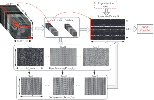
In an HSI, the distributions of spatial structures vary in different spatial locations, but are closely related to each other in different bands. Such structural consistency has been shown in Fig. 1. Considering the spatial correlation along the spectral dimension, we construct a joint spectral-spatial sparse coding model with structural consistency by assigning the same coefficient in the same position of different bands. The modelling process also preserves the distinct band character-istics by producing band-wise dictionaries. The framework of the proposed sparse coding with structural consistency method is shown in Fig. 2.
At each pixel, local spatial feature is firstly extracted band by band. Though any type of 2D feature can be used here, we adopted a simple solution by extracting image patch centered at the pixel. Then the dictionaries on all bands are trained in-dividually and simultaneously with the same coefficient across bands. That is to say, theb-th dictionary is learned only using the spatial features extracted from theb-th band and there are
B different dictionaries for B bands of HSI. These learned dictionaries are then used to estimate a sparse coefficient for each pixel. The dictionary and coefficient are optimized iteratively until convergence. Finally, the sparse coefficients are fed into SVM for classifier learning or classification. The whole process includes two stages: training and testing. In the training stage, the dictionaries are learned using the training samples without using the class label information. Then the sparse coefficients of these samples are calculated and used to train the SVM classifier on labelled training samples. In the testing stage, the sparse coefficients are firstly calculated for
B =200 ǂ×ǂ Patches HSI Dictionaries {D1, 噯,DB} Sparse coefficient S
Band 1 Band b Band B
N R M R Width = 145 H eigh t = 14 5 Data Features{F1, 噯,FB}
Band 1 Band b Band B
N M_train Regularization term SVM Classifier
Fig. 2. The framework of the proposed method.Mis the total number of samples andM trainis the number of training samples to train the dictionaries
the testing samples using the learned dictionaries and are then fed into the SVM classifier for prediction.
A. Sparse Coding for Single-band Image
An HSI is a 3D structure and each band is a 2D image, so the sparse coding model of single band image can be generated following the general image sparse coding methods. In order to describe the spatial relationships between neighbourhoods, a√N×√N patch is extracted at each pixel and then reshaped into an N×1 vector. Then theb-th band HSI can be denoted as Fb = [fb1,· · · ,fbM] ∈ RN×M where M denotes the number of pixels. Let Db = [db1,· · ·,dbR] ∈ RN×R be the dictionary matrix of theb-th band where eachdbi denotes a basis vector in the dictionary, andR is the number of basis vector. Let Sb= [sb1,· · · ,sbM] ∈ RR×M be the coefficient matrix, where each column is a sparse coefficient for a pixel. The neighborhood feature of each pixelfbican be represented as a sparse linear combination of the basis vectors in the dictionary. The sparse coefficient of fbi can be obtained by minimizing the loss function with an`1regularizer as follows:
min Db,sbi kfbi−Dbsbik 2 +βksbik1 s.t.kdbik ≤c, i= 1,· · ·, R (1) whereβis the regularization parameter controlling the degree of sparsity and cis a constant. By summing up the loss func-tions at each pixel, we can formulate the objective function of the b-th band image as
min Db,Sb kFb−DbSbk 2 +βkSbk1 s.t.kdbik ≤c, i= 1,· · · , R (2)
This problem can be solved by alternatively optimizing basis vectors Db and coefficients Sb while fixing the other. For
Sb, the optimization can be solved by optimizing over each coefficient sbi individually. This is an `1 norm regularized
linear regression problem, so it can be solved efficiently by many optimization algorithms such as the feature-sign algorithm [49]. Fixing Db, the optimization becomes a least square problem with quadratic constraints and can be treated by the Lagrange dual as used in [49].
B. Structural Consistency across Bands
The goal of the sparse coding with structural consistency method is to maintain the distinct band characteristics while maintaining a consistent structure across bands. While sounds contradictory, we get this done by different treatments to the dictionary learning and sparse coefficients estimation which are two key components in sparse coding. To be more specific, different dictionaries are generated for different bands, so as to guarantee that the band-wise variation of spectral reflectance of materials can be accurately described. At the same time, we enforce the same coefficient in all bands when reconstructing a band image from the corresponding band specific dictionary. LetF= [F1,· · ·,FB]be the set of data extracted from an HSI, whereB is the number of bands.Fb= [fb1,· · ·,fbM] ∈ RN×M is the set of features extracted from the b-th band, where M is the number of pixels and N is the dimension of data. Note that the data at a pixel is extracted from a local neighborhood, either in the form of raw intensity values as in Section III-A, or certain image features such as discrete wavelet and so on. Then we formulate the structural
consistency model for the whole HSI as min D1,···,DB,S B X b=1 kFb−DbSk 2 +βkSk1 s.t.kdbik ≤c, i= 1,· · ·, R, b= 1,· · · , B (3)
whereD1,· · ·,DB ∈RN×Rare the dictionaries for different bands, R is the size of dictionary, and S ∈ RR×M is the sparse coefficient matrix, which is the same for all bands.
C. Extension with Graph Constraint
In order to capture the structural relationship between the neighboring pixels and improve the discriminative capability of the learned model, sparse coding models are usually added with certain constraints [12], [36], [40]–[42]. In particular, recent work show that graph Laplacian sparsity constraint has demonstrated exceptional performance when compared with alternatives [12]. Graph Laplacian sparsity constraints can preserve the local manifold structure of data. If two data points
xi andxj are close in their original space, the corresponding sparse coefficients si and sj shall also be close in the new space.
Inspired by this idea, we also incorporate graph Laplacian sparsity constraint into the proposed method. This constraint builds the nearest neighbor graph using the spectral fea-ture. This makes the learned sparse coefficients preserve the material spectral characteristics and the spatial correlations of pixels because local structures might be made of same materials.
Let the spectral features of a set of pixels be X = [X1,· · ·,XM] ∈ RB×M, whereB is the number of bands, and M is the number of pixels. We construct a K-nearest neighbor (KNN) graph G with M vertices and calculate the weight matrix W of G. If Xi is among the K-nearest neighbors of Xj or Xj is among the K-nearest neighbors of
Xi, Wij = 1, otherwise,Wij = 0. The Laplacian constraint is to map the weighted graphGto the sparse coefficients S. It is defined as T r(SLST) =1 2 M X i=1 M X j=1 (si−sj)Wij (4)
where L = P − W is the Laplacian matrix, P =
diag(p1,· · ·, pM) is a diagonal matrix and pi =P M j=1Wij is the degree of Xi. Combining the Laplacian constraint into the sparse coding model in Equation (3), the objective func-tion of the graph-based sparse coding model with structural consistency is formulated as min D1,···,DB,S B X b=1 kFb−DbSk 2 +αT r(SLST) +βkSk1 s.t.kdbik ≤c, i= 1,· · · , R, b= 1,· · ·, B. (5)
D. Iterative Optimization Process
The sparse coding problem is usually solved by thel1-norm
minimization optimization methods [36], [49]. Followed by
the l1-norm minimization, the problem in Equation (5) can
be solved by alternatively optimizing the dictionaries and the sparse coefficients while fixing the other. More specifically, the optimization procedure includes two iterative steps: (1) learning sparse coefficients S while fixing the dictionaries
D1,· · · ,DB, and (2) learning the dictionaries D1,· · ·,DB while fixing the sparse coefficientsS.
1) Learning Sparse CoefficientsS: When fixing the dictio-nariesD1,· · ·,DB, the sparse coefficientsSlearning problem becomes min S B X b=1 kFb−DbSk 2 +αT r(SLST) +βkSk1. (6) This can be rewritten as
min S M X i=1 B X b=1 kfib−Dbsik 2 +α M X i,j=1 LijsTisj+β M X i=1 ksik1 (7) where ksik1 = PRr=1|s (r) i | and s (r) i is the r-th element of
si. Each vector si in S can be updated individually while keeping all the others vectors {sj}j6=i as constants. Then the optimization problem forsi becomes
min si f(si) = B X b=1 kfib−Dbsik 2 +αLiisTisi+sTihi+βksik1 (8) where hi= 2α X j6=i Lijsj (9)
Following the feature-sign search algorithm [49], the optimiza-tion problem in Equaoptimiza-tion (8) can be implemented by searching for the optimal active set, which is a set of potentially nonzero coefficients, and their corresponding signs. The reasons are two-folds:
(1) If we know the signs of all elements in si, the optimization problem in Equation (8) becomes a standard unconstrained quadratic optimization problem which can be solved analytically and efficiently.
(2) The non-smooth optimization theory [50] shows that the necessary condition for a parameter vector to be a local minima is that the zero-vector is an element of the sub-differential [36], so the active setAˆ can be obtained by
ˆ
A=nj|s(ij)= 0,|∇(ij)gs(si)|> β o
(10) where ∇(ij) denotes the subdifferentiable value of the jth element of si, s
(j)
i is the jth element of si and gs(si) =
PB
b=1kfib−Dbsik
2
+αLiisTi si+sTihi. For each iteration, thej-th element with the largest sub-gradient value is selected into the active set from zero-value elements ofsi given by,
j=argmax j |∇
(j)
i gs(si)|. (11) To locally improve this objective, the sign θj of s
(j) i is estimated by θj= ( −1, if∇(ij)gs(si)> β 1, if∇(ij)gs(si)<−β (12)
Let θˆbe the signs corresponding to the active set Aˆ. The optimization problem in Equation (8) reduces to a standard unconstrained quadratic optimization problem
min ˆsi fnew(ˆsi) = B X b=1 fib− ˆ Dbˆsi 2 +αLiiˆsTiˆsi+ˆsTihˆi+βθ.ˆ (13) This can be solved efficiently and the optimal value of
si over the current active set can be obtained by letting (∂fnew(ˆsi)/∂ˆsi) = 0. Then we get
ˆsnewi = ( B X b=1 ˆ DTbDˆb+αLiiI)−1( B X b=1 ˆ DTbfbi−(hˆi+βθˆ)/2) (14) where I is the identity matrix. Then the line search is per-formed between the current solution ˆsi and ˆsnewi to search for the optimal active set and signs which can minimize the objective function in Equation (8) and get the optimal solution
mathbf s∗i. The algorithm for learning the sparse coefficients
Sis summarized in Algorithm 1.
Algorithm 1 Learning sparse coefficients S based on
feature-sign search Input:
Data from B bandsF1,· · · ,FB∈RN×M. Dictionaries fromB bandsD1,· · · ,DB∈RN×R. Laplacian matrixL, regularization parametersβ andα. Output:
The optimal coefficient matrixS= [s∗1,· · · ,s∗M].
1: foreachi∈[1, M] do
2: initialize:
3: si=~0, θ=~0 and the active setA=∅.
4: activate:
5: Select j using Equation (11), activate s(ij)(A = A∪ {j})and update the signθjofs
(j)
i using Equation (12).
6: feature-sign:
7: Let D1ˆ ,· · · ,DˆB be the sub-matrices of D1,· · ·,DB that contain only the columns corresponding to the active set.
8: Let ˆsi,θˆ, and hˆi be the sub-vectors of si, θ, and hi corresponding to the active set.
9: Solve the unconstrained quadratic optimization problem using Equation (13) and get the optimal value ofsiover the current active set using Equation (14).
10: Perform a discrete line search on the closed line seg-ment fromˆsi toˆsnewi and updateˆsi to the point with the lowest objective value.
11: Remove the zero value of ˆsi from the active set and updateθ=sign(si).
12: check the convergence conditions:
13: (a) Convergence condition for nonzero coefficients: ∇(ij)gs(si) +βsign(s
(j)
i ) = 0,∀s
(j)
i 6= 0. If condition (a) is not satisfied, go to Step 6. Otherwise check condition (b).
14: (b) Covergence condition for zero coefficients: |∇(ij)gs(si)| ≤β. If condition (b) is not satisfied, go to Step 4, otherwise returnsi as the optimal solution s∗i.
15: end for
2) Learning dictionaries D1,· · ·,DB: In our method, different dictionaries are generated for different bands, but these bands share the same sparse coefficientsSfor preserving consistent structures in the image. The b-th dictionary is constructed from data Fb in the b-th band, so the dictionary in each band can be learned individually when fixing the sparse coefficients S. The problem of learning the dictionary becomes a least squares problem with quadratic constraints for each band, so the dictionaries D1,· · ·,DB can be obtained separately by the following objective function:
min D1 kF1−D1Sk2 min D2 kF2−D2Sk2 .. . min DB kFB−DBSk2 (15)
This optimization problem can be solved by the Lagrangian dual method. The whole procedure is summarized in Algo-rithm 2.
Algorithm 2 Optimizing dictionaries
Input:
Data from B bandsF1,· · ·,FB∈RN×Mtrain. Laplacian matrix Ltr∈RMtrain×Mtrain .
Regularization parameters β and α. Iteration number ρ
and the objective errorγ. Output:
Coefficient matrix Str ∈ RR×Mtrain.
B bands of dictionariesD1,· · ·,DB∈RN×R.
1: Initialize B bands of dictionaries D1,· · · ,DB randomly and set iteration counter t=1.
2: while (t≤ρ) do
3: Update the coefficient matrixStr with Algorithm 1.
4: Calculate the objective value Ot =
PB
b=1kFb−DbStrk
2
+αT r(StrLSTtr) +βkStrk1 5: Update the dictionariesD1,· · ·,DB:
6: forb= 1toB do 7: min Db kFb−DbStrk2 8: end for 9: if (Ot−1−Ot)< γ then 10: break 11: end if 12: t←t+ 1 13: end while
E. Discussion and Analysis
To get better understanding of the learned dictionaries and coefficients, we analyse the outcome of the proposed method on the Indian Pines dataset. In this experiment, the size of dictionary is set to 30. Image patches of size9×9 centered at each pixel are used as the input. Fig. 3 shows the obtained dictionaries from the 70thto the 100thbands, in which each cell represents a base vector in a dictionary and each row shows the dictionary learned from a band.
Two significant characteristics can be observed from this figure. Firstly, the dictionaries have great similarities across bands, which reflects the inherent structural consistency across
Fig. 3. The learned dictionaries from band 70 to band 100 in the Indian Pines dataset. Each row represents a dictionary learned from a band, including 30 base vectors.
Fig. 4. Locations of six pixels and corresponding patches in the Indian Pines dataset for coefficients calculation. Pixels 1-4 are from ”Soybean−mintill”class. Pixels 5 and 6 are from”Grass−trees” and”Hay−windrowed”classes, respectively.
0 10 20 30 −1.4 −1.2 −1 −0.8 −0.6 −0.4 −0.2 0 0.2 0.4 0.6 1 0 10 20 30 −1.4 −1.2 −1 −0.8 −0.6 −0.4 −0.2 0 0.2 0.4 0.6 2 0 10 20 30 −1.4 −1.2 −1 −0.8 −0.6 −0.4 −0.2 0 0.2 0.4 0.6 3 0 10 20 30 −1.4 −1.2 −1 −0.8 −0.6 −0.4 −0.2 0 0.2 0.4 0.6 4 0 10 20 30 −1.4 −1.2 −1 −0.8 −0.6 −0.4 −0.2 0 0.2 0.4 0.6 5 0 10 20 30 −1.4 −1.2 −1 −0.8 −0.6 −0.4 −0.2 0 0.2 0.4 0.6 6
Fig. 5. Sparse coefficients of six pixels in Fig. 4.
bands and also validates the effectiveness of the proposed method. Secondly, there are slight changes across bands thanks to the band specific dictionaries. These two characteristics verify that the learned dictionaries can preserve the structural information in the spectral responses, while depicting their fine differences.
Based on the learned dictionaries, we select six pixels to compute their sparse coefficients. The location of these pixels are displayed in Fig. 4. The corresponding sparse coefficients are shown in Fig. 5. From Fig. 5, we can observe that the same class of pixels have very similar sparse coefficients and different classes of pixels have different sparse coefficients. Local patch of pixel 4 is constructed from two classes, so its sparse coefficient is a mixture of those from pixels 1 and 2 and is similar partly to that of pixel 5. The phenomenon maybe result from the structural consistency in the proposed method.
From the above analysis, we can see that the proposed method can indeed capture the structural consistency across bands and spectral responses in different bands.
IV. EXPERIMENTS
In this section, we demonstrate the effectiveness of the proposed approach on two benchmark hyperspectral remote sensing datasets1: Indian Pines dataset captured by AVIRIS (Airborne Visible/Infrared Imaging Spectrometer) and Uni-versity of Pavia dataset captured by ROSIS (Reflective Op-tics System Imaging Spectrometer). To validate the proposed sparse coding with structural consistency (SCSC) method and its graph regularized extension (GSCSC) method, we compare them with the following methods:
• SCS: a baseline sparse coding method built on only spectral feature.
• SC-Single: patch-based sparse coding built on only one band, without using structural consistency. In this method, only the coefficients of a clear band are used for classi-fication.
• SCNSC: sparse coding without considering structural consistency built on all bands. Sparse coding is run on each band respectively, and then the sparse coefficients 1http://www.ehu.eus/ccwintco/index.php?title=Hyperspectral Remote
calculated on all bands are concatenated into a vector as the input to the SVM classifier.
• Two state-of-the-art spectral-spatial sparse coding
meth-ods, including SOMP [44] and SWSC [48].
In SC-Single, SCNSC, SCSC and GSCSC, the grayscale values in a image patch are used as the 2D feature. Both SOMP and SWSC use the spectral responses as the features. For fair comparison, we did not adopt the spatially smoothed version of SWSC. Additionally, we also analyze the influence of several model parameters, including patch size, dictionary size, and number of training samples.
A. Hyperspectral Datasets
The Indian Pines image was acquired by AVIRIS sensor over the Indian Pines test site in North-western Indiana in 1992 [51]. It consists of 220 spectral bands in the wavelength range from 0.4 to 2.5µm and the image size is145×145 for each band. 200 bands are used for experiments after 20 noisy bands (bands 104-108, 150-163 and 220) are removed [7]. The HSI contains 16 classes of land-covers including 10366 labeled pixels.
The University of Pavia dataset was acquired by the ROSIS sensor during a flight campaign over the University of Pavia, northern Italy. The number of spectral bands is 103 after removing some noisy bands, and the size of each band image is 610×340. There are nine land-cover classes in total.
B. Experimental Setting
Unless otherwise specified, the parameters are set as follows in the experiments for the proposed method. The regularization parameter β in Equations (3) and (5) is fixed to 0.1. α in Equation (5) is fixed to 1.0.Kin KNN graph constraint is set to 3. The size of dictionary is set to 30.
For each image, we firstly solve the sparse coefficients for SCS, SC-Single, SCNSC, SCSC and GSCSC.gg Then the solved sparse coefficients are fed into the nonlinear SVMs with an RBF kernel [52] for classification, except for SCNSC which uses linear SVM due to is high dimensional feature. The RBF-kernel parameters in SVM are obtained by cross-validation. The sparse coefficients are solved by the `1
opti-mization algorithms [49] for SCS, SC-Single and SCNSC. The parameter settings of SOMP and SWSC are followed by the implements of Farani and Rabiee2 withK0 = 30,λ = 150,
α= 800, andβ = 800.
In GSCSC, we firstly construct the KNN graph matrix W
with spectral features from randomly selected training samples
X and estimate the dictionaries in an unsupervised manner. This dictionary is then used in the testing stage to calculate the sparse coefficient of a new dataxi. Here, the graph matrix
Wis modified as W wi wT i 0
, wherewi is a weight vector of K-nearest neighbors extracted fromxiinX. The classification performance is evaluated by overall accuracy (OA), average accuracy (AA), and κ coefficient measure [53]. OA is the 2Codes of SOMP and SWSC were extracted from http://ssp.dml.ir/research/
swsc/
TABLE I
16CLASSES IN THEINDIAN PINES IMAGE AND TRAINING/TESTING SETS FOR EACH CLASS
Class Samples
No. Class name Training Testing
1 Alfalfa 5 41 2 Corn-notill 143 1285 3 Corn-mintill 83 747 4 Corn 24 213 5 Grass-pasture 48 435 6 Grass-trees 73 657 7 Grass-pasture-mowed 3 25 8 Hay-windrowed 48 430 9 Oats 2 18 10 Soybean-notill 97 875 11 Soybean-mintill 246 2209 12 Soybean-clean 59 534 13 Wheat 21 184 14 Woods 127 1138 15 Buildings-Grass-Trees-Drives 39 347 16 Stone-Steel-Towers 9 84 Total 1027 9222 TABLE II
9CLASSES IN THEUNIVERSITY OFPAVIA DATASET AND TRAINING/TESTING SETS FOR EACH CLASS.
Class Samples
No. Class name Training Testing
1 Asphalt 597 6034
2 Meadows 1678 16971
3 Gravel 189 1910
4 Trees 276 2788
5 Painted metal sheets 121 1224
6 Bare Soil 453 4576
7 Bitumen 120 1210
8 Self-Blocking Bricks 331 3351
9 Shadows 85 862
Total 3850 38926
percentage of correctly classified samples among all testing samples. AA is the mean of the class-specific accuracies. κ
coefficient measures the degree of agreement in classification.
C. Influence of Model parameters
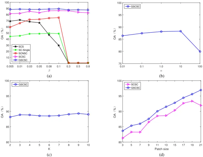
In the GSCSC model, there are tree key parameters: the sparsity regularization parameter β, the Laplacian constraint parameter α and K in KNN graph constraint. We test their influence to the classification performance on the Indian Pines dataset. The average results of five-runs on 10% randomly sampled training set are reported for all methods. Because only GSCSC has the Laplacian constraint parameterαandK
in KNN graph constraint, we analyse the influence ofαandK
to GSCSC only. The range of β is {0.005, 0.01, 0.03, 0.05, 0.08, 0.1, 0.3, 0.5, 0.8}. The range of α is {0.01, 0.1, 1.0, 10, 100} and the range of K is{2, 3, 4, 5, 6, 7, 8, 9, 10}, respectively.
The classification performance of different β values are shown in Fig. 6(a). The results show that models with no structural consistency are greatly influenced by the β value. Their performance fall abruptly when β is greater than 0.1. This is because the learned sparse coefficients will be too sparse and most entries are close to zero for SCS, SC-Single and SCNSC. SCS performs better when β is small.
0.005 0.01 0.03 0.05 0.08 0.1 0.3 0.5 0.8 β 10 20 30 40 50 60 70 80 90 100 SCS SC-Single SCNSC SCSC GSCSC 0.01 0.1 1.0 10 100 α 75 80 85 90 95 100 GSCSC (a) (b) 2 3 4 5 6 7 8 9 10 K 80 85 90 95 100 GSCSC 3 5 7 9 11 13 15 17 19 21 Patch size 80 85 90 95 100 SCSC GSCSC (c) (d)
Fig. 6. Classification performance under different (a)βvalues, (b)αvalues, (c)Kin KNN graph constraint, and (d) patch sizes.
10 20 30 40 50 60 70 80 90 100 110 120 130 140 150 160 170 180 190 200 Dictionary size 10 20 30 40 50 60 70 80 90 100 SCS SC-Single SCNSC SCSC GSCSC
Fig. 7. Classification performance under different dictionary sizes.
SC-Single and SCNSC work the best at 0.1. Models with structural consistency are much less influenced by small β. GSCSC changes more smoothly than SCSC. This implies that the graph regularized term smooths the model with spectral information and reduces the importance of the sparsity.
The classification performance of different α values are shown in Fig. 6(b). This figure shows that the performance of GSCSC decreases when α value is too large. In the
proposed model, α controls the contribution from the graph regularized term. When it is too large, the influence from structural consistency and sparsity are suppressed. Therefore, it is preferable to setαvalue between 1.0 and 10 for GSCSC. The classification performance of differentKin KNN graph constraint are shown in Fig. 6(c). GSCSC achieved very good performance with 3NN and 9NN, however, 3NN requires much less computation than 9NN. Therefore, in the rest of the experiments, we setK= 3.
D. Influence of patch size
It is well known that the patch size have an impact on clas-sification of HSI. We analyze the clasclas-sification performance with different patch sizes{3×3,5×5,7×7,9×9,11×11,13× 13,15×15,17×17,19×19,21×21}. Fig. 6(d) shows that the performance of both SCSC and GSCSC increases with larger patch size. However, the performance of SCSC starts to drop when the patch size reaches 21. This suggests that an appropriate patch size shall be set to obtain appropriate spatial distribution in a local neighborhood. For fair comparison with other methods, we follow the same setting in SOMP [44] and use 9×9 patch on the Indian Pines dataset and 5×5 patch on the University of Pavia dataset.
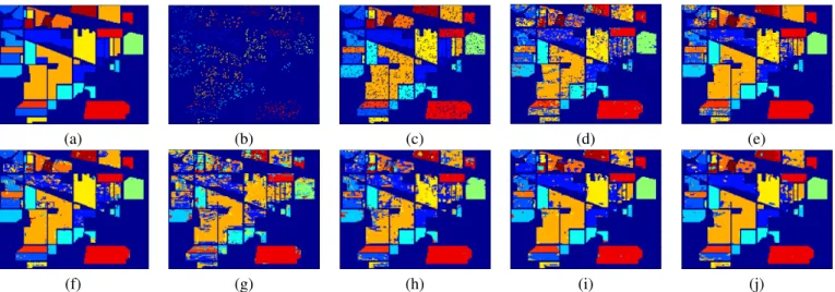
(a) (b) (c) (d) (e)
(f) (g) (h) (i) (j)
Fig. 8. Results on the Indian Pines dataset. (a) ground truth, (b) training set, and (c) testing set. Classification maps obtained by (d) SCS, (e) SOMP [44], (f) SWSC [48], (g) SC-Single, (h) SCNSC, (i) SCSC, and (j) GSCSC.
TABLE III
CLASSIFICATION ACCURACIES(%)ONINDIANPINES DATASET WITH10%LABELED SAMPLES USED FOR TRAINING. Class SCS SOMP [44] SWSC [48] SC-Single SCNSC SCSC GSCSC
1 80.49 75.61 95.12 43.90 85.37 85.37 90.24 2 65.29 73.46 88.72 42.65 70.82 84.67 84.12 3 51.94 59.04 95.45 20.48 68.14 83.40 85.27 4 31.46 59.15 75.12 12.68 53.05 52.58 75.12 5 81.61 94.02 93.33 67.82 83.22 94.94 96.09 6 88.89 97.56 95.59 58.14 94.52 96.35 98.78 7 80.00 44.00 96.00 20.00 32.00 68.00 80.00 8 93.26 100.00 97.21 53.26 92.09 99.30 100.00 9 11.11 22.22 55.56 44.44 27.78 38.89 38.89 10 61.94 60.34 92.91 9.94 60.57 79.66 79.66 11 74.06 93.03 68.99 69.71 73.83 86.69 88.82 12 41.01 58.24 87.45 9.18 49.81 74.91 76.59 13 75.00 92.93 99.46 65.76 100.00 95.65 99.46 14 95.87 99.91 96.84 89.10 95.96 97.80 97.63 15 44.09 81.27 88.76 34.29 60.23 70.32 77.23 16 91.67 98.81 98.81 11.90 35.71 79.76 94.05 OA 70.97 82.45 86.94 49.93 74.83 86.39 88.35 AA 66.73 75.60 89.08 40.83 67.69 80.52 85.12 κ 0.678 0.797 0.853 0.417 0.712 0.845 0.867
E. Influence of dictionary size
The sparse coding models are usually influenced easily by the dictionary size, so we look into this factor on the Indian pines dataset. We carry out the experiments with dictionary size {10, 20, 30, 40, 50, 60, 70, 80, 90, 100, 110, 120, 130, 140, 150, 160, 170, 180, 190, 200} and report the average results of five-runs with 10% randomly sampled training set. Other experimental setup is the same as that of Section IV-B. Fig. 7 shows the classification performance of the meth-ods with different dictionary sizes. Both SCSC and GSCSC achieve 85% accuracy when the dictionary size reaches 20, then their performance do not change much with larger dic-tionary. Figure 7 indicates that our methods can learn the dis-criminative sparse coefficients and achieve good performance with small dictionary size. SCSC and GSCSC obtain better results than SC-Single and SCNSC. This is because the pro-posed method explores structural consistency for better image description, but the alternatives do not have this property.
F. Results on the Indian Pines Dataset
On the Indian Pines dataset, we follow the same experiment settings to generate the training sets, the testing sets, and the patch size as SOMP [44]. Around 10% of the labeled samples are randomly chosen for training the classifier and the remaining are used for testing, as shown in Table I and Fig. 8(b) and (c) respectively. In the Indian Pines image, a large patch size 9×9 is used for all methods except for SCS. The Indian Pines image contains a lot of noises so that SCNSC gets very bad results in some bands when the sparse coefficients are calculated band by band separately. So we select some high quality bands to calculate the concatenated vectors of SCNSC, e.g., bands 6-52. For SC-Single, we use only the 30thband, which is a high quality band.
The classification results of the proposed methods and alter-natives are shown in Table III. It can be seen that SCSC and GSCSC, which use structural consistency in the modelling, have significantly improved the classification accuracy over the baseline sparse coding method SCS. SC-Single in one band generates very bad result. This is because SC-Single
(a) (b) (c) (d) (e)
(f) (g) (h) (i) (j)
Fig. 9. Results on the University of Pavia dataset. (a) ground truth, (b) training set, and (c) testing set. Classification maps obtained by (d) SCS, (e) SOMP [44], (f) SWSC [48], (g) SC-Single, (h) SCNSC, (i) SCSC, and (j) GSCSC
TABLE IV
CLASSIFICATION ACCURACIES(%)ONUNIVERSITY OFPAVIA DATASET WITH9%LABELED SAMPLES USED FOR TRAINING. Class SCS SOMP [44] SWSC [48] SC-Single SCNSC SCSC GSCSC
1 87.12 90.88 95.13 61.37 94.35 96.54 96.22 2 95.24 99.73 98.06 96.03 95.35 98.06 98.83 3 62.36 90.05 85.34 34.76 71.78 89.79 90.10 4 88.56 91.50 97.53 90.85 96.70 97.85 97.99 5 99.75 100.00 99.18 81.62 99.75 99.02 100.00 6 72.14 94.84 89.82 21.92 77.45 87.02 88.35 7 72.07 97.52 72.23 1.32 76.94 87.52 91.07 8 83.97 95.26 75.44 76.54 81.65 94.63 95.64 9 97.91 93.50 99.65 84.34 99.65 94.08 97.22 OA 87.68 96.16 93.29 73.24 90.51 95.42 96.19 AA 84.35 94.86 90.26 60.97 88.18 93.38 95.05 κ 0.836 0.949 0.911 0.627 0.874 0.939 0.949
only contains spatial information in a band and no any spectral information. SCNSC generates lower performance than SCSC and GSCSC since SCSC and GSCSC are benefit from struc-tural consistency. Raw image data may contain large amount of noises so that the structures in every band of image are less clear and the structures centered on some pixels are easily get mixed with noises. This makes SCNSC difficult to generate good performance. This result validates the effectiveness of our proposed methods with structural consistency. Moreover, GSCSC which is a model with the graph Laplacian sparsity constraints has shown better classification performance than the corresponding non-graph regularized SCSC. Compared with SOMP and SWSC, our method GSCSC has obtained better result.
The classification maps on labeled pixels are presented in Fig. 8(i) - (j). From this figure, we can see that the proposed
methods can effectively capture the inherent consistent struc-tures. Many pixels at the interior regions are misclassified by the SCS, SC-Single and SCNSC methods. On the contrary, most errors happen at the boundary regions in the results generated by SCSC and GSCSC methods. This implies that the local spatial structures are similar in different bands at the internal regions of every class. At the boundary pixels, the structure information of neighboring class may get involved, which causes the errors because the learned consistent struc-tures are easily confused between two neighboring classes. SOMP and SWSC with local spatial correlations also achieve better performance at big regions as shown in Fig. 8(e) and (f).
G. Results on the University of Pavia Dataset
We use the same experimental settings as in [44] to generate the training set, the testing set and the patch size on the University of Pavia dataset. Around9%of the labeled samples are randomly chosen for training and the remaining are used for testing. More detailed information on the training and testing sets are shown in Table II and Fig. 9(b) and (c). Considering the small spatial homogeneity in the University of Pavia image, a small patch size of5×5is used all methods except SCS. SCNSC uses all bands of sparse coefficients and concatenates them into a vector.
The classification results of various methods are presented in Table IV. Fig. 9(d) - (j) gives the classification maps on labeled pixels. The proposed methods achieve great improvement over the baseline SCS and are better than SC-Single and SCNSC with no structural consistency. They also generate slightly higher performance than SOMP and SWSC which are based on spatial correlations. From Fig. 9, we can see that the “Meadows” class at the bottom of the HSI is a large region and its internal pixels should have similar spatial structure and spectral information. Therefore, most pixels in this class are classified correctly by our methods. Because SCS captures only spectral information and SCNSC uses only spatial infor-mation, they are strongly influenced by the noises in different bands. The proposed methods explore spatial consistency and enforce the spatial structures along the spectral dimension, and thus show many advantages in the classification.
H. Performance under different training samples
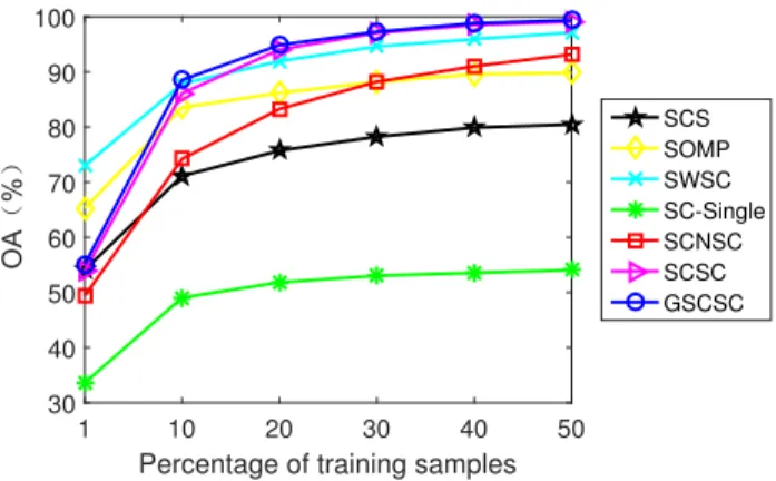
In this section, we analyze the classification performance of various methods with different sizes of training sets on the Indian pines dataset. we randomly select 1% to 50% from each class as the training sets and the rest samples are treated as the testing sets. Our evaluation measure is overall accuracy (OA) which is calculated from the mean of five-runs. When the number of training samples becomes large, the performance of all methods increases as shown in Fig. 10. The proposed methods have achieved great results and the performance of SCSC and GSCSC increases rapidly to above 95%. SOMP and SWSC incorporate spatial correlations between pixels and obtain good performance with a very small amount of training samples. SCSC and GSCSC surpass them as the training samples increase. The SC-Single’s accuracy is low under different training sizes because only one band of spatial patch is used. It does not capture sufficient spectral distribution of data. SCNSC outperforms SRS and SC-Single by exploring all bands for spatial information. SCSC and GSCSC enforce structural consistency on the model constantly and achieve better performance than SCNSC.
V. CONCLUSION
In this paper, we have introduced a novel joint spectral-spatial sparse coding model with structural consistency for HSI classification. This method captures the spatially consistent local structures in all bands by enforcing the same coefficient
1 10 20 30 40 50
Percentage of training samples
30 40 50 60 70 80 90 100 SCS SOMP SWSC SC-Single SCNSC SCSC GSCSC
Fig. 10. Classification performance under different training samples.
at the same location of different bands during the image recon-struction process. This model also preserves spectral charac-teristics of different bands by generating different dictionaries. A graph Laplacian sparsity constraints is combined into the proposed method to make the learned sparse coefficients better characterize the relationships between spectral responses. We have validated the effectiveness of the proposed methods on two real-world HSI datasets. The experimental results show that our methods significantly outperform the baseline approach. The proposed method is general in nature and can incorporate other 2D spatial features for HSI classification. We will explore this direction in the future work.
REFERENCES
[1] D. A. Landgrebe,Signal theory methods in multispectral remote sensing. Hoboken, NJ: Wiley, 2003.
[2] J. Ham, Y. Chen, M. M. Crawford, and J. Ghosh, “Investigation of the random forest framework for classification of hyperspectral data,”IEEE Trans. Geosci. Remote Sens., vol. 43, no. 3, pp. 492–501, 2005. [3] F. R. Ratle, G. Camps-Valls, and J. Weston, “Semisupervised neural
networks for efficient hyperspectral image classification,”IEEE Trans. Geosci. Remote Sens., vol. 48, no. 5, pp. 2271–2282, 2010.
[4] F. Melgani and L. Bruzzone, “Classification of hyperspectral remote sensing images with support vector machines,” IEEE Trans. Geosci. Remote Sens., vol. 42, no. 8, pp. 1778–1790, 2004.
[5] M. Fauvel, J. Chanussot, and J. A. Benediktsson, “Evaluation of kernels for multiclass classification of hyperspectral remote sensing data,” in
Proc. IEEE Conference on Acoustics Speech and Signal Processing (ICASSP’06), 2006, pp. 813–816.
[6] L. Gao, J. Li, M. Khodadadzadeh, A. J. Plaza, B. Zhang, Z. He, and H. Yan, “Subspace-based support vector machines for hyperspectral image classification,”IEEE Geosci. Remote Sens. Lett., vol. 12, no. 2, pp. 349–353, 2015.
[7] J. Peng, Y. Zhou, and C. L. P. Chen, “Region-kernel-based support vector machines for hyperspectral image classification,” IEEE Trans. Geosci. Remote Sens., vol. 53, no. 9, pp. 4810–4824, 2015.
[8] Y. Chen, N. M. Nasrabadi, and T. D. Tran, “Sparsity-based classification of hyperspectral imagery,” in Proc. IEEE Geoscience and Remote Sensing Symposium (IGARSS’10), 2010, pp. 2796–2799.
[9] A. S. Charles, B. A. Olshausen, and C. J. Rozell, “Learning sparse codes for hyperspectral imagery,”J. Sel. Topics Signal Processing, vol. 5, no. 5, pp. 963–978, 2011.
[10] Y. Chen, N. M. Nasrabadi, and T. D. Tran, “Hyperspectral image classification via kernel sparse representation,” IEEE Trans. Geosci. Remote Sens., vol. 51, no. 1, pp. 217–231, 2013.
[11] J.-H. Yang, L.-G. Wang, and J.-X. Qian, “Hyperspectral image classifi-cation based on spatial and spectral features and sparse representation,”
Applied Geophysics, vol. 11, no. 4, pp. 489–499, 2014.
[12] X. Sun, Q. Qu, N. M. Nasrabadi, and T. D. Tran, “Structured priors for sparse-representation-based hyperspectral image classification,” IEEE Geosci. Remote Sens. Lett., vol. 11, no. 7, pp. 1235–1239, 2014.
[13] L. He, Y. Li, X. Li, and W. Wu, “Spectral-spatial classification of hy-perspectral images via spatial translation-invariant wavelet-based sparse representation,”IEEE Trans. Geosci. Remote Sens., vol. 53, no. 5, pp. 2696–2712, 2015.
[14] M. E. Midhun, S. R. Nair, V. T. N. Prabhakar, and S. S. Kumar, “Deep model for classification of hyperspectral image using restricted Boltz-mann machine,” inProc. International Conference on Interdisciplinary Advances in Applied Computing, 2014, pp. 1–7.
[15] Y. Chen, X. Zhao, and X. Jia, “Spectralcspatial classification of hyper-spectral data based on deep belief network,”IEEE J. Sel. Topics Appl. Earth Observ. Remote Sens., vol. 8, no. 6, pp. 2381–2392, 2015. [16] A. Plaza, J. A. Benediktsson, J. W. Boardman, J. Brazile, L. Bruzzone,
G. Camps-Valls, J. Chanussot, M. Fauvel, P. Gamba, A. Gualtieri, M. Marconcini, J. C. Tilton, and G. Trianni, “Recent advances in techniques for hyperspectral image processing,” Remote Sensing of Environment, vol. 113, no. 9, pp. S110–S122, 2009.
[17] U. Srinivas, Y. Chen, V. Monga, N. M. Nasrabadi, and T. D. Tran, “Exploiting sparsity in hyperspectral image classification via graphical models,”IEEE Geosci. Remote Sensing Lett., vol. 10, no. 3, pp. 505– 509, 2013.
[18] Z. tao Qin, W. nian Yang, R. Yang, X. yu Zhao, and T. jiao Yang, “Dictionary-based, clustered sparse representation for hyperspectral im-age classification,”Journal of Spectroscopy, 2015.
[19] W. Li, Q. Du, F. Zhang, and W. Hu, “Hyperspectral image classification by fusing collaborative and sparse representations,”IEEE J. Sel. Topics Appl. Earth Observ. Remote Sens., vol. PP, no. 99, pp. 1–20, 2016. [20] M. Fauvel, Y. Tarabalka, J. A. Benediktsson, J. Chanussot, and J. C.
Tilton, “Advances in spectral-spatial classification of hyperspectral im-ages,”Proceedings of the IEEE, vol. 101, no. 3, pp. 652–675, 2013. [21] Z. H. Nezhad, A. Karami, R. Heylen, and P. Scheunders, “Fusion of
hyperspectral and multispectral images using spectral unmixing and sparse coding,”IEEE J. Sel. Topics Appl. Earth Observ. Remote Sens., vol. 9, no. 6, pp. 2377–2389, 2016.
[22] M. D. Mura, A. Villa, J. A. Benediktsson, J. Chanussot, and L. Bruzzone, “Classification of hyperspectral images by using extended morphological attribute profiles and independent component analysis,”IEEE Geosci. Remote Sens. Lett., vol. 8, no. 3, pp. 542–546, 2011.
[23] P. Ghamisi, M. D. Mura, and J. A. Benediktsson, “A survey on spectral-spatial classification techniques based on attribute profiles,”IEEE Trans. Geosci. Remote Sens., vol. 53, no. 5, pp. 2335–2353, 2015.
[24] X. Jia and J. Richards, “Managing the spectral-spatial mix in context classification using Markov random fields,”IEEE Geosci. Remote Sens. Lett., vol. 5, pp. 311–314, 2008.
[25] J. Xia, J. Chanussot, P. Du, and X. He, “Spectral-spatial classification for hyperspectral data using rotation forests with local feature extraction and Markov random fields,”IEEE Trans. Geosci. Remote Sens., vol. 53, no. 5, pp. 2532–2546, 2015.
[26] Y. Qian, M. Ye, and J. Zhou, “Hyperspectral image classification based on structured sparse logistic regression and three-dimensional wavelet texture features,”IEEE Trans. Geosci. Remote Sens., vol. 51, no. 4-2, pp. 2276–2291, 2013.
[27] J. Liu, Z. Wu, Z. Wei, L. Xiao, and L. Sun, “Spatial-spectral kernel sparse representation for hyperspectral image classification,”IEEE J. Sel. Topics Appl. Earth Observ. Remote Sens., vol. 6, no. 6, pp. 2462– 2471, Dec 2013.
[28] Z. He, Q. Wang, Y. Shen, and M. Sun, “Kernel sparse multitask learning for hyperspectral image classification with empirical mode decomposition and morphological wavelet-based features,”IEEE Trans. Geosci. Remote Sens., vol. 52, no. 8, pp. 5150–5163, 2014.
[29] H. Zhang, J. Li, Y. Huang, and L. Zhang, “A nonlocal weighted joint sparse representation classification method for hyperspectral imagery,”
IEEE J. Sel. Topics Appl. Earth Observ. Remote Sens., vol. 7, no. 6, pp. 2056–2065, 2014.
[30] J. Wang, L. Jiao, H. Liu, S. Yang, and F. Liu, “Hyperspectral image classification by spatialcspectral derivative-aided kernel joint sparse representation,”IEEE J. Sel. Topics Appl. Earth Observ. Remote Sens., vol. 8, no. 6, pp. 2485–2500, June 2015.
[31] S. Jia, J. Hu, Y. Xie, L. Shen, X. Jia, and Q. Li, “Gabor cube selection based multitask joint sparse representation for hyperspectral image classification,”IEEE Trans. Geosci. Remote Sens., vol. 54, no. 6, pp. 3174–3187, 2016.
[32] Z. Xue, P. Du, J. Li, and H. Su, “Simultaneous sparse graph embedding for hyperspectral image classification,” IEEE Trans. Geosci. Remote Sens., vol. 53, no. 11, pp. 6114–6133, 2015.
[33] J. Wright, A. Y. Yang, A. Ganesh, S. S. Sastry, and Y. Ma, “Robust face recognition via sparse representation,”IEEE Trans. Pattern Anal. Mach. Intell., vol. 31, no. 2, pp. 210–227, 2009.
[34] J. Wright, Y. Ma, J. Mairal, G. Sapiro, T. S. Huang, and S. Yan, “Sparse representation for computer vision and pattern recognition,”Proceedings of the IEEE, vol. 98, no. 6, pp. 1031–1044, 2010.
[35] Z. Shu, J. Zhou, P. Huang, X. Yu, Z. Yang, and C. Zhao, “Local and global regularized sparse coding for data representation,” Neurocomput-ing, vol. 175, pp. 188–197, 2016.
[36] M. Zheng, J. Bu, C. Chen, C. Wang, L. Zhang, G. Qiu, and D. Cai, “Graph regularized sparse coding for image representation,”IEEE Trans. Image Process., vol. 20, no. 5, pp. 1327–1336, 2011.
[37] S. Gao, I. W.-H. Tsang, and L.-T. Chia, “Laplacian sparse coding, hypergraph laplacian sparse coding, and applications,” IEEE Trans. Pattern Anal. Mach. Intell., vol. 35, no. 1, pp. 92–104, 2013. [38] L. Tong, J. Zhou, X. Bai, and Y. Gao, “Dual graph regularized NMF for
hyperspectral unmixing,” inProc. International Conference on Digital Image Computing: Techniques and Applications, 2014, pp. 1–8. [39] Z. Shu, J. Zhou, L. Tong, X. Bai, and C. Zhao, “Multilayer manifold and
sparsity constrainted nonnegative matrix factorization for hyperspectral unmixing,” inProc. IEEE Conference on Image Processing (ICIP’15), 2015, pp. 2174–2178.
[40] E. Berg and M. P. Friedlander, “Joint-sparse recovery from multiple measurements,”IEEE Trans. Inf. Theory, vol. 56, no. 5, pp. 2516–2527, 2010.
[41] A. Rakotomamonjy, “Surveying and comparing simultaneous sparse approximation (or group-lasso) algorithms,”Signal Processing, vol. 91, no. 7, pp. 1505–1526, 2011.
[42] G. Liu, Z. Lin, S. Yan, J. Sun, Y. Yu, and Y. Ma, “Robust recovery of subspace structures by low-rank representation,”IEEE Trans. Pattern Anal. Mach. Intell., vol. 35, no. 1, pp. 171–184, 2013.
[43] M. Ye, Y. Qian, and J. Zhou, “Multitask sparse nonnegative matrix factorization for joint spectral-spatial hyperspectral imagery denoising,”
IEEE Trans. Geosci. Remote Sens., vol. 53, no. 5, pp. 2621–2639, 2015. [44] Y. Chen, N. M. Nasrabadi, and T. D. Tran, “Hyperspectral image classification using dictionary-based sparse representation,”IEEE Trans. Geosci. Remote Sens., vol. 49, no. 10, pp. 3973–3985, 2011. [45] S. Jia, X. Zhang, and Q. Li, “Spectralspatial hyperspectral image
classification using`1/2regularized low-rank representation and sparse representation-based graph cuts,” IEEE J. Sel. Topics Appl. Earth Observ. Remote Sens., vol. 8, no. 6, pp. 2473–2484, 2015.
[46] H. Yuan and Y. Y. Tang, “Sparse representation based on set-to-set distance for hyperspectral image classification,”IEEE J. Sel. Topics Appl. Earth Observ. Remote Sens., vol. 8, no. 6, pp. 2464–2472, 2015. [47] E. Zhang, L. Jiao, X. Zhang, H. Liu, and S. Wang, “Class-level
joint sparse representation for multifeature-based hyperspectral image classification,”IEEE J. Sel. Topics Appl. Earth Observ. Remote Sens., vol. PP, no. 99, pp. 1–18, 2016.
[48] A. S. Farani and H. R. Rabiee, “When pixels team up: Spatially weighted sparse coding for hyperspectral image classification,” IEEE Geosci. Remote Sens. Lett., vol. 12, no. 1, pp. 107–111, 2015.
[49] H. Lee, A. Battle, R. Raina, and A. Y. Ng, “Efficient sparse coding al-gorithms,” inProc. Advances in Neural Information Processing Systems (NIPS’06), 2006, pp. 801–808.
[50] R. Fletcher,Practical methods of optimization. Hoboken, NJ: Wiley, 1987.
[51] VIRIS NW Indianas Indian Pines 1992 data set. [Online]. Available: http://cobweb.ecn.purdue.edu/biehl/MultiSpec/documentation.html [52] C.-C. Chang and C.-J. Lin, “LIBSVM: A library for support vector
machines,”ACM Transactions on Intelligent Systems and Technology, vol. 2, no. 3, pp. 389–396, 2011.
[53] J. A. Richards,Remote Sensing Digital Image Analysis: An Introduction, 5th ed. New York, NY, USA: Springer Berlin Heidelberg, 2013.
Changhong Liureceived the B.S. and M.S. degrees in computer science from Jiangxi Normal University, Nanchang, China, in 2000 and 2004, respectively, and the Ph.D. degree in computer application tech-nology from University of Science& Technology Beijing, Beijing, China, in 2011.
She is currently a lecturer in the School of Com-puter and Information Engineering, Jiangxi Normal University, China. During 2015, she was a Visiting Fellow in the School of Information and Commu-nication Technology at Griffith University, Nathan, Australia. Her research interests include pattern recognition, hyperspectral imaging, computer vision, and machine learning.
Jun Zhou received the B.S. degree in computer science and the B.E. degree in international business from Nanjing University of Science and Technology, Nanjing, China, in 1996 and 1998, respectively. He received the M.S. degree in computer science from Concordia University, Montreal, Canada, in 2002, and the Ph.D. degree from the University of Alberta, Edmonton, Canada, in 2006.
He is a senior lecturer in the School of Infor-mation and Communication Technology at Griffith University, Nathan, Australia. Previously, he had been a research fellow in the Research School of Computer Science at the Australian National University, Canberra, Australia, and a researcher in the Canberra Research Laboratory, NICTA, Australia. His research interests include pattern recognition, computer vision and spectral imaging with their applications to remote sensing and environmental informatics.
Jie Liang Jie Liang received the B.E. degree in automatic control from National University of De-fense Technology, Changsha, China, in 2011. He is currently working toward the Ph.D. degree in the Research School of Engineering, Australian National University, Canberra, Australia. He is also a visiting scholar in the School of Information of Commu-nication Technology at Griffith University, Nathan, Australia.
His research topic is spectral-spatial feature ex-traction for hyperspectral image classification.
Yuntao Qian (M’04) received the B.E. and M.E. degrees in automatic control from Xi’an Jiaotong University, Xi’an, China, in 1989 and 1992, respec-tively, and the Ph.D. degree in signal processing from Xidian University, Xi’an, China, in 1996.
During 1996–1998, he was a Postdoctoral Fel-low with the Northwestern Polytechnical University, Xi’an, China. Since 1998, he has been with the College of Computer Science, Zhejiang University, Hangzhou, China, where he is currently a Profes-sor in computer science. During 1999–2001, 2006, 2010, and 2013, he was a Visiting Professor at Concordia University, Hong Kong Baptist University, Carnegie Mellon University, the Canberra Research Laboratory of NICTA, and Griffith University. His current research interests include machine learning, signal and image processing, pattern recognition, and hyperspectral imaging.
Prof. Qian is an Associate Editor of the IEEE JOURNAL OFSELECTED
TOPICS INAPPLIEDEARTHOBSERVATIONS ANDREMOTESENSING
Hanxi Lireceived the B.Sc. and M.Sc. degrees from the School of Automation Science and Electrical Engineering, Beihang University, Beijing, China, in 2004 and 2007 respectively, and the Ph.D. degree from the Research School of Information Science and Engineering at the Australian National Univer-sity, Canberra, Australia, in 2011.
He was a Researcher at NICTA (Australia) from 2011-2015. He is currently a Special Term Pro-fessor in the School of Computer and Information Engineering, Jiangxi Normal University, China. His recent areas of interest include visual tracking, face recognition, and deep learning.
Yongsheng Gaoreceived the B.Sc. and M.Sc. de-grees in electronic engineering from Zhejiang Uni-versity, Hangzhou, China, in 1985 and 1988, respec-tively, and the Ph.D. degree in computer engineering from Nanyang Technological University, Singapore. He is currently a Professor with the School of En-gineering, Griffith University, Brisbane, QLD, Aus-tralia. He had been the Leader of Biosecurity Group, Queensland Research Laboratory, National ICT Aus-tralia (ARC Centre of Excellence), a consultant of Panasonic Singapore Laboratories, and an Assistant Professor in the School of Computer Engineering, Nanyang Technological University, Singapore.
His research interests include face recognition, biometrics, biosecurity, im-age retrieval, computer vision, pattern recognition, environmental informatics, and medical imaging.