lordif: An R Package for Detecting Differential Item Functioning Using Iterative Hybrid Ordinal Logistic Regression/Item Response Theory and Monte Carlo Simulations

March 2011, Volume 39, Issue 8. http://www.jstatsoft.org/

lordif

: An

R

Package for Detecting Differential Item

Functioning Using Iterative Hybrid Ordinal Logistic

Regression/Item Response Theory and Monte

Carlo Simulations

Logistic regression provides a flexible framework for detecting various types of dif-ferential item functioning (DIF). Previous efforts extended the framework by using item response theory (IRT) based trait scores, and by employing an iterative process using group–specific item parameters to account for DIF in the trait scores, analogous to pu-rification approaches used in other DIF detection frameworks. The current investigation advances the technique by developing a computational platform integrating both statis-tical and IRT procedures into a single program. Furthermore, a Monte Carlo simulation approach was incorporated to derive empirical criteria for various DIF statistics and ef-fect size measures. For purposes of illustration, the procedure was applied to data from a questionnaire of anxiety symptoms for detecting DIF associated with age from the Patient–Reported Outcomes Measurement Information System.

Keywords: DIF, ordinal logistic regression, IRT, R.

1. Introduction

Standardized tests and questionnaires are used in many settings, including education, psy-chology, business, and medicine. Investigations across numerous disciplines have identified respondent culture (more generally, any group membership irrelevant of the construct being measured) as a potential source of systematic measurement variability in survey research ( An-dersen 1967). Systematic measurement variability can lead to a number of problems including errors in hypothesis testing, flawed population forecasts, policy planning and implementation, and misguided research on disparities (Perkinset al.2006). Ensuring equivalent measurement

is important prior to making comparisons among individuals or groups (Gregorich 2006). Evaluations of item-level measurement equivalence have come to focus on DIF, defined as different probabilities of success or endorsement across construct-irrelevant groups when con-trolling for the underlying trait measured by the test (Camilli and Shepard 1994). There are many other frameworks for DIF detection, including explanatory item response model formulation (De Boeck and Wilson 2004), the multiple indicators multiple causes (MIMIC) formulation (Jones 2006), and the SIBTEST framework (Shealy and Stout 1993). This paper addresses the logistic regression framework, which provides a flexible model-based framework for detecting various types of DIF (Swaminathan and Rogers 1990;Zumbo 1999).

Previous efforts extended the logistic regression DIF technique into a framework known as difwithpar (Craneet al.2006) by using IRT based trait estimates and employing an iterative process of accounting for DIF in the trait estimate with the use of group-specific IRT item parameters for items identified with DIF (Craneet al. 2006,2007b,c,2004). This framework has been found to be facile at accounting for multiple sources of DIF and paying specific attention to DIF impact. It is also able to address covariates with more than two categories, rather than limiting to only focal and reference groups.

Thedifwithpar software includes user-specified flagging criteria (or detection thresholds) for identifying items with DIF, and the developers have investigated the implications of different choices for these flagging criteria (Craneet al.2007c). Several values may be used for flagging criteria in analyzing a single dataset, resulting in varying numbers of items identified with DIF, but fairly consistent DIF impact for individuals and groups across different values for the flagging criteria (Crane et al.2007b). These observations suggest the need for empirical identification of flagging criteria.

To date, while the difwithpar software is freely distributed on the web (type ssc install

difwithparat theStataprompt), it uses the proprietary software packagesStata(StataCorp.

2007) and PARSCALE (Muraki and Bock 2005). Recent developments of free IRT packages forR(RDevelopment Core Team 2010), such aseRm(Mair and Hatzinger 2007) and especially the IRT/latent trait modeling package ltm (Rizopoulos 2006), suggested the possibility of integrating the framework in a freeware platform. The current investigation advances the difwithpar technique by creating a computational platform integrating both statistical and IRT procedures into a single freeware program. Furthermore, we provide a mechanism to evaluate statistical criteria proposed for detecting DIF using graphical approaches and Monte Carlo simulations. The resulting R package lordif is available from the Comprehensive R Archive Network athttp://CRAN.R-project.org/package=lordif.

2. Logistic regression/IRT hybrid DIF detection method

Swaminathan and Rogers(1990) proposed the use of logistic regression in DIF detection for dichotomous items. Several researchers have extended the technique for polytomous items (French and Miller 1996; Miller and Spray 1993; Zumbo 1999). For polytomous items, the proportional-odds logistic regression model (Agresti 1990) is used with the assumption that the outcome variable is ordinal (as opposed to nominal). Let Ui denote a discrete random variable representing the ordered item response to itemi, andui (= 0,1, . . . , mi−1) denote

the actual response to itemiwithmi ordered response categories. Based on the proportional odds assumption or the parallel regression assumption, a single set of regression coefficients is estimated for all cumulative logits with varying intercepts (αk). For each item, an intercept-only (null) model and three nested models are formed in hierarchy with additional explanatory variables as follows:

Model 0 : logitP(ui≥k) =αk

Model 1 : logitP(ui≥k) =αk+β1∗ability

Model 2 : logitP(ui≥k) =αk+β1∗ability +β2∗group

Model 3 : logitP(ui≥k) =αk+β1∗ability +β2∗group +β2∗ability∗group, whereP(ui≥k) denotes the cumulative probabilities that the actual item responseui falls in category kor higher. The term “ability” is used broadly here to represent the trait measured by the test as either the observed sum score or a latent variable. Without loss of generality the term “trait level” may be substituted in each case. In the remainder of this paper, we use these terms somewhat interchangeably.

2.2. DIF detection

Testing for the presence of DIF (both uniform and non-uniform) under the logistic regression framework is traditionally based on the likelihood ratio χ2 test (Swaminathan and Rogers 1990). DIF is classified as either uniform (if the effect is constant) or non-uniform (if the effect varies conditional on the trait level). Uniform DIF may be tested by comparing the log likelihood values for Models 1 and 2 (one degree of freedom, ordf = 1), and non-uniform DIF by Models 2 and 3 (df = 1). An overall test of “total DIF effect” is tenable by comparing Models 1 and 3 (df = 2). The 2-df χ2 test was designed to maximize the ability of this procedure to identify both uniform and non-uniform DIF and control the overall Type I error rate. However, the component uniquely attributable to either uniform or non-uniform DIF can be partitioned separately by the 1-df tests (Jodoin and Gierl 2001;Zumbo 1999). The extension of this framework for multiple groups is also straightforward. Theβ2 and β3 terms from Models 2 and 3 are expanded to include binary indicator variables for all of the groups except one. For both uniform (Model 1 vs. 2) and non-uniform DIF (Model 2 vs. 3) twice the difference in log likelihoods is compared to aχ2 distribution with degrees of freedom equal to the number of groups minus one.

2.3. DIF magnitude

Although the likelihood ratio test has been found to yield good Type I error control (Kim and Cohen 1998), some researchers have reported good power but inflated Type I error under the logistic regression likelihood ratio test (Li and Stout 1996; Rogers and Swaminathan 1993;Swaminathan and Rogers 1990). Because statistical power is dependent on sample size (Cohen 1988), a trivial but non-zero difference in population parameters will be found to be statistically significant given a large enough sample. In response to this concern, several effect size measures have been used to quantify the magnitude of DIF (Crane et al. 2004; Jodoin and Gierl 2001; Kim et al. 2007; Zumbo 1999). Zumbo (1999) suggested several pseudo R2

statistics as magnitude measures and guidelines for classifying DIF as negligible (< 0.13), moderate (between 0.13 and 0.26), and large (>0.26). Subsequent studies (Jodoin and Gierl

2001; Kim et al. 2007), however, found the proposed thresholds to be too large, resulting in under-identification of DIF. Kim et al. (2007) also found that the pseudo R2 measures are closely related (with almost perfect rank order correlations) to some standardized impact indices (Wainer 1993).

Jodoin and Gierl (2001) noted that the regression coefficients β2 and β3 can be used as magnitude measures of uniform and non-uniform DIF, respectively. The difference in the β1 coefficient from Models 1 and 2 has also been used to identify items with uniform DIF (Crane et al. 2004). Based on simulation studies in a different context (Maldonado and Greenland 1993), 10% differences in this coefficient from Models 1 and 2 was initially proposed as a practically meaningful effect (Crane et al. 2004). Subsequent studies used lower thresholds such as 5% and even 1% (Crane et al.2007c).

2.4. Monte Carlo simulation approach to determining detection thresholds

Within the logistic regression DIF detection framework, there is considerable variability in specific criteria recommended for determining whether items exhibit DIF. Several experts have recommended magnitude measures with a plea towards “clinical relevance,” though specific thresholds based on this plea are not clearly discernible. Some authors have recommended a flexible, almost analog procedure in which the threshold used for a given parameter to identify items with and without DIF is manipulated up and down, and the effect on DIF impact for individuals or groups is evaluated (Craneet al. 2007c,a,2010,2008b,a;Gibbonset al.2009). Given the variety of DIF magnitude measures and detection criteria, a Monte Carlo simu-lation approach may be useful. Two general approaches are feasible, one driven by Type I error and another by Type II error. The Type I error approach involves generating multiple datasets (of the same dimension as the real data) under the null hypothesis (i.e., no DIF), preserving observed group differences in ability (trait level). Various magnitude measures are computed repeatedly over the simulated datasets, from which the empirical distributions are obtained. The researcher can then be guided by these empirical distributions when making a determination with any particular magnitude measure whether items have DIF. The target threshold to use in the real data is one where the empirical probability of identifying an item as displaying DIF (i.e., false positives) is not greater than the preset nominalα level. The Type II error approach, which is not implemented in lordif for the reasons provided below, involves generating multiple datasets as before, preserving group differences. However, the Type II error approach also involves introducing known DIF of varying magnitude, deemed as minimally detectable (e.g., power ≥0.80), to a varying number of items. Again, the mag-nitude measures are computed over the simulated datasets and their empirical distributions are obtained. Reviewing the empirical distributions the researcher can determine a target threshold to use in the real data. Unlike in the Type I error approach, the target threshold corresponds to a typical value in the empirical distribution (e.g., the median) rather than an extreme one that cuts off the tail end of the distribution. The choice of the magnitude of DIF introduced and the specific items having DIF can affect the simulation outcome (Donoghue et al.1993) and hence makes it difficult to implement the Type II error approach in a general simulation framework.

2.5. Iterative purification of the matching criterion

the trait being measured. The matching criterion, the variable by which the respondents are matched, is important in order to distinguish between differences in item functioning from differences between groups (Dorans and Holland 1993). One of the potential limitations of logistic regression DIF detection was the reliance on the observed sum score as the matching criterion. AsMillsap and Everson(1993) point out, the sum score is not a very good matching criterion unless statistical properties of the Rasch model hold (e.g., equal discrimination power for all items). Even if the Rasch model holds, using the sum score in a regression framework may not be ideal because the relationship between the sum score and the Rasch trait score is not linear, as evident in a test characteristic curve. In such situations, an IRT trait score is a more reasonable choice for regression modeling (such as DIF detection in the ordinal logistic regression framework) than an observed sum score (Craneet al. 2008a).

Another consideration for obtaining the matching criterion is related to purification. Zumbo (1999) advocated purifying the matching criterion by recalculating it using only the items that are identified as not having DIF. French and Maller (2007) reported that purification was beneficial under certain conditions, although overall power and Type I error rates did not substantially improve. Holland and Thayer(1988) suggested that the item under examination should be included in the matching criterion even if it was identified as having DIF but excluded from the criterion for all other items to reduce the Type I error rate. Zwick (1990) also proved theoretically that excluding the studied item from the matching variable leads to a bias (over detection) under the null condition.

Eliminating items found to have DIF is only one option for reducing the effect of DIF on the trait estimates used for the matching criterion. Reiseet al.(1993) pointed out that although items with DIF measure differently in different groups, they are still measuring the same underlying construct. This point is especially relevant in psychological measures where some items can be considered crucial in measuring a certain construct (e.g., crying in measuring depression), even if they are known to function differently between some demographic groups (e.g., gender).

To address these issues, Crane et al. (2006) developed an iterative process to update trait estimates using group-specific IRT item parameter estimates for items found to have DIF. Specifically, each item with DIF is replaced by as many sparse items (response vectors) as there are groups. For example, if there are two groups, A and B, two new sparse item response vectors are formed to replace the original. In the first sparse item response vector, the responses are the same as the original item for group A, and missing for group B. In the second sparse item response vector, the pattern is reversed.

The non-DIF items have parameters estimated using data from the entire sample and are often referred to as anchor items because they ensure that scores for individuals in all of the groups are on the same metric. The group-specific items and the anchor items are used to obtain trait estimates that account for DIF which in turn are then used in subsequent logistic regression DIF analyses. This process is continued until the same set of items is found to have DIF over successive iterations.

This algorithm has much to recommend it compared with more traditional purification ap-proaches. First, it is possible for items to have false positive identification with DIF at an early stage. Most traditional purification approaches would result in such an item being ex-cluded from consideration for the matching criterion, even though in the subsequent iterations it may be found to not have DIF. Second, by including all of the items in the trait estimate,

the measurement precision using this approach will be better than that for trait estimates that includes only a subset of the items. Finally, the iterative nature of this procedure avoids the forward stepwise nature of some algorithms, such as that used in the multiple indicators multiple causes framework (Jones 2006).

2.6. Fitting the graded response model

Unlike other IRT-based DIF detection methods focusing on tests of the equality of item parameters across groups (Lord 1980;Raju et al. 2009;Thissen 2001), the main objective of fitting an IRT model under lordif is to obtain IRT trait estimates to serve as the matching criterion. Therefore, the choice of a specific IRT model is of little consequence in the current application, because trait estimates for the same data based on different IRT models (e.g., graded response model vs. Generalized Partial Credit Model) are virtually interchangeable (r > 0.99) (Cook 1999). However, the graded response model might be preferred in the current context on the basis of its inherent connection to ordinal logistic regression. The model assumes any response to item i, ui, can be scored into mi ordered categories, e.g.,

ui ∈ {0,1,2, . . . ,(mi −1)}. The model then defines (mi −1) cumulative category response functions as follows: P₁∗(θ)≡P(ui≥1|θ) ={1 +exp[−ai(θ−bi1)]} −1 P₂∗(θ)≡P(ui≥2|θ) ={1 +exp[−ai(θ−bi2)]} −1 . . . P₍∗_m i−1)(θ)≡P(ui ≥mi−1|θ) ={1 +exp[−ai(θ−bi(_mi−1))]} −1

where the item discrimination parameteraiis finite and positive, and the location parameters,

bi1, bi2, . . . , bi(_mi−1), satisfy

bi1 < bi2 < . . . < bi(_mi−1).

Further, bi0 ≡ −∞and bi_mi ≡ ∞such that P

∗

0 = 1 and P(∗mi) = 0. Finally, for any response

category, ui ∈ {0,1, . . . , mi−1}, the category response function can be expressed as

Pui(θ) =P ∗ ui(θ)−P ∗ (ui+1)(θ)>0. 2.7. Scale transformation

The impact of DIF on scores can be determined by comparing the initial trait score to the final trait score that accounts for DIF. To compare scores, however, the IRT item parameter estimates from the initial and final calibrations should be placed on the same metric. The method developed by Stocking and Lord (1983) can be used to determine the appropriate transformation. Using the non-DIF items as anchor items, the procedure can equate the group-specific item parameter estimates from the final “matrix” calibration (M) to the metric of the initial “single-group” calibration (S). The Stocking-Lord equating procedure finds the linear transformation constants, A and B, that minimize the sum of squared differences between the test characteristic curves (T CCs) based on J non-DIF items over aθ grid (e.g., −4≤θ≤4). The loss function (L) to be minimized can be expressed as follows:

L= Q X

q=1

T CCS(θq) = J X i=1 X k∈ui k·P(ui=k|θq, aiS, bi1_S, bi2_S, . . . , bi(_mi−1)_S), T CCM(θq) = J X i=1 X k∈ui k·P(ui=k|θq, a∗iM, b ∗ i1_M, b ∗ i2_M, . . . , b ∗ i(_mi−1)_M), a∗_iM = aiM A , b∗_i1 M =A·bi1M +B, b∗_i2 M =A·bi2M +B, . . . b∗_i( mi−1)_M =A·bi(_mi−1)_M +B,

where Q is the number of equi-spaced quadrature points over the θ grid, J is the number of non-DIF items, aiS, bi1_S, bi2_S, . . . , bi(_mi−1)_S are the single-group item parameter estimates

for the ith non-DIF item, and a∗_iM, b∗_i1

M, b

∗

i2_M, . . . , bi(_mi−1)_M are the matrix calibration item

parameter estimates for the same item.

3. The

lordif

package

The lordif package is based on the difwithpar framework (Craneet al.2006). We developed the lordif package (available from the Comprehensive R Archive Network at http://CRAN. R-project.org/package=lordif) to perform DIF detection with a flexible iterative hybrid OLR/IRT framework. The lordif package is also able to perform OLR with sum scores rather than IRT scores. lordifalso incorporates a Monte Carlo simulation approach to derive empirical threshold values for various DIF statistics and magnitude measures. The lordif package generates DIF-free datasets of the same dimension as the empirical dataset using the purified trait estimates and initial single-group item parameter estimates obtained from the real data, preserving observed group differences and distributions. The user specifies the number of replications (nr) and the Type I error rate (e.g., alpha = 0.01). The program then applies the OLR/IRT procedure over the simulated DIF-free datasets and computes the statistics and magnitude measures. Finally, the program identifies a threshold value that cuts off the most extreme (α×100)% of each of the statistics and magnitude measures.

Thelordifpackage is built on two main packages: Theltmpackage (Rizopoulos 2006) to obtain IRT item parameter estimates according to the graded response model (Samejima 1969) and the Design package (Harrell Jr. 2009) for fitting (ordinal) logistic regression models. Both theltmandDesign packages can handle binary outcome variables as a special case and hence allow the lordif package to handle both dichotomous and polytomous items. The Design package also handles a grouping variable with more than two levels (e.g., Black, Hispanic and White) by automatically entering it into a model as a set of dummy variables.

The lordif package allows the user to choose specific criteria and their associated thresholds for declaring items to have uniform and non-uniform DIF. Items found displaying DIF are recalibrated in appropriate subgroups to generate trait estimates that account for DIF. These steps are repeated until the same items are identified with DIF on consecutive runs. The program uses the Stocking and Lord (1983) equating procedure to place the group-specific item parameter estimates onto the scale defined by the initial naive (i.e., no-DIF) run and to facilitate evaluations of the impact on individual trait estimates on the same scale. Items displaying no DIF serve as anchor items.

3.2. Algorithm

In what follows, we will describe the algorithm used in the lordif package in more detail. 1. Data preparation: Check for sparse cells (rarely observed response categories;

de-termined by a minimum cell count specified by the user (e.g., minCell = 5); col-lapse/recode response categories as needed based on the minimum cell size requirement specified.

2. IRT calibration: Fit the graded response model (using thegrmfunction inltm) to obtain a single set of item parameters for all groups combined.

3. Trait estimation: Obtain trait (ability) estimates using the expected a posteriori (EAP) estimator with omitted responses treated as not presented.

4. Logistic regression: Fit three (ordinal) logistic models (Models 1, 2 and 3) on each item using the lrm function in Design (observe these are item-wise regressions); gen-erate three likelihood-ratio χ2 statistics for comparing three nested logistic regression models (Models 1 vs. 3, Models 1 vs. 2, and Models 2 vs. 3); compute three pseudo

R2 measures – Cox & Snell (Cox and Snell 1989), Nagelkerke (Nagelkerke 1991), and McFadden (Menard 2000) – for three nested models and compute differences between them; compute the absolute proportional change in point estimates forβ1 from Model 1 to Model 2 as follows: |(β1 −β1∗)/β1∗|, where β1∗ is the regression coefficient for the matching criterion (ability) from Model 1 and β1 is the same term from Model 2. 5. Detecting DIF: Flag DIF items based on the detection criterion ("Chisqr", "R2", or

"Beta") and a corresponding flagging criterion specified by the user (e.g.,alpha = 0.01

for criterion = "Chisqr"); for criterion = "Chisqr" an item is flagged if any one

of the three likelihood ratio χ2 statistics is significant (the 2-df test for non-uniform DIF,χ2

13, as a sole criterion may lack power if DIF is attributable primarily to uniform DIF, although inflated Type I error might be of concern).

6. Sparse matrix: Treat DIF items as unique to each group and prepare a sparse response matrix by splitting the response vector for each flagged item into a set of sparse vectors containing responses for members of each group (e.g., males and females if DIF was found related to gender). In other words, each DIF item is split into multiple sparse variables such that each variable corresponds to the data of just one group and missing for all other groups. Note that sparse matrices are to account for DIF in the trait estimate; (ordinal) logistic regression DIF detection is performed on the original data matrix.

7. IRT recalibration: Refit the graded response model on the sparse matrix data and obtain a single set of item parameter estimates for non-DIF items and group-specific item parameter estimates for DIF items.

8. Scale transformation: EquateStocking and Lord(1983) item parameter estimates from the matrix calibration to the original (single-group) calibration by using non-DIF items as anchor items (this step is necessary only when looking at DIF impact and can be deferred until the iterative cycles have concluded).

9. Trait re-estimation: Obtain EAP trait (ability) estimates based on item parameter estimates from the entire sample for items that did not have DIF and group-specific item parameter estimates for items that had DIF.

10. Iterative cycle: Repeat Steps 4 through 9 until the same items are flagged for DIF or a preset maximum number of iterations has been reached. Using the trait estimates from the previous round that account for DIF detected to that point, (ordinal) logistic regression DIF detection is repeated on all items including previously flagged items. 11. Monte Carlo simulation: Generate DIF-free datasets nr number of times (e.g., nr =

1000), using the final trait estimates accounting for DIF (Step 10) and the initial single-group item parameter estimates (Step 2). Each simulated dataset contains the same number of cases by group as the empirical dataset and reflects observed group differences in trait estimates. For each simulated dataset, obtain trait (ability) estimates based on the single-group item parameter estimates and run the OLR/IRT procedure. Compute the DIF statistics and magnitude measures for each simulated dataset and store the re-sults for all replications. Identify a threshold value for each statistic/magnitude measure that cuts off the most extreme (defined byα) end of its cumulative distribution.

3.3. lordif vs. difwithpar

The lordifpackage differs in several ways from the previously developed difwithparprogram. Improvements include the use of the ltmpackage (Rizopoulos 2006) rather than the propri-etary softwarePARSCALE (Muraki and Bock 2005) for IRT item parameter estimation. The lordifpackage also includes the following important changes. First,lordifpermits comparison of Model 1 with Model 3, facilitating a single omnibus test of both uniform and non-uniform DIF. Second, lordif automates the steps of DIF detection and subsequent IRT parameter estimation in a single invocation of the iterative algorithm; whereas difwithpar performs a single iteration and the user must continue the steps until the same items are identified on subsequent runs. Third,lordifperforms the Stocking-Lord equating (Stocking and Lord 1983) that facilitates investigations of DIF impact on the same metric. Finally, and perhaps most important, lordif implements the Monte Carlo procedures described previously to identify empirically-based thresholds for DIF detection.

4. Illustration

To illustrate, the procedure was applied to a real dataset and the results were compared to the standard sum-score based approach. We analyzed a dataset (N = 766) on a 29-item

anxiety bank (Pilkoniset al. 2011, see appendix) for DIF related to age using data from the Patient-Reported Outcomes Measurement Information System (PROMIS). PROMIS is an NIH Roadmap initiative designed to improve patient-reported outcomes using state-of-the-art psychometric methods (for detailed information, seehttp://www.nihpromis.org/). The reference and focal groups were defined as younger (< 65; n = 555) and older (; n = 211), respectively. All items shared the same rating scale with five response categories (Never, Rarely, Sometimes, Often, and Always). The scale was constructed such that higher scores mean higher levels of anxiety. TheS−X2 model fit statistics (Kang and Chen 2008;Orlando and Thissen 2003) were examined for the graded response model (Samejima 1969) using the IRTFIT(Bjorner et al.2006) macro program. All 29 items had adequate or better model fit statistics (p >0.05).

Running lordif requires a minimum level of competence in R, including reading external datasets using R syntax submitted via a command line interface or a syntax file. In what follows we present sampleRcode to demonstrate specifics of the interface with lordif and to generate output for discussion in the subsequent section:

R> library("lordif") R> data("Anxiety") R> Age <- Anxiety$age

R> Resp <- Anxiety[paste("R", 1:29, sep = "")]

R> ageDIF <- lordif(Resp, Age, criterion = "Chisqr", alpha = 0.01,

+ minCell = 5)

R> print(ageDIF) R> summary(ageDIF)

R> plot(ageDIF, labels = c("Younger (<65)", "Older (65+)"))

Thelibrary("lordif")command loads the lordifpackage (and other dependent packages)

into the R computing environment. The data("Anxiety") command loads the Anxiety dataset containing 29 item response variables (namedR1, R2, . . . , R29) and three binary de-mographic indicators including the age group (0 = Younger and 1 = Older). The next two lines of commands extract those variables from the dataset and create a vector for the age indicator (Age) and a matrix for the item response variables (Resp). The lordif(Resp, Age, ...) command performs the OLR/IRT DIF procedure on the data with specified options (details provided below) and saves the output asageDIF. Theprint(ageDIF)andsummary(ageDIF) commands generate basic and extended output, respectively. The plot(ageDIF) command then takes the output (ageDIF) and generates diagnostic plots. An optional Monte Carlo simulation procedure (and the corresponding print and summary methods) can be invoked on the output (ageDIF) to obtain empirical threshold values by

R> ageMC <- montecarlo(ageDIF, alpha = 0.01, nr = 1000) R> print(ageMC)

R> summary(ageMC)

Monte Carlo simulations generally require a large number of iterations and are computation-ally intensive – the above simulation run took approximately 30 minutes on an Intel Core2 Duo CPU at 2.53GHz running Windows Vista. Finally, the empirical threshold values can be displayed visually by

−4 −2 0 2 4 0.0 0.1 0.2 0.3 0.4 Trait Distributions theta Density Younger (<65) Older (65+)

Figure 1: Trait distributions – younger (<65) vs. older (65 and up). Note: This graph shows smoothed histograms of the anxiety levels of older (dashed line) and younger (solid line) study participants as measured by the PROMIS Anxiety scale (theta). There is broad overlap in the distributions, though older individuals in general demonstrated lower levels of anxiety than younger individuals.

R> plot(ageMC)

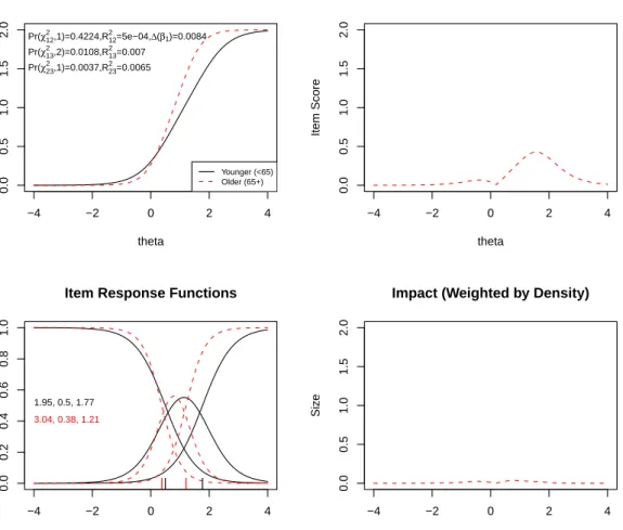
We used the likelihood ratio (LR)χ2_{test (criterion = "Chisqr") as the detection criterion} at the α level of 0.01, and McFadden’s pseudo R2 (default) as the magnitude measure. With a minimum cell count of 5, all items ended up with one or more response categories collapsed. After recoding (done bylordif), four items ended up with four response categories, one item had two categories, and the rest had three. Using these settings, lordif terminated in two iterations flagging five items as displaying age-related DIF – #1 (“I felt fearful”), #9 (“I was anxious if my normal routine was disturbed”), #11 (“I was easily startled”), #18 (“I worried about other people’s reactions to me”), and #24 (“Many situations made me worry”). The standard sum score-based method flagged the same items and one additional item – #7 (“I felt upset”). The plot function in lordif shows (see Figure 1) the theta distributions for the younger and older groups. Older people on average had lower mean scores than their younger counterparts (−0.57 vs. 0.04). Theplot function then displays four diagnostic plots for each of the flagged items (see Figures2–6). The top left plot in Figure2shows item true-score functions based on group-specific item parameter estimates. The slope of the function for the older group was substantially higher than that for the younger group, indicating non-uniform DIF. The LR χ2 test for uniform DIF, comparing Model 1 and Model 2, was

−4 −2 0 2 4 0.0 0.5 1.0 1.5 2.0

Item True Score Functions − Item 1

theta Item Score Younger (<65) Older (65+) Pr(χ12 2 ,1)=0.4224,R₁₂2=5e−04,∆(β1)=0.0084 Pr(χ13 2 ,2)=0.0108,R13 2 =0.007 Pr(χ23 2 ,1)=0.0037,R23 2 =0.0065 −4 −2 0 2 4 0.0 0.5 1.0 1.5 2.0

Difference in Item True Score Functions

theta Item Score −4 −2 0 2 4 0.0 0.2 0.4 0.6 0.8 1.0

Item Response Functions

theta Probability 1.95, 0.5, 1.77 | | 3.04, 0.38, 1.21 | | −4 −2 0 2 4 0.0 0.5 1.0 1.5 2.0

Impact (Weighted by Density)

theta

Siz

e

Figure 2: Graphical display of the item “I felt fearful” which shows non–uniform DIF with respect to age. Note: This item retained three response categories (0, 1, and 2) from the origi-nal five–point rating scale after collapsing the top three response categories due to sparseness. The program by default uses a minimum of five cases per cell (the user can specify a different minimum) in order to retain each response category. The upper–left graph shows the item characteristic curves (ICCs) for the item for older (dashed curve) vs. younger (solid curve). The upper–right graph shows the absolute difference between the ICCs for the two groups, indicating that the difference is mainly at high levels of anxiety (theta). The lower–left graph shows the item response functions for the two groups based on the demographic–specific item parameter estimates (slope and category threshold values by group), which are also printed on the graph. The lower–right graph shows the absolute difference between the ICCs (the upper–right graph) weighted by the score distribution for the focal group, i.e., older individ-uals (dashed curve in Figure 1), indicating minimal impact. See text for more details.

not significant (p = 0.42), whereas the 1-df test for comparing Model 2 and Model 3 was significant (p = 0.0004). It is interesting to note that had the 2-df test (comparing Models 1 and 3) been used as the criterion for flagging, this item would not have been flagged at

−4 −2 0 2 4 0.0 0.5 1.0 1.5 2.0

Item True Score Functions − Item 9

theta Item Score Younger (<65) Older (65+) Pr(χ12 2 ,1)=2e−04,R₁₂2=0.0094,∆(β1)=0.066 Pr(χ13 2 ,2)=0.001,R13 2 =0.0094 Pr(χ23 2 ,1)=0.9692,R23 2 =0 −4 −2 0 2 4 0.0 0.5 1.0 1.5 2.0

Difference in Item True Score Functions

theta Item Score −4 −2 0 2 4 0.0 0.2 0.4 0.6 0.8 1.0

Item Response Functions

theta Probability 1.75, 0.23, 1.1 | | 1.46, −0.31, 1.1 | | −4 −2 0 2 4 0.0 0.5 1.0 1.5 2.0

Impact (Weighted by Density)

theta

Siz

e

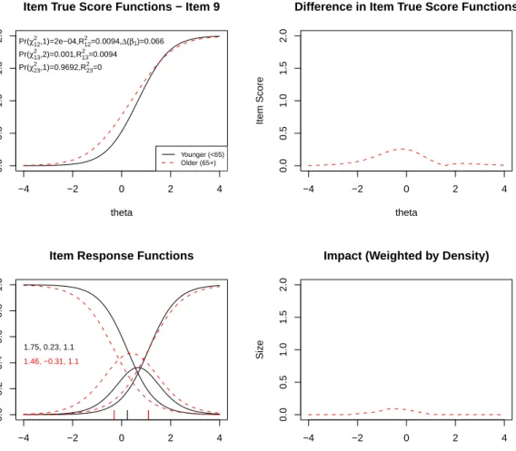
Figure 3: Graphical display of the item “I was anxious if my normal routine was disturbed” which shows uniform DIF with respect to age. Note: See detailed comments accompanying Figure 2. Here the differences between younger and older individuals appear to be at lower anxiety levels.

The bottom left plot in Figure 2 juxtaposes the item response functions for younger and older adults. The non-uniform component of DIF revealed by the LR χ2 _{test can also be} observed in the difference of the slope parameter estimates (3.04 vs. 1.95). Although there was no significant uniform DIF, on close inspection the difference in the second category threshold values (shown as hash marks immediately above the x-axis) for the two groups were noticeable (1.21 vs. 1.77). For polytomous items, a single item-level index of DIF may not provide adequate information concerning which response categories (or score levels) contribute to the DIF effect. The combination of visual and model-based approaches in lordif provide useful diagnostic information at the response category level, which can be systematically investigated under the differential step functioning framework (Penfield 2007; Penfieldet al. 2009).

The top right plot in Figure2presents the expected impact of DIF on scores as the absolute difference between the item true–score functions (Kim et al. 2007). There is a difference in

−4 −2 0 2 4 0.0 0.5 1.0 1.5 2.0

Item True Score Functions − Item 11

theta Item Score Younger (<65) Older (65+) Pr(χ12 2 ,1)=3e−04,R₁₂2=0.0087,∆(β1)=0.0608 Pr(χ13 2 ,2)=0.0016,R13 2 =0.0087 Pr(χ23 2 ,1)=0.9236,R23 2 =0 −4 −2 0 2 4 0.0 0.5 1.0 1.5 2.0

Difference in Item True Score Functions

theta Item Score −4 −2 0 2 4 0.0 0.2 0.4 0.6 0.8 1.0

Item Response Functions

theta Probability 1.3, 0.29, 1.85 | | 1.49, −0.33, 1.23 | | −4 −2 0 2 4 0.0 0.5 1.0 1.5 2.0

Impact (Weighted by Density)

theta

Siz

e

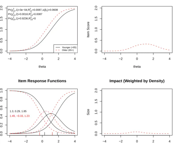
Figure 4: Graphical display of the item “I was easily startled” which shows uniform DIF with respect to age. Note: See detailed comments accompanying Figure2. Here the differ-ences between younger and older individuals are across almost the entire spectrum of anxiety measured by the test.

the item true–score functions peaking at approximately θ = 1.5, but the density–weighted impact (shown in the bottom right plot) is negligible because few subjects have that trait level in this population. When weighted by the focal group trait distribution the expected impact became negligible, which is also apparent in the small McFadden’s pseudoR2measures (printed on the top left plot), i.e., R2₁₃= 0.007 andR2₂₃ = 0.006. Figure 3 displays the plots for item #9 (“I was anxious if my normal routine was disturbed”), which shows statistically significant uniform DIF, P r(χ2₁₂,2) < 0.001. The LR χ2₁₃ was also significant; however, as the LRχ2₂₃was non–significant this result suggests the DIF was primarily uniform. The item response functions suggest that uniform DIF was due to the first category threshold value for the focal group being smaller than that for the reference group (−0.31 vs. +0.23). Figure 4

displays slightly stronger uniform DIF for item #11 (“I was easily startled”). Again, both

χ2₁₂ and χ2₁₃ were significant (p < 0.001) with non–significant χ2₂₃. McFadden’s R2 change for uniform DIF was 0.009, which is considered a negligible effect size (Cohen 1988). The

−4 −2 0 2 4

0.0

1.0

2.0

3.0

Item True Score Functions − Item 18

theta Item Score Younger (<65) Older (65+) Pr(χ12 2 ,1)=0.0027,R₁₂2=0.0048,∆(β1)=0.0238 Pr(χ13 2 ,2)=0.0103,R13 2 =0.0048 Pr(χ23 2 ,1)=0.7036,R23 2 =1e−04 −4 −2 0 2 4 0.0 1.0 2.0 3.0

Difference in Item True Score Functions

theta Item Score −4 −2 0 2 4 0.0 0.2 0.4 0.6 0.8 1.0

Item Response Functions

theta Probability 1.34, −0.41, 0.67, 2.09 | | | 1.39, −0.03, 1.34, 2.88 | | | −4 −2 0 2 4 0.0 1.0 2.0 3.0

Impact (Weighted by Density)

theta

Siz

e

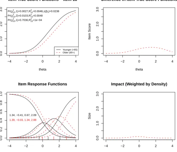
Figure 5: Graphical display of the item “I worried about other people’s reactions to me” which shows uniform DIF with respect to age. Note: See detailed comments accompanying Figure2.

item response functions show that the category threshold parameters for the focal group were uniformly smaller than those for the reference group. Figure 5 displays another item with uniform DIF, item#18 (“I worried about other people’s reactions to me”), but in the opposite direction. The item true–score functions reveal that older people are prone to endorse the item with higher categories compared to younger people with the same overall anxiety level. The item response functions also show that the category threshold parameters for the focal group were uniformly higher than they were for the reference group. Finally, Figure6displays uniform DIF for item#24 (“Many situations made me worry”)–both χ2₁₂ and χ2₁₃ tests were statistically significant (p < 0.001) with a non–significant χ2₂₃. However, the item response functions (and the item parameter estimates) revealed a somewhat different diagnosis–the difference in slope parameters (2.80 vs. 1.88) suggests non–uniform DIF.

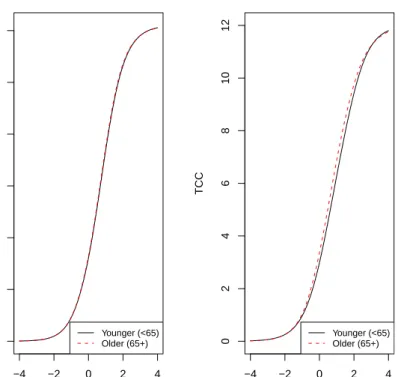
The diagnostic plots for individual DIF items (see Figures2through 6) are followed inlordif by two test–level plots. Figure7shows the impact of all of the DIF items on test characteristic curves (TCCs). The left plot is based on item parameter estimates for all 29 items including the group–specific parameter estimates for the five items identified with DIF. The plot on the

−4 −2 0 2 4

0.0

1.0

2.0

3.0

Item True Score Functions − Item 24

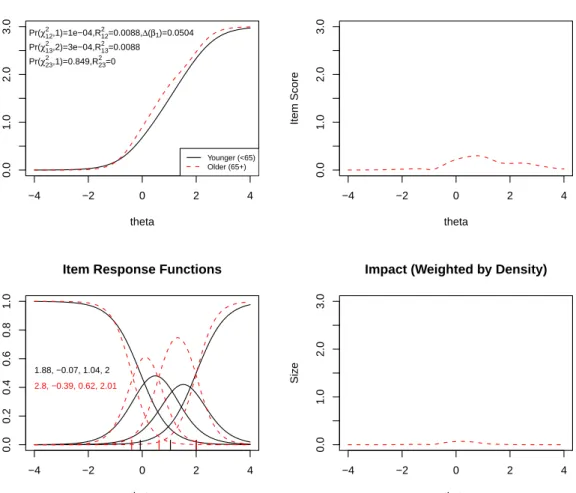
theta Item Score Younger (<65) Older (65+) Pr(χ12 2 ,1)=1e−04,R₁₂2=0.0088,∆(β1)=0.0504 Pr(χ13 2 ,2)=3e−04,R13 2 =0.0088 Pr(χ23 2 ,1)=0.849,R23 2 =0 −4 −2 0 2 4 0.0 1.0 2.0 3.0

Difference in Item True Score Functions

theta Item Score −4 −2 0 2 4 0.0 0.2 0.4 0.6 0.8 1.0

Item Response Functions

theta Probability 1.88, −0.07, 1.04, 2 | | | 2.8, −0.39, 0.62, 2.01 | | | −4 −2 0 2 4 0.0 1.0 2.0 3.0

Impact (Weighted by Density)

theta

Siz

e

Figure 6: Graphical display of the item “Many situations made me worry” displaying uniform DIF with respect to age. Note: See detailed comments accompanying Figure2.

right is based only on the group–specific parameter estimates. Although the impact shown in the plot on the right is very small, the difference in the TCCs implies that older adults would score slightly lower (less anxious) if age group–specific item parameter estimates were used for scoring. When aggregated over all the items in the test (left plot) or over the subset of items found to have DIF (right plot), differences in item characteristic curves (Figure7) may become negligibly small due to canceling of differences in opposite directions, which is what appears to have happened here. However, it is possible for the impact on trait estimates to remain.

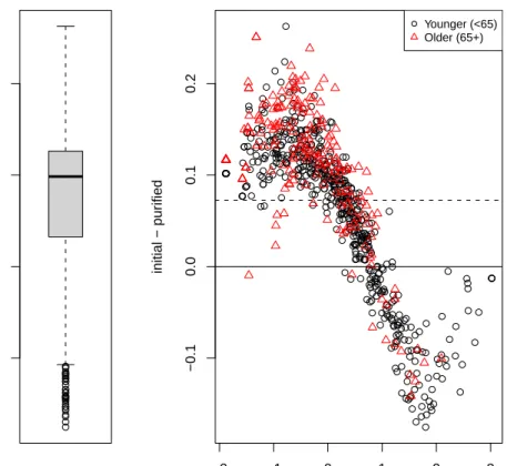
For the impact at the individual score level,lordif compares the initial naive theta estimate and the “purified” theta estimates from the final run accounting for DIF as shown in Figure8. Notice that the item parameter estimates from the final run were equated (using non–DIF items as anchor items) to the initial, single–group calibration and not re–centered to 0.0 (see Step 8), and hence the mean difference (“initial minus purified”) is not necessarily 0.0. This is a modification from the original difwithpar framework (Craneet al. 2006). The Box–and– Whisker plot on the left shows the median difference (over all examinees) is about 0.1 and

−4 −2 0 2 4 0 10 20 30 40 50 60 All Items theta TCC Younger (<65) Older (65+) −4 −2 0 2 4 0 2 4 6 8 10 12 DIF Items theta TCC Younger (<65) Older (65+)

Figure 7: Impact of DIF items on test characteristic curves. Note: These graphs show test characteristic curves (TCCs) for younger and older individuals using demographic–specific item parameter estimates. TCCs show the expected total scores for groups of items at each anxiety level (theta). The graph on the left shows these curves for all of the items (both items with and without DIF), while the graph on the right shows these curves for the subset of these items found to have DIF. These curves suggest that at the overall test level there is minimal difference in the total expected score at any anxiety level for older or younger individuals.

the differences ranged from −0.176 to +0.263 with a mean of 0.073. The scatter plot on the right shows that the final theta estimates had a slightly larger standard deviation (1.122 vs. 1.056). The dotted horizontal reference line is drawn at the mean difference between the initial and purified estimates (i.e., 0.073). With the inclusion of five items with group–specific item parameters, scores at both extremes became slightly more extreme. Accounting for DIF by using group–specific item parameters had negligible effects on individual scores. In the absence of a clinical effect size, we labeled individual changes as “salient” if they exceeded the median standard error (0.198) of the initial score. About 1.96% (15 of 766) of the subjects had salient changes. About 0.52% (4 out of 766) had score changes larger than their initial standard error estimates. Cohen’s effect sizedfor the difference between the two group means (Younger minus Older) was nearly unchanged after identifying and accounting for DIF (from 0.544 to 0.561).

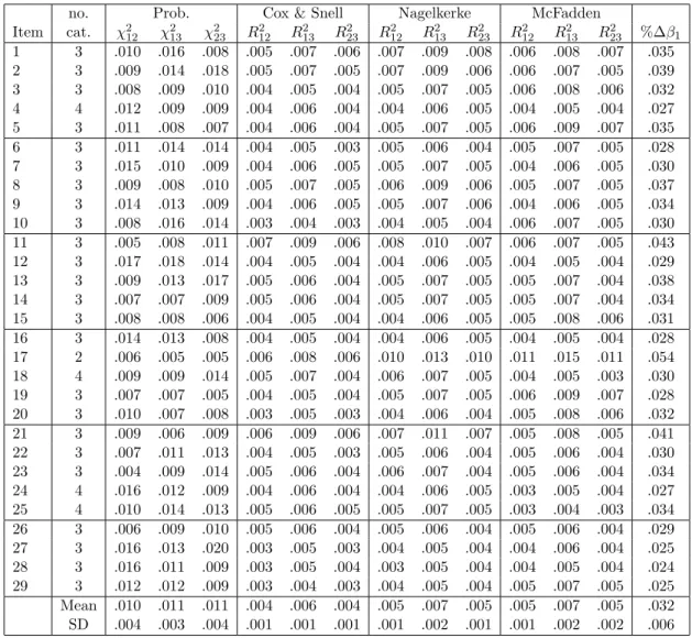
Table1shows the Monte Carlo threshold values for the statistics and magnitude measures by item, based onnr = 1000andalpha = 0.01. On average, the empirical threshold values for

● ● ● ● ● ● ● ● ● ● ● ● ● ● ● ● ● ● ● ● ● ● ● ● ● ● ● ● ● ● ● ● ● −0.1 0.0 0.1 0.2 −2 −1 0 1 2 3 −0.1 0.0 0.1 0.2 initial theta initial − pur ified ● ● ● ● ● ● ● ● ●● ● ● ● ● ● ● ● ● ● ● ● ● ● ● ● ● ● ● ● ● ● ● ● ● ● ● ● ● ● ● ● ● ● ● ● ● ● ● ● ● ● ● ● ● ● ● ● ● ● ● ● ● ● ● ● ● ● ● ● ● ● ● ● ● ● ● ● ● ● ● ● ● ● ● ● ● ● ● ● ● ● ● ● ● ● ● ● ● ● ● ● ● ● ● ● ● ● ● ● ● ● ● ● ● ● ● ● ● ● ● ● ● ● ● ●● ● ● ● ● ● ● ● ● ● ● ● ● ● ● ● ● ● ● ● ● ● ● ● ● ● ● ● ● ● ● ● ● ● ● ● ● ● ● ● ● ● ● ● ● ● ● ● ● ● ● ● ● ● ● ● ● ● ● ● ● ● ● ● ● ● ● ● ● ● ● ● ● ● ● ● ● ● ● ● ● ● ● ● ● ● ● ● ● ● ● ● ● ● ● ● ● ● ● ● ● ● ● ● ● ● ● ● ● ● ● ● ● ● ● ● ● ● ● ● ● ● ● ● ● ● ● ● ● ● ● ● ● ● ● ● ● ● ● ● ● ● ● ● ● ● ● ● ● ● ● ● ● ● ● ● ● ● ● ● ● ● ● ● ● ● ● ● ● ● ● ● ● ● ● ● ● ● ● ● ● ● ● ● ● ● ●● ● ● ● ● ● ● ● ● ● ● ● ● ● ● ● ● ● ● ● ● ● ● ● ● ● ● ● ● ● ● ● ● ● ● ● ● ● ● ● ● ● ● ● ● ● ● ● ● ● ● ● ● ● ● ● ● ● ● ● ● ● ● ● ● ● ● ● ● ● ● ● ● ● ● ● ● ● ● ● ● ● ● ● ● ● ● ● ● ● ●_● ● ● ● ● ● ● ● ● ● ● ● ● ● ● ● ● ● ● ● ●● ● ● ● ● ● ● ● ● ● ● ● ● ● ● ● ● ● ● ● ● ● ● ● ● ● ● ● ● ● ● ● ● ● ● ● ● ● ● ● ● ● ● ● ● ● ● ● ● ● ● ● ● ● ● ● ● ● ● ● ● ● ● ● ● ● ● ● ● ● ● ● ● ● ● ● ● ●● ● ● ● ● ● ● ● ● ● ● ● ● ● ● ● ● ● ● ● ● ● ● ● ● ● ● ● ● ● ● ● ● ● ● ● ● ● ● ● ● ● ● ● ● ● ● ● ● ● ● ● ● ● _{Younger (<65)} Older (65+)

Figure 8: Individual–level DIF impact. Note: These graphs show the difference in score between using scores that ignore DIF and those that account for DIF. The graph on the left shows a box plot of these differences. The interquartile range, representing the middle 50% of the differences (bound between the bottom and top of the shaded box), range roughly from +0.03 to +0.12 with a median of approximately +0.10. In the graph on the right the same difference scores are plotted against the initial scores ignoring DIF (“initial theta”), separately for younger and older individuals. Guidelines are placed at 0.0 (solid line), i.e., no difference, and the mean of the differences (dotted line). The positive values to the left of this graph indicate that in almost all cases, accounting for DIF led to slightly lower scores (i.e., naive score ignoring DIF minus score accounting for DIF > 0, so accounting for DIF score is less than the naive score) for those with lower levels of anxiety, but this appears to be consistent across older and younger individuals. The negative values to the right of this graph indicate that for those with higher levels of anxiety, accounting for DIF led to slightly higher scores, but this again was consistent across older and younger individuals.

the probability associated with the χ2 statistic were close to the nominal α level–the mean probability threshold values across items were 0.010, 0.011, and 0.011 for χ₁₂2 ,χ2₁₃, and χ2₂₃, respectively. Figure 9displays the probability thresholds for the three χ2 statistics by item. The horizontal reference line is drawn at the nominalαlevel (i.e., 0.01). There is no indication

no. Prob. Cox & Snell Nagelkerke McFadden Item cat. χ2₁₂ χ2₁₃ χ₂₃2 R2₁₂ R2₁₃ R2₂₃ R2₁₂ R2₁₃ R2₂₃ R₁₂2 R2₁₃ R2₂₃ %∆β1 1 3 .010 .016 .008 .005 .007 .006 .007 .009 .008 .006 .008 .007 .035 2 3 .009 .014 .018 .005 .007 .005 .007 .009 .006 .006 .007 .005 .039 3 3 .008 .009 .010 .004 .005 .004 .005 .007 .005 .006 .008 .006 .032 4 4 .012 .009 .009 .004 .006 .004 .004 .006 .005 .004 .005 .004 .027 5 3 .011 .008 .007 .004 .006 .004 .005 .007 .005 .006 .009 .007 .035 6 3 .011 .014 .014 .004 .005 .003 .005 .006 .004 .005 .007 .005 .028 7 3 .015 .010 .009 .004 .006 .005 .005 .007 .005 .004 .006 .005 .030 8 3 .009 .008 .010 .005 .007 .005 .006 .009 .006 .005 .007 .005 .037 9 3 .014 .013 .009 .004 .006 .005 .005 .007 .006 .004 .006 .005 .034 10 3 .008 .016 .014 .003 .004 .003 .004 .005 .004 .006 .007 .005 .030 11 3 .005 .008 .011 .007 .009 .006 .008 .010 .007 .006 .007 .005 .043 12 3 .017 .018 .014 .004 .005 .004 .004 .006 .005 .004 .005 .004 .029 13 3 .009 .013 .017 .005 .006 .004 .005 .007 .005 .005 .007 .004 .038 14 3 .007 .007 .009 .005 .006 .004 .005 .007 .005 .005 .007 .004 .034 15 3 .008 .008 .006 .004 .005 .004 .004 .006 .005 .005 .008 .006 .031 16 3 .014 .013 .008 .004 .005 .004 .004 .006 .005 .004 .005 .004 .028 17 2 .006 .005 .005 .006 .008 .006 .010 .013 .010 .011 .015 .011 .054 18 4 .009 .009 .014 .005 .007 .004 .006 .007 .005 .004 .005 .003 .030 19 3 .007 .007 .005 .004 .005 .004 .005 .007 .005 .006 .009 .007 .028 20 3 .010 .007 .008 .003 .005 .003 .004 .006 .004 .005 .008 .006 .032 21 3 .009 .006 .009 .006 .009 .006 .007 .011 .007 .005 .008 .005 .041 22 3 .007 .011 .013 .004 .005 .003 .005 .006 .004 .005 .006 .004 .030 23 3 .004 .009 .014 .005 .006 .004 .006 .007 .004 .005 .006 .004 .034 24 4 .016 .012 .009 .004 .006 .004 .004 .006 .005 .003 .005 .004 .027 25 4 .010 .014 .013 .005 .006 .005 .005 .007 .005 .003 .004 .003 .034 26 3 .006 .009 .010 .005 .006 .004 .005 .006 .004 .005 .006 .004 .029 27 3 .016 .013 .020 .003 .005 .003 .004 .005 .004 .004 .006 .004 .025 28 3 .016 .011 .009 .003 .005 .004 .003 .005 .004 .004 .005 .004 .024 29 3 .012 .012 .009 .003 .004 .003 .004 .005 .004 .005 .007 .005 .025 Mean .010 .011 .011 .004 .006 .004 .005 .007 .005 .005 .007 .005 .032 SD .004 .003 .004 .001 .001 .001 .001 .002 .001 .001 .002 .002 .006

Table 1: Empirical threshold values from Monte Carlo simulations (nr = 1000, alpha =

0.01).

that the empirical threshold values are systematically deviated from the nominal level, which is congruent with previous research showing that the Type I error rate is well controlled under the likelihood ratio test (Kim and Cohen 1998).

Figure10presents the threshold values on pseudoR2 measures. As expected, data generated under no DIF conditions produced negligibly small pseudo R2 measures, i.e., considerably smaller than Cohen’s guideline for a small effect size (0.02). Although some fluctuations are visible across items, the pseudoR2 thresholds were unmistakably smaller than any guidelines for non–trivial effects. Unlike the ordinary least squaresR2, pseudo R2 measures may lack a reasonable interpretation. For instance, the Cox & Snell (Cox and Snell 1989) pseudoR2

measure cannot attain the value of 1 even if the model fits perfectly and residuals are zero (Mittlb¨ock and Schemper 1996). Although the Nagelkerke formula for pseudoR2 corrects the scale issue, it may still lack an immediate interpretation (Mittlb¨ock and Schemper 1999). Mc-Fadden’s pseudoR2 measure, on the other hand, offers intuitively meaningful interpretations,

● ● ● ● _{● ●} ● ● ● ● ● ● ● ● ● ● ● ● ● ● ● ● ● ● ● ● ● ● ● 0 5 10 15 20 25 30 0.000 0.005 0.010 0.015 0.020 Item Pr( χ12 2 ) ● ● ● ● ● ● ● ● ● ● ● ● ● ● ● ● ● ● ● ● ● ● ● ● ● ● ● ● ● 0 5 10 15 20 25 30 0.000 0.005 0.010 0.015 0.020 Item Pr( χ13 2 ) ● ● ● ● ● ● ● ● ● ● ● ● ● ● ● ● ● ● ● ● ● ● ● ● ● ● ● ● ● 0 5 10 15 20 25 30 0.000 0.005 0.010 0.015 0.020 Pr( χ23 2 )

Figure 9: Monte Carlo thresholds forχ2 probabilities (1,000 replications). Note: The graphs show the probability values for each of the items (shown along the x–axis) associated with the 99th quantile (cutting the largest 1% over 1,000 iterations) of theχ2 statistics generated from Monte Carlo simulations under the no DIF condition (data shown in Table1). The lines connecting the data points are placed to show the fluctuation across items and not to imply a series. The horizontal reference line is placed at the nominal alpha level (0.01).

e.g., proportional reduction in the −2 log–likelihood statistic. However, since the primary interest in the current context is the change in the pseudo R2 measures between two nested models, the scale issue may not be a serious concern. Although further study is needed, it is interesting to note that the empirical thresholds based on Cox & Snell displayed the least amount of variation across items (see Figure 10 and standard deviations at the bottom of Table1).

● ● ● ● ● ● ● ● ● ● ● ● ● _● ● ● ● ● ● ● ● ● ● ● ● ● ● ● ● 0 5 10 15 20 25 30 0.000 0.005 0.010 0.015 Item R2 2 − R1 2 ● _McFadden Nagelkerke Cox & Snell

● _● ● ● ● ● ● ● ● ● ● ● ● ● ● ● ● ● ● ● ● ● ● ● ● ● ● _● ● 0 5 10 15 20 25 30 0.000 0.005 0.010 0.015 Item R3 2 − R1 2 ● ● ● ● ● ● ● ● ● ● ● ● ● ● ● ● ● ● ● ● ● ● ● ● ● ● ● ● ● 0 5 10 15 20 25 30 0.000 0.005 0.010 0.015 R3 2 − R2 2

Figure 10: Monte Carlo thresholds for pseudo R2 (1,000 replications). Note: The graphs show the pseudoR2measures for each of the items (shown along the x–axis) corresponding to the 99th quantile (cutting the largest 1% over 1,000 iterations) generated from Monte Carlo simulations under the no DIF condition. The lines connecting the data points are placed to show the fluctuation across items and not to imply a series.

SD= 0.0063). The maximum change across items was 0.0538 (i.e., about 5% change) and was from item #17, which was also the item with the largest pseudoR2 measures (see Figure11). A 10% change inβ1(i.e., 0.1) has been used previously as the criterion for the presence of uni-form DIF (Craneet al.2004). The proportionateβ1 change effect size is closely related to the pseudoR2₁₂ measures (comparing Model 1 vs. Model 2). The correlation coefficients between the threeR2₁₂ measures and the proportionate β1 change thresholds across items were 0.855, 0.928, and 0.784 for Cox & Snell, Nagelkerke, and McFadden, respectively. The correlation between Nagelkerke’sR2₁₂ and the proportionateβ1 change effect size was especially high. It

Figure 11: Monte Carlo thresholds for proportional beta change (1,000 replications). Note: The graphs show the proportionate β1 change measures for each of the items (shown along the x–axis) corresponding to the 99th quantile (cutting the largest 1% over 1,000 iterations) generated from Monte Carlo simulations under the no DIF condition. The lines connecting the data points are placed to show the fluctuation across items and not to imply a series.

is interesting to note that when the proportionate β1 change thresholds were linearly inter-polated (based on the threshold values in Table1), a 10% change inβ1 is roughly equivalent to 0.02 in Nagelkerke’s R2₁₂. Although the two effect size measures and associated flagging criteria originated in different disciplines, they appear to be consistent in this context.

5. Conclusion

The lordif package is a powerful and flexible freeware platform for DIF detection. Ordinal logistic regression (OLR) provides a flexible and robust framework for DIF detection, espe-cially in conjunction with trait level scores from IRT as the matching criterion (Craneet al. 2006). This OLR/IRT hybrid approach implemented inlordifprovides statistical criteria and various magnitude measures for detecting and measuring uniform and non–uniform DIF. Fur-thermore, the use of an IRT trait score in lieu of the traditional sum score makes this approach more robust and applicable even when responses are missing by design, e.g., block–testing, because unlike raw scores comparable IRT trait scores can be estimated based on different sets of items. The lordif package also introduces Monte Carlo procedures to facilitate the identification of reasonable detection thresholds to determine whether items have DIF based on Type I error rates empirically found in the simulated data. This functionality was not available indifwithpar (Craneet al. 2006).

A multitude of DIF detection techniques have been developed. However, very few are avail-able as an integrated, non–proprietary application, and none offers the range of features of lordif. Of the non–proprietary programs, DIFAS (Penfield 2005) and EZDIF (Waller 1998) are based on the sum score. DIFASimplements a variety of DIF detection techniques based on raw scores for both dichotomous and polytomous items. EZDIF only allows dichotomous items, although it employs a two–stage purification process of the trait estimate. IRTLRDIF (Thissen 2001) uses the IRT parameter invariance framework and directly tests the equality of item parameters, but does not allow for empirical determination of DIF detection criteria.

It should be noted that it is on the basis of its features that we recommendedlordif; we have not conducted any simulations to compare its findings with these programs.

In our illustration, five of 29 items were found to have modest levels of DIF related to age. Findings were very similar between the standard sum score–based method and the iterative hybrid OLR/IRT algorithm. The IRT model–based OLR approach provides a mechanism to diagnose DIF in terms of the impact on IRT parameters. The impact of DIF on the TCC was minimal, though some item characteristic curves (ICCs) clearly demonstrated differences. When accounting for DIF, a very small percentage of the subjects had “salient” score changes. This definition of salience is based on the median standard error of measurement (SEM) for the scale. In this instance, the “scale” is an entire item bank with a relatively small median SEM. When a minimal clinically important difference (MCID) is available for a scale, Crane and colleagues recommend a similar approach, but use the MCID and refer to differences beyond the MCID as “relevant” DIF impact (Crane et al. 2007b). While the MCID for the PROMIS anxiety scale has yet to be determined, it will likely be larger than the value used to indicate salience here (0.198). In that case, the proportion of subjects who will haverelevant

DIF will be even smaller than that found to havesalient DIF, further buttressing our view that DIF related to age is negligible in this dataset.

The Monte Carlo simulation results confirmed that the likelihood ratioχ2 test maintains the Type I error adequately in this dataset. Some pseudoR2values varied across items, but overall they were very small under simulations that assume no DIF. Some pseudoR2values may vary from item to item depending on the number of response categories and the distribution within each response category (Menard 2000), so using a single pseudo R2 _{threshold may result in} varying power across items to detect DIF (Craneet al. 2007b). Monte Carlo simulations can help inform the choice of reasonable thresholds. If a single threshold is to be used across all items, it should be set above the highest value identified in Monte Carlo simulations. For instance, the maximum pseudoR2 in Table 1was 0.015, and thus a reasonable lower bound that would avoid Type I errors might be 0.02, which interestingly corresponds to a small, non–negligible effect size (Cohen 1988).

Subsequent development will be facilitated by the algorithm’s ability to account for DIF using group specific item parameters. Future studies may focus on examining the potential greater impact of DIF in a computer adaptive testing (CAT) framework, and developing a CAT platform that can account for DIF in real time. It will also be interesting to compare the OLR/IRT framework implemented in lordif to other DIF detection techniques based on the IRT parameter invariance assumption, such as IRTLRDIF (Thissen 2001) and DFIT (Raju et al. 2009). For instance, it will be interesting to see how those procedures would diagnose item #24 (see Figure6). As noted previously, this item displayed no non–uniform DIF (p = 0.85); however, the slope parameter estimates appeared quite different (1.88 vs. 2.80).

In conclusion, in this paper we introducelordif, a new freeware package for DIF detection that combines IRT and ordinal logistic regression. The Monte Carlo simulation feature facilitates empirical identification of detection thresholds, which may be helpful in a variety of settings. Standard output graphical displays facilitate sophisticated understanding of the nature of and impact of DIF. We demonstrated the use of the package on a real dataset, and found several anxiety items to have DIF related to age, though they were associated with minimal DIF impact.

Acknowledgments

This study was supported in part by the Patient-Reported Outcomes Measurement Informa-tion System (PROMIS). PROMIS is an NIH Roadmap initiative to develop a computerized system measuring PROs in respondents with a wide range of chronic diseases and demographic characteristics. PROMIS II was funded by cooperative agreements with a Statistical Center (Northwestern University, PI: David F. Cella, PhD, 1U54AR057951), a Technology Center (Northwestern University, PI: Richard C. Gershon, PhD, 1U54AR057943), a Network Cen-ter (American Institutes for Research, PI: Susan (San) D. Keller, PhD, 1U54AR057926) and thirteen Primary Research Sites (State University of New York, Stony Brook, PIs: Joan E. Broderick, PhD and Arthur A. Stone, PhD, 1U01AR057948; University of Washington, Seat-tle, PIs: Heidi M. Crane, MD, MPH, Paul K. Crane, MD, MPH, and Donald L. Patrick, PhD, 1U01AR057954; University of Washington, Seattle, PIs: Dagmar Amtmann, PhD and Karon Cook, PhD1U01AR052171; University of North Carolina, Chapel Hill, PI: Darren A. DeWalt, MD, MPH, 2U01AR052181; Children’s Hospital of Philadelphia, PI: Christopher B. Forrest, MD, PhD, 1U01AR057956; Stanford University, PI: James F. Fries, MD, 2U01AR052158; Boston University, PIs: Stephen M. Haley, PhD and David Scott Tulsky, PhD1U01AR057929; University of California, Los Angeles, PIs: Dinesh Khanna, MD and Brennan Spiegel, MD, MSHS, 1U01AR057936; University of Pittsburgh, PI: Paul A. Pilkonis, PhD, 2U01AR052155; Georgetown University, Washington DC, PIs: Carol. M. Moinpour, PhD and Arnold L. Poto-sky, PhD, U01AR057971; Children’s Hospital Medical Center, Cincinnati, PI: Esi M. Morgan Dewitt, MD, 1U01AR057940; University of Maryland, Baltimore, PI: Lisa M. Shulman, MD, 1U01AR057967; and Duke University, PI: Kevin P. Weinfurt, PhD, 2U01AR052186). NIH Science Officers on this project have included Deborah Ader, PhD, Vanessa Ameen, MD, Susan Czajkowski, PhD, Basil Eldadah, MD, PhD, Lawrence Fine, MD, DrPH, Lawrence Fox, MD, PhD, Lynne Haverkos, MD, MPH, Thomas Hilton, PhD, Laura Lee Johnson, PhD, Michael Kozak, PhD, Peter Lyster, PhD, Donald Mattison, MD, Claudia Moy, PhD, Louis Quatrano, PhD, Bryce Reeve, PhD, William Riley, PhD, Ashley Wilder Smith, PhD, MPH, Susana Serrate-Sztein,MD, Ellen Werner, PhD and James Witter, MD, PhD. This manuscript was reviewed by PROMIS reviewers before submission for external peer review. See the Web site athttp://www.nihpromis.org/for additional information on the PROMIS initiative. Additional support for the second and third authors were provided by P50 AG05136 (Raskind) and R01 AG 029672 (Crane). The authors appreciate the careful efforts of Shubhabrata Mukherjee, PhD, to format the manuscript in LA_TEX.

References

Agresti A (1990). Categorical Data Analysis. John Wiley & Sons, New York.

Andersen RB (1967). “On the Comparability of Meaningful Stimuli in Cross-Cultural Re-search.”Sociometry,30, 124–136.

Bjorner JB, Smith KJ, Orlando M, Stone C, Thissen D, Sun X (2006). IRTFIT: A Macro for Item Fit and Local Dependence Tests under IRT Models. Quality Metric Inc, Lincoln, RI.

Camilli G, Shepard LA (1994). Methods for Identifying Biased Test Items. Sage, Thousand Oaks.

Cohen J (1988). Statistical Power Analysis for the Behavioral Sciences. 2nd edition. Lawrence Earlbaum Associates, Hillsdale, NJ.

Cook K (1999). “A Comparison of Three Polytomous Item Response Theory Models in the Context of Testlet Scoring.”Journal of Outcome Measurement,3, 1–20.

Cox DR, Snell EJ (1989). The Analysis of Binary Data. 2nd edition. Chapman and Hall, London.

Crane PK, Cetin K, Cook K, Johnson K, Deyo R, Amtmann D (2007a). “Differential Item Functioning Impact in a Modified Version of the Roland-Morris Disability Questionnaire.”

Quality of Life Research,16(6), 981–990.

Crane PK, Gibbons LE, Jolley L, van Belle G (2006). “Differential Item Functioning Analysis with Ordinal Logistic Regression Techniques: DIF Detect and difwithpar.” Medical Care, 44(11 Supp 3), S115–S123.

Crane PK, Gibbons LE, Narasimhalu K, Lai JS, Cella D (2007b). “Rapid Detection of Differ-ential Item Functioning in Assessments of Health-Related Quality of Life: The Functional Assessment of Cancer Therapy.”Quality of Life Research,16(1), 101–114.

Crane PK, Gibbons LE, Ocepek-Welikson K, Cook K, Cella D (2007c). “A Comparison of Three Sets of Criteria for Determining the Presence of Differential Item Functioning Using Ordinal Logistic Regression.”Quality of Life Research,16(Supp 1), 69–84.

Crane PK, Gibbons LE, Willig JH, Mugavero MJ, Lawrence ST, Schumacher JE, Saag MS, Kitahata MM, Crane HM (2010). “Measuring Depression and Depressive Symptoms in HIV-Infected Patients as Part of Routine Clinical Care Using the 9-Item Patient Health Questionnaire (PHQ-9).”AIDS Care,22(7), 874–885.

Crane PK, Narasimhalu K, Gibbons LE, Mungas DM, Haneuse S, Larson EB, Kuller L, Hall K, van Belle G (2008a). “Item Response Theory Facilitated Cocalibrating Cognitive Tests and Reduced Bias in Estimated Rates of Decline.”Journal of Clinical Epidemiology,61(10), 1018–1027.

Crane PK, Narasimhalu K, Gibbons LE, Pedraza O, Mehta KM, Tang Y, Manly JJ, Reed BR, Mungas DM (2008b). “Composite Scores for Executive Function Items: Demographic Heterogeneity and Relationships with Quantitative Magnetic Resonance Imaging.”Journal of International Neuropsycholigal Society,14(5), 746–759.

Crane PK, van Belle G, Larson EB (2004). “Test Bias in a Cognitive Test: Differential Item Functioning in the CASI.”Statistics in Medicine,23, 241–256.

De Boeck P, Wilson M (2004). Explanatory Item Response Models: A Generalized Linear and Nonlinear Approach. Springer-Verlag, New York.

Donoghue JR, Holland PW, Thayer DT (1993). “A Monte Carlo Study of Factors That Affect the Mantel-Haenszel and Standardization Measures of Differential Item Functioning.” In

P Holland, H Wainer (eds.),Differential Item Functioning, pp. 137–166. Erlbaum, Hillsdale, NJ.

Dorans NJ, Holland PW (1993). “DIF Detection and Description: Mantel-Haenszel and Standardization.” In P Holland, H Wainer (eds.),Differential Item Functioning, pp. 35–66. Erlbaum, Hillsdale, NJ.

French AW, Miller TR (1996). “Logistic Regression and Its Use in Detecting Differential Item Functioning in Polytomous Items.”Journal of Educational Measurement,33, 315–332. French BF, Maller SJ (2007). “Iterative Purification and Effect Size Use with Logistic

Re-gression for Differential Item Functioning Detection.”Educational and Psychological Mea-surement,67(3), 373–393.

Gibbons LE, McCurry S, Rhoads K, Masaki K, White L, Borenstein AR, Larson EB, Crane PK (2009). “Japanese-English Language Equivalence of the Cognitive Abilities Screening Instrument among Japanese-Americans.” International Psychogeriatrics,21(1), 129–137. Gregorich SE (2006). “Do Self-Report Instruments Allow Meaningful Comparisons across

Di-verse Population Groups? Testing Measurement Invariance Using the Confirmatory Factor Analysis Framework.”Medical Care,44(11 Supp 3), S78–S94.

Harrell Jr FE (2009).Design: Design Package.Rpackage version 2.3-0, URLhttp://CRAN. R-project.org/package=Design.

Holland PW, Thayer DT (1988). “Differential Item Prformance and the Mantel-Haenszel Procedure.” In H Wainer, HI Braun (eds.),Test Validity, pp. 129–145. Erlbaum, Hillsdale, NJ.

Jodoin MG, Gierl MJ (2001). “Evaluating Type I Error and Power Rates Using an Effect Size Measure with the Logistic Regression Procedure for DIF Detection.”Applied Measurement in Education,14, 329–349.

Jones R (2006). “Identification of Measurement Differences between English and Spanish Lan-guage Versions of the Mini-Mental State Examination: Detecting Differential Item Func-tioning Using MIMIC Modeling.”Medical Care,44, S124–S133.

Kang T, Chen T (2008). “Performance of the GeneralizedS−X2 Item Fit Index for Polyto-mous IRT Models.”Journal of Educational Measurement,45(4), 391–406.

Kim SH, Cohen AS (1998). “Detection of Differential Item Functioning under the Graded Response Model with the Likelihood Ratio Test.”Applied Psychological Measurement,22, 345–355.

Kim SH, Cohen AS, Alagoz C, Kim S (2007). “DIF Detection Effect Size Measures for Polytomously Scored Items.”Journal of Educational Measurement,44(2), 93–116.

Li H, Stout W (1996). “A New Procedure for Detection of Crossing DIF.” Psychometrika, 61, 647–677.

Lord FM (1980). Applications of Item Response Theory to Practical Testing Problems. Lawrence Erlbaum Associates, Hillsdale, NJ.