The application of visual saliency models in objective image quality assessment: a statistical evaluation

Wei Zhang, Student Member, IEEE, Ali Borji, Member, IEEE, Zhou Wang, Fellow, IEEE,

Patrick Le Callet, Senior Member, IEEE, and Hantao Liu, Member, IEEE

Abstract— Advances in image quality assessment have shown

the potential added value of including visual attention aspects in its objective assessment. Numerous models of visual saliency are implemented and integrated in different image quality metrics (IQMs), but the gain in reliability of the resulting IQMs varies to a large extent. The causes and the trends of this variation would be highly beneficial for further improvement of IQMs, but are not fully understood. In this paper, an exhaustive statistical evaluation is conducted to justify the added value of computational saliency in objective image quality assessment, using 20 state-of-the-art saliency models and 12 best-known IQMs. Quantitative results show that the difference in predicting human fixations between saliency models is sufficient to yield a significant difference in performance gain when adding these saliency models to IQMs. However, surprisingly, the extent to which an IQM can profit from adding a saliency model does not appear to have direct relevance to how well this saliency model can predict human fixations. Our statistical analysis provides useful guidance for applying saliency models in IQMs, in terms of the effect of saliency model dependence, IQM dependence, and image distortion dependence. The testbed and software are made publicly available to the research community.

Index Terms— Image quality assessment, quality metric,

saliency model, statistical analysis, visual attention.

I. INTRODUCTION

O

VER the past decades, we have witnessed tremendous progress in the development of image quality met-rics (IQMs), which can automatically predict perceived image quality aspects. A variety of IQMs have proven successful in terms of being able to serve as a practical alternative for expensive and time-consuming quality evaluation by human observers. These IQMs are now taking an increasingly Manuscript received September 30, 2014; revised June 27, 2015; accepted July 18, 2015.

W. Zhang and H. Liu are with the School of Computer Sci-ence and Informatics, Cardiff University, CF24 3AA, U.K. (e-mail: [email protected]; [email protected]).

A. Borji is with the Department of Computer Science, University of Central Florida, Orlando, FL 32816 USA (e-mail: [email protected]).

Z. Wang is with the Department of Electrical and Computer Engineering, University of Waterloo, Waterloo, ON N2L3G1, Canada (e-mail: [email protected]).

P. Le Callet is with the IRCCyN Laboratory, University of Nantes, Nantes 44300, France (e-mail: [email protected]).

Color versions of one or more of the figures in this paper are available online at http://ieeexplore.ieee.org.

Digital Object Identifier 10.1109/TNNLS.2015.2461603

important role in digital imaging systems for a broad range of applications, e.g., for the optimization of video chains, the benchmarking and standardization of image and video processing algorithms, and the quality monitoring and control in displays [2]. They range from dedicated IQMs that assess a specific type of image distortion to general IQMs that measure the overall perceived quality. Both the dedicated and the general IQMs can be classified into full-reference (FR), reduced reference (RR), and no-reference (NR) metrics, depending on to what extent they use the original, distortion-free image material as [2]. FR metrics assume the reference is fully accessible, and they are based on measuring the similarity or fidelity between the distorted image and its original. RR metrics are mainly used in scenarios where the reference is partially available, e.g., in complex communication networks. They make use of certain features extracted from the reference, which are then employed as side information to evaluate the quality of the distorted image. In many real-world applications, however, there is no access to the reference at all. Hence, it is desirable to have NR metrics that can assess the overall quality or some aspects of it based on the distorted image only.

Since the human visual system (HVS) is the ultimate assessor of image quality, the effectiveness of an IQM is generally quantified by to what extent its quality prediction is in agreement with human judgements [2]. In this respect, researchers have taken different approaches to predict the perceived image quality mainly by including the functional aspects of the HVS. Advances in human vision research have increased our understanding of the mechanisms of the HVS, and allowed expressing these psychophysical findings into mathematical models [3]–[5]. Some well-established models that address the lower level aspects of early vision, such as contrast sensitivity, luminance masking, and texture masking, are integrated in the design of various IQMs [6]–[10]. These so-called HVS-based IQMs are claimed to be much more reliable than the purely pixel-based IQMs, such as peak signal-to-noise ratio (PSNR). This approach, however, remains limited in its sophistication, and thus also in its reliability, mainly due to our limited knowledge of the HVS, which makes it nearly impossible to precisely simulate all image quality perception-related components. Instead of imitating the func-tional operations of the HVS, alternative approaches are based 2162-237X © 2016 IEEE. Personal use is permitted, but republication/redistribution requires IEEE permission.

on modeling the overall functionality of the HVS [11]–[18], e.g., by utilizing the observation that the HVS is highly adapted to extract the structural information from visual scenes [11]. It has been demonstrated that these IQMs are rather effective in predicting perceived image quality.

To further improve the reliability of IQMs, a signifi-cant current research trend is to investigate the impact of visual attention, which refers to a process that enables the HVS to select the most relevant information from a visual scene [19]–[27]. Compared with what is known about many other aspects of the HVS in IQMs, our knowledge on modeling visual attention in the IQM design is, however, very limited. This is primarily due to the fact that how human attention affects the perception of image quality is unknown, and also due to the difficulties of precisely simulating visual attention. Researchers now attempt to simplify this problem by incorpo-rating visual attention aspects into IQMs in an ad hoc way, based on optimizing the performance increase in predicting perceived quality [23]–[27]. The approaches taken in the literature, which may be implemented in slightly different ways, are generally based on the assumption that distortion occurring in an area that attracts the viewer’s attention is more annoying than in any other area. They weight local distortions with local saliency, resulting in a more sophisticated means of image quality prediction. It should, however, be noted that this concept strongly relies on the simplification of the HVS that the natural scene saliency (i.e., saliency driven by the original content of the visual scene, and referred to as SS) and the image distortions (i.e., the unnatural artifacts superimposed to the original visual scene) are treated separately and the results are then combined artificially to determine the overall quality. The actual interactions between SS and distortions may be more complex; modeling these interactions is so far limited by our lack of knowledge of the HVS. In addition, to maintain a low computational complexity of an IQM at sufficiently high prediction accuracy, the potential performance increase should be balanced against the additional costs needed for modeling visual attention, including its interactions with distortions. As such, this simplified approach appears to be a viable and, probably so far the most acceptable way of including visual attention aspects in IQMs [23]–[27]. Based on this approach, some researchers resort to eye-tracking data in an attempt to find out the intrinsic added value of visual attention to the reliability of IQMs [19]–[22]. By integrating the measured ground-truth SS into the state-of-the-art IQMs, one could identify whether and to what extent the addition of saliency is beneficial to objective image quality prediction in a genuine manner. A dedicated study in [19] also demonstrates that if saliency is added to IQMs, it should be the SS driven by the original scene content rather than the saliency obtained during scoring the quality of the scene being distorted. This finding arises probably due to the saliency (or distraction power) of the distortions present in an image is already sufficiently addressed in an IQM, and should not be duplicated in the measurement of saliency. This evidence supports our earlier statement that SS and distortions need to be approached as separate components. From a practical point of view, e.g., in a real-time imple-mentation of an IQM, the saliency measured offline with eye

tracking needs to be substituted by a computational model of visual saliency. In this respect, in addition to the eye-tracking data-based results reported in [19], it is worth investigating whether a saliency model, at least with the current soundness of visual saliency modeling, is also able to improve the performance of IQMs, and if so, to what extent. Literature on studying the added value of the computational saliency in IQMs is mainly focused on the extension of a specific IQM with a specific saliency model; a map derived from an IQM that represents the spatial distribution of image distortions is weighted with the calculated saliency [23]–[27]. For example, in [23], a saliency model developed in [29] is adopted to improve a particular IQM [11] in assessing the quality induced by packet loss. To enhance the performance of a sharpness metric in [24], a new saliency model is proposed and integrated in this metric. In [25], a dedicated saliency model is invented to refine two IQMs called visual information fidelity (VIF) [12] and MSSIM [30], resulting in a significant gain in their performance. In both [26] and [27], computational saliency is incorporated in the IQM design to increase its correlation with subjective quality judgements. As shown above, employing a specific saliency model to specifically optimize a target IQM is often effective. There are, however, several concerns related to this approach. First, a variety of saliency models are available in the literature, which is summarized in [31]–[34]. They are either specifically designed or chosen for a specific domain, but the general applicability of these models in the context of image quality assessment is so far not completely investigated. A rather random selection of a particular saliency model runs the risk of compromising the possibly optimal performance gain equivalent to that may be obtained by adding eye-tracking data in IQMs. It is, e.g., not known yet whether the gain in performance (if existing) when adding a chosen saliency model is comparable with its corresponding gain when ground-truth saliency is used. Second, questions still arise whether a saliency model successfully embedded in one particular IQM is also able to enhance the performance of other IQMs, and whether a dedicated combination of a saliency model and an IQM that can improve the assessment of one particular type of image distortion would also improve the assessment of other distortion types. If so, it remains questionable whether the gain obtained by adding this preselected saliency model to a specific IQM (or to IQMs to assess a specific distortion) is comparable with the gain that can be obtained with alternative IQMs (or when assessing other distortion types). Finally, it has been taken for granted in the literature that a saliency model that better predicts human fixations is expected to be more advantageous in improving the performance of IQMs. This speculation, however, has not been statistically validated yet. The various concerns discussed above imply that before implementing saliency models in IQMs, it is desirable to have a comprehensive understanding on whether and to what extent the addition of computational saliency can improve IQMs, in the context of the existing saliency models and IQMs available in the literature.

In this paper, we quest the capability and capacity of com-putational saliency in improving IQM’s performance in pre-dicting perceived image quality. Based on [19], [31], and [32],

Fig. 1. Illustration of saliency maps generated by 20 state-of-the-art saliency models for one of the source images in LIVE database [28].

an exhaustive statistical evaluation is conducted by integrating the state-of-the-art saliency models in several IQMs well known in the literature. We investigate whether there is a significant difference in predicting human fixations between saliency models, and whether and to what extent such dif-ference can affect the actual gain in prediction performance that can be obtained by including saliency in IQMs. The statistics also allow us to explore whether or not there is a direct relation between how well a saliency model can predict human fixations and to what extent an IQM can profit from adding this saliency. Furthermore, we explicitly evaluate to what extent the amount of performance gain when adding computational saliency depends on the saliency model, IQM, and type of image distortion. We intend to, based on in-depth statistical analysis, provide recommendations and practical solutions with respect to the application of saliency models in IQMs. We have made the testbed and software publicly available to facilitate future research in saliency-based IQMs.

II. EVALUATIONFRAMEWORK

To evaluate the added value of computational saliency in IQMs, we follow the general framework established in [19]. In this evaluation, the saliency map derived from a saliency model is integrated into an IQM, and the resulting IQM’s performance is compared with the performance of the same IQM without saliency. To ensure a study of sufficient statistical power, our validation is carried out with 20 saliency models, 12 IQMs, and 3 image quality assessment databases, which are all so far widely accepted in the research community.

A. Visual Saliency Models

The 20 state-of-the-art models of visual saliency, namely AIM, AWS, CBS, EDS, FTS, Gazit, GBVS, CA, SR, DVA, ITTI, SDFS, PQFT, salLiu, SDCD, SDSR, STB, SUN, SVO, and Torralba, are implemented. These models are already described in more detail in [31]–[35], and are only briefly summarized here. ITTI [36] is perhaps the first notable work in the field of computational modeling of visual attention, which combines multiscale image features into a single topographical saliency map. STB [29] is meant to improve the output of ITTI for its use in region of interest (ROI) extraction. Based on the principle of maximizing information sampled in a scene, AIM [37] and SUN [38], which are implemented in slightly different ways, compute saliency using Shannon’s self-information measure of visual features. Similarly, DVA [39] measures saliency with an attempt to maximize the entropy of the sampled visual features. GBVS [40] is based on graph

theory and is achieved by concentrating mass on activation maps, which are formed from certain raw features. The salLiu [41] focuses on the salient object detection (SOD) problem for images, using a conditional random field to learn ROI from a set of predefined features. CA [42] employs both local and global clues to separate the salient object from the background. Torralba [43] contains both local features and global scene context. SR [44] and PQFT [45] are simple yet efficient models, which explore the phase spectrum of Fourier transform. FTS [46] aims for the detection of well-defined boundaries of salient objects, which is achieved by retaining more frequency content from the image. EDS [47] relies on multiscale edge detection and produces a sim-ple and nonparametric method for detecting salient regions. Holtzman-Gazit [48] employs a local-regional multilevel approach to detect edges of salient objects. CBS [49] is formalized as an iterative energy minimization framework, which results in a binary segmentation of the salient object. AWS [50] computes saliency by considering the decorrelation and distinctiveness of multiscale low-level features. SDSR [51] measures the likeness of a pixel to its surroundings. SDFS [52] combines global features from frequency domain and local features from spatial domain. SVO [53] improves SOD by fusing generic objectness and saliency. SDCD [35] works in the compressed domain and adopts intensity, color, and texture features for saliency detection.

Fig. 1 shows the saliency maps generated by the models mentioned above for one of the source images in LIVE image quality assessment database [28]. These models cover a wide range of modeling approaches and application environments. In [33] and [34], they may be generally classified into two categories. One category of saliency models focuses on mimicking the behavior and neuronal architecture of the early primate visual system, aiming to predict human fixations as a way to test its accuracy in saliency detection (e.g., ITTI, AIM, and GBVS). The other category is driven by the practical need of object detection for machine vision applications, attempting to identify explicit salient regions/objects (e.g., FTS, CBS, and SVO).

B. Image Quality Metrics

The 12 widely accepted IQMs, namely PSNR, universal quality index (UQI), SSIM, MSSIM, VIF, feature similarity index (FSIM), IWPSNR, IWSSIM, generalized block-edge impairment metric (GBIM), NR blocking artifact mea-sure (NBAM), NR perceptual blur metric (NPBM), and just noticeable blur metric (JNBM), are applied in our evaluation.

These IQMs include eight FR and four NR metrics, and range from the purely pixel-based IQMs without the characteristics of the HVS to IQMs that contain complex HVS modeling. The FR metrics are as follows.

PSNR: The PSNR is based on the mean squared error

between the distorted image and its original on a pixel-by-pixel basis.

UQI: The UQI [54] measures the image quality degradation

as a combination of the loss of pixel correlation, luminance, and contrast.

SSIM: The structural similarity index [11] measures image

quality based on the degradation in the structural information.

MS-SSIM: The multiscale SSIM [30] represents a refined

and flexible version of the single-scale SSIM, incorporating the variations of viewing conditions.

IWPSNR: PSNR is extended with a pooling strategy

(i.e., the information content weighting as described in [55]) of the locally calculated distortions.

IWSSIM: SSIM is extended with a pooling strategy

(i.e., the information content weighting as described in [55]) of the locally calculated distortions.

VIF: The VIF [12] quantifies how much of the information

present in the reference image can be extracted from the distorted image.

FSIM: The FSIM [56] utilizes the phase congruency and

gradient to calculate the local distortions. The NR metrics are as follows.

GBIM: The GBIM [57] measures a blocking artifact as an

interpixel difference across block boundaries, which is scaled with a weighting function of HVS masking.

NPBM: The NPBM [58] is based on extracting sharp edges

in an image, and measuring the width of these edges.

JNBM: The JNBM [59] refines the measurement of the

spread of the edges by integrating the concept of just noticeable blur.

NBAM: The NBAM [60] considers the visibility of a

blocking artifact by computing the local contrast in gradient. The IQMs mentioned above are implemented in the spatial domain. They estimate image quality locally, resulting in a quantitative distortion map (DM) which represents a spatially varying quality degradation profile. It is noted that other well-known IQMs formulated in the transform domain, such as VSNR [61], MAD [62], and NQM [63], are not included in our study. Integrating a saliency map in a rather complex IQM calculated in the frequency domain is not straightforward, and is therefore, outside the scope of this paper.

C. Image Quality Assessment Databases

The evaluation of the performance of an IQM is conducted on the LIVE database [28]. The reliability of the LIVE database is widely recognized in the image quality community. It consists of 779 images distorted with a variety of distortion types, i.e., JPEG compression (i.e., JPEG), JPEG2000 compression (i.e., JP2K), white noise (WN), Gaussian blur (GBLUR), and simulated fast-fading (FF) Rayleigh occurring in (wireless) channels. Per image the database also gives a difference in mean opinion score (DMOS) derived

from an extensive subjective quality assessment study. Indeed, the image quality community is more and more accustomed to the evaluation of IQMs with different databases that are made publicly available. It may, e.g., account for the innate limitations of a typical subjective experiment in terms of the diversity in image content and distortion type, and therefore, provide more implications on the robustness of an IQM. With this in mind, a cross-database evaluation is carried out by repeating our evaluation protocol on other two existing image quality databases, i.e., IVC [64] and MICT [65], which are customarily used in the literature. It should, however, be noted that the meaningfulness of a cross-database validation heavily depends on, e.g., the consistency between different databases. The measured difference in the performance of an IQM can be attributed to the difference between the designs of different subjective experiments.

D. Evaluation Criteria

1) Predictability of Saliency Models: To quantify the

similarity between a ground-truth human saliency map (HSM) (as described in detail in [19]) obtained from eye-tracking and the modeled saliency map (MSM) (as described in detail in [31]) derived from a saliency model, three measures are often used in the literature. These measures are as follows.

CC: Pearson linear correlation coefficient (CC) (see [66], [67]) measures the strength of a linear relationship between two variables, i.e., HSM and MSM in our case. When CC is close to +1/−1 there is almost a perfect linear relationship between the two maps.

NSS: Normalized scanpath saliency (NSS) (see [68], [69])

checks, per fixation point in the HSM, the value at its cor-responding location in the MSM. This value is normalized to have zero mean and unit standard deviation, and then averaged over all fixation points. Thus, when NSS > 1, the MSM exhibits significantly higher average saliency over the fixation locations than the nonfixation locations, whereas NSS < 0 indicates that the probability that an MSM is able to predict human fixations is likely due to chance.

SAUC: AUC refers to the area under the receiver operating

characteristic curve. Shuffled AUC (i.e., SAUC and defined in [31]) is a refined version of the classical AUC for saliency evaluation. In a conventional AUC measurement, the ground-truth human fixations in an image constitute a positive set, whereas a set of negative points is randomly selected. The MSM is then treated as a binary classifier to separate the pos-itives from the negatives. Because of the more or less centered distribution of the human fixations (e.g., human eye tends to look at the central area of an image and/or photographers often place salient objects in the image center [38]) in a typical image database, a saliency model could take advantage of such the so-called center-bias by weighting its saliency map with a central Gaussian blob. This usually yields a dramatic increase in the AUC score. SAUC is proposed to normalize the effect of center-bias and as a consequence, to ensure a fair comparison of saliency models. Instead of selecting negative points randomly, all fixations over other images in the same database are used as the negative set. By doing so,

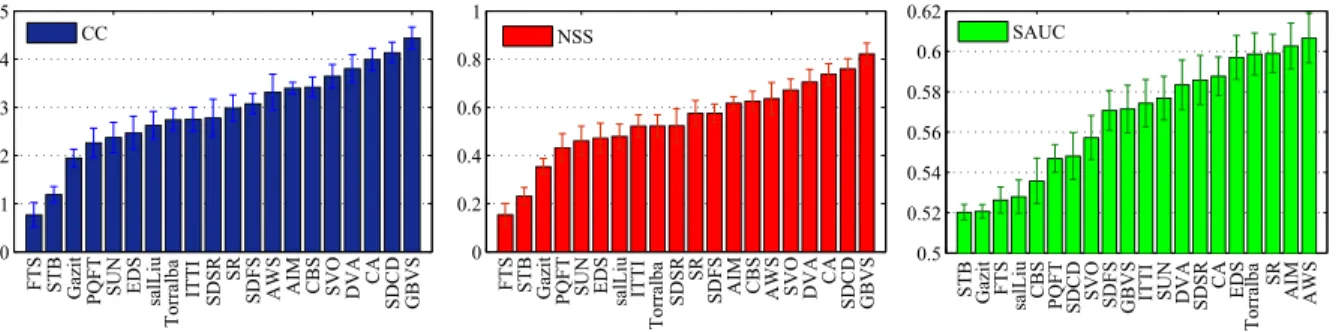
Fig. 2. Illustration of the rankings of visual saliency models (the detail of the models can be found in Section II-A) in terms of CC, NSS, and SAUC, respectively. CC, NSS, and SAUC are calculated based on the eye-tracking database in [19]. Error bars: 95% confidence interval.

SAUC gives more credit to the off center information and favors true positives more. In this regard, SAUC is considered a rigorous measure; the bad performance of a saliency model cannot be masked by simply adding a central Gaussian filter. A perfect prediction of human fixations corresponds to a score of 1, whereas a score of 0.5 indicates a random guess.

2) Performance of IQMs: A saliency model is included in

an IQM to assess the quality of an image of size M × N

pixels via locally weighting (i.e., by multiplying) the DM by the MSM, of which the process can be defined as

WIQ= M x₌1 N y₌1[DM(x,y)×MSM(x,y)] M x=1 N y=1MSM(x,y) (1) where DM is calculated by the IQM, MSM is generated from the original image (note in the case of an NR framework, the MSM is either assumed to be available, which is analogous to RR in practice, or considered to be possibly calculated from the distorted image from separating natural scene and distortion), and WIQ denotes the resulting image quality prediction. It should be noted that the DM and MSM are linearly combined in our evaluation. This combination strategy, as also conventionally used in [19]–[22], is simple and parameter-free, and consequently, fulfills a generic implementation. A more sophisticated combination strategy may further improve IQM’s performance, e.g., in assessing a specific type of distortion. In [70] and [71], by considering the interaction between the scene saliency and the distraction power of the JPEG compression artifacts, a dedicated combination strategy has proven more effective than the linear combination strategy. The increase in such effectiveness is often achieved at the expense of the generality of the combination strategy.

As prescribed by the video quality experts group [72], the performance of an IQM is quantified by the Pearson linear CC and the Spearman rank order CC (SROCC) between the outputs of the IQM and the subjective quality ratings. Seemingly, the image quality community is accustomed to fitting the predictions of an IQM to the subjective scores [72]. A nonlinear mapping may, e.g., account for a possible saturation effect in the quality scores at high quality. It usually yields higher CCs in absolute terms, while generally keeping the relative differences between IQMs [73]. As also explained in [19], without a sophisticated nonlinear fitting, the CCs cannot mask a bad performance of the IQM itself.

To better visualize differences in performance, we avoid any nonlinear fitting and directly calculate correlations between the IQM’s predictions and the DMOS scores.

III. ADDINGCOMPUTATIONALSALIENCY INIQMs: THEOVERALLEFFECT ANDITSSTATISTICAL

MEANINGFULNESS

In this section, we evaluate the overall effect of including computational saliency in IQMs. The evaluation protocol breaks down into three coherent steps. First, we check the difference in predictability between saliency models used. Second, by applying these saliency models to individual IQMs, we validate whether there is a meaningful gain in the performance for the IQMs. Finally, we investigate the relation between two trends being the predictability of saliency models and the profitability of including different saliency models in IQMs.

A. Variation in Predictability Between Saliency Models

The predictability of a saliency model is evaluated using the eye-tracking data in [19], which contains 29 HSMs obtained from 20 human observers looking freely to 29 source images of the LIVE database. Per saliency model, CC, NSS, and SAUC are calculated between the HSM and the MSM, and averaged over the 29 stimuli. Fig. 2 shows the rankings of saliency models in terms of CC, NSS, and SAUC, respectively. It shows that the saliency models vary over a broad range of predictability independent of the measure used. Notwith-standing a slight variation in the ranking order across three measures, there is a strong consistency between different ranking results. Similar trends are reported in [20], in which evidence also indicates that the SAUC accounts for center-bias (as the process explained in Section II-D) and, therefore is considered as a more rigorous measure for validating saliency models [31]. Based on SAUC, hypothesis testing is performed in order to check whether the numerical difference in pre-dictability between saliency models is statistically significant. Before being able to decide on an appropriate statistical test, we evaluate the assumption of normality of the SAUC scores. A simple kurtosis-based criterion (as used in [74]) is used for normality; if the SAUC scores have a kurtosis between 2 and 4, they are assumed to be normally distributed, and the difference between saliency models could be tested with a parametric test,

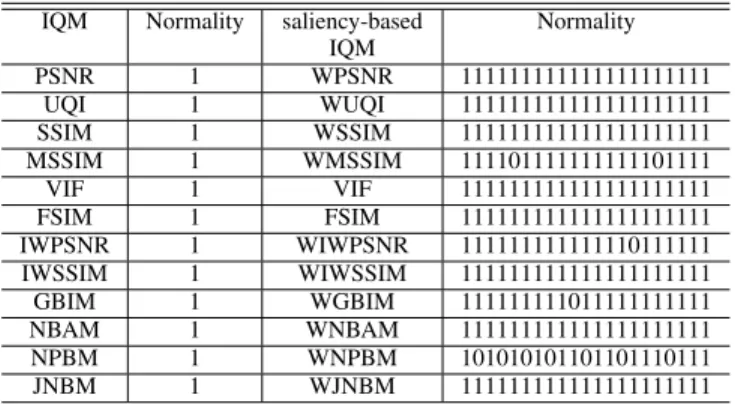
TABLE I

PERFORMANCEGAIN(ASEXPRESSED BY THEINCREASE INCC, i.e.,CC) BETWEEN AMETRIC ANDITSSALIENCY-BASEDVERSION OVERALLDISTORTIONTYPES FOR THEIMAGES OF THELIVE DATABASE. EACHENTRY IN THELASTROWREPRESENTS

THECC AVERAGEDOVERALLSALIENCYMODELSEXCLUDING THEHSM

otherwise a nonparametric alternative could be used. Since the variable SAUC is tested to be normally distributed, an analysis of variance (ANOVA) is conducted by selecting SAUC as the dependent variable, and the categorical saliency model as the independent variable. The ANOVA results show that the categorical saliency model has a statistically significant effect (F-value=7.1, P<0.001 at 95% level) on SAUC. Pairwise comparisons are further performed with a t-test between two consecutive models in the SAUC rankings. The results indicate that the difference between any pair of consecutive models is not significant. This, however, does not necessarily mean that two models that are not immediately close to each other are not significantly different. This can be easily revealed by running all pairwise comparisons. For example, AWS is tested to be better than SVO, and manifests itself significantly better than all other models on the left-hand side of SVO. In general, we may conclude that there is a significant variation in predictability among saliency models, suggesting that the ability of predicting the ground-truth human fixations is different for different models. Based on this finding, we set out to investigate whether adding these saliency models to IQMs can produce a meaningful gain in their performance, and whether the existence and/or status of such gain is affected by the predictability of a saliency model.

B. Adding Saliency Models in IQMs: Evaluation of the Overall Effect

Integrating saliency models into IQMs results in a set of new saliency-based IQMs. FR metrics and their saliency-based derivatives are intended to assess image quality independent of distortion type, and therefore, are applied to the entire LIVE database. The NR blockiness metrics (i.e., GBIM and NBAM)

and their derivatives are applied to the JPEG subsets of the LIVE database. The NR blur metrics (i.e., NPBM and JNBM) and their derivatives are applied to the GBLUR subset of the LIVE database. CC and SROCC are calculated between the subjective DMOS scores and the objective predictions of an IQM. Table I summarizes the overall performance gain (averaged over all distortion types where appropriate; the original 880 data points before the average can be fully accessed in [1]) of a saliency-based IQM over its original version. It is noted that the performance gain in Table I is expressed by the increase in CC (i.e., CC). SROCC exhibits the same trend of changes as CC, and therefore, is not included in the table (SROCC can be fully accessed in [1]). The gain in performance that can be obtained by adding HSM in IQMs is also included as a reference. In general, this table demonstrates that there is indeed a gain in performance when including computational saliency in IQMs, being most of theCC values are positive.

It is noticeable in Table I that some CC values are relatively marginal, but not necessarily meaningless. In order to verify whether the performance gain, as obtained in Table I, is statistically significant, hypothesis testing is conducted. As suggested in [72], the test is based on the residuals between the DMOS and the quality predicted by an IQM (hereafter, referred to as M-DMOS residuals). Before being able to run an appropriate statistical significance test, we evaluate the assumption of normality of the M-DMOS residuals. The results of the test for normality are summarized in Table II. For the vast majority of cases, in which paired M-DMOS residuals (i.e., two sets of residuals are being compared: one is from the original IQM and the other is from its saliency-based derivative) are both normally distributed, a paired samples

THENORMALDISTRIBUTION AND0 REPRESENTS THENONNORMALDISTRIBUTION

TABLE III

RESULTS OFSTATISTICALSIGNIFICANCETESTINGBASED ONM-DMOS RESIDUALS. EACHENTRYIS ACODEWORDCONSISTING OF21 SYMBOLS

REFERS TO THESIGNIFICANCETEST OF ANIQM VERSUSITS SALIENCY-BASEDVERSION. THEPOSITION OF THESYMBOL IN THECODEWORDREPRESENTS THEFOLLOWINGSALIENCY MODELS(FROMLEFT TORIGHT): HSM, AIM, AWS, CBS, EDS, FTS, Gazit, GBVS, CA, SR, DVA, SDCD, ITTI, SDFS,

PQFT, salLiu, SDSR, STB, SUN, SVO,ANDTorralba. 1 (PARAMETRICTEST)AND∗(NONPARAMETRICTEST)

MEANSTHAT THEDIFFERENCE INPERFORMANCEIS STATISTICALLYSIGNIFICANT. 0 (PARAMETRICTEST) AND# (NONPARAMETRICTEST) MEANSTHAT THE

DIFFERENCEISNOTSTATISTICALLYSIGNIFICANT

nonnormality, a nonparametric version (i.e., Wilcoxon signed rank sum [75]) analog to a paired samples t-test is conducted. The test results are given in Table III for all combinations of IQMs and saliency models. It illustrates that in most cases the difference in performance between an IQM and its saliency-based derivate is statistically significant. In general terms, this suggests that the addition of computational saliency in IQMs makes a meaningful impact on their prediction performance.

by CC), the Pearson CC is 0.84 between LIVE and IVC and 0.82 between LIVE and MICT. The cross-database validation indicates that the same trend of changes in the performance gain is consistently found for the three image quality databases.

C. Computational Saliency: Predictability Versus Profitability

Having identified the overall benefits of including computa-tional saliency in IQMs, one could intuitively hypothesize that the better a saliency model can predict human fixations, the more an IQM may profit from adding this saliency model in the prediction of image quality. To check this hypothesis, we calculate the correlation between the predictability of saliency models (based on the SAUC scores, as shown in Fig. 2) and the average performance gain achieved by using these models (based on CC averaged over all IQMs, as shown in Table I (last column)]. The resulting Pearson CC is equal to 0.44, suggesting that the relation between the predictability of a saliency model and the actual added value of this model for IQMs is rather weak. Saliency models that are ranked relatively highly in terms of predictability do not necessarily correspond to a larger amount of performance gain when they are added to IQMs. For example, AWS ranks the first (out of 20) in predictability; however, the rank of AWS in terms of the added value for IQMs is the 17th (out of 20). On the contrary, PQFT is ranked comparatively low in terms of predictability, but it produces higher added value for IQMs compared with other saliency models. In view of the statistical power, which is grounded on all combinations of 20 saliency models and 12 IQMs, this finding is fairly dependable but indeed surprising, and it suggests that our common belief in the selection of appropriate saliency models for inclusion in IQMs is being challenged. However, it may be still far from being conclusive whether or not the predictability has direct relevance to the performance gain, e.g., it is arguable that the measured predictability might be still limited in its sophistication. But we may conclude that the measure of predictability should not be used as the only criterion to determine the extent to which a specific saliency model is beneficial to its application in IQMs, at least, not with the current soundness of visual saliency modeling.

IV. APPLYINGCOMPUTATIONALSALIENCY INIQMs: DEPENDENCE OF THEPERFORMANCEGAIN Section III provides a thorough grounding in the general view of the added value of including computational saliency in IQMs. Granted that a meaningful impact on the performance gain is in evidence, the actual amount of gain, however, tends to be different for different IQMs, saliency models, and distortion types. Such dependence of the performance gain has

TABLE IV

RESULTS OF THEANOVATOEVALUATE THEIMPACT OF THEIQM, SALIENCYMODEL,ANDIMAGEDISTORTIONTYPE ON THE

ADDEDVALUE OFCOMPUTATIONALSALIENCY INIQMs

Fig. 3. Illustration of the rankings of IQMs in terms of the overall performance gain (expressed by CC, averaged over all distortion types and over all saliency models where appropriate) between an IQM and its saliency-based version. Error bars: 95% confidence interval.

highly practical relevance to the application of computational saliency in IQMs, e.g., in a circumstance where a tradeoff between the increase in performance and the expense needed for saliency modeling is in active demand. To this effect, the observed tendencies in the changes of the performance gain are further statistically analyzed in order to comprehend the impact of individual categorical variables being the kind of IQM, saliency model, and the distortion type. The statistical test is based on the original 880 data points of performance gain (i.e., CC in a breakdown version of Table I, including individual distortion types) resulted from the entire LIVE database. The test for the assumption of normality indicates that the variable performance gain is normally distributed, and consequently, a factorial ANOVA is conducted with the performance gain as the dependent variable and the kind of IQM, saliency model, and distortion type as independent variables. The results are summarized in Table IV, and show that all main effects are highly statistically significant. The significant interaction between IQM and distortion (excluding NR cases due to data points being incomplete for irrelevant combinations) is caused by the fact that the way the perfor-mance gain changes among IQMs depends on the distortion type. The interaction between saliency model and IQM is significant since the impact the different saliency models have on the performance gain also depends on the IQM.

A. Effect of IQM Dependence

Obviously, the kind of IQM has a statistically significant effect on the performance gain. Fig. 3 shows the order of IQMs in terms of the overall performance gain. It shows that adding computational saliency results in a marginal gain for IWSSIM, FSIM, VIF, and IWPSNR; the performance gain is either

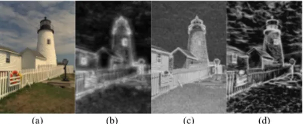
Fig. 4. Illustration of the comparison of ICM extracted from IWSSIM, VIF, or IWPSNR and the PCM extracted from FSIM and a representative saliency map (i.e., Torralba) for one of the source images in the LIVE database. (a) Original image. (b) Saliency map. (c) ICM. (d) PCM.

nonexistent or even negative (i.e., the averagedCC is−1.1% for IWSSIM, −0.1% for FSIM, 0.1% for VIF, and 0.2% for IWPSNR). Compared with such a marginal gain, adding com-putational saliency to other IQMs, such as UQI, yields a larger amount of performance gain (e.g., the averagedCC is 3.6% for UQI). The difference in the performance gain between IQMs may be attributed to the fact that some IQMs already contain saliency aspects in their metric design but others do not. For example, IWSSIM, VIF, and IWPSNR incorporate the estimate of local information content, which is often applied as a relevant cue in saliency modeling [37]. Phase congruency, which is implemented in FSIM, manifests itself as a meaningful feature of visual saliency [76]. Fig. 4 shows the so-called information content map (ICM) (i.e., extracted from IWSSIM, VIF, or IWPSNR) and the phase congruency map (PCM) (i.e., extracted from FSIM) to a representative saliency map (i.e., Torralba). It clearly visualizes the similarity between ICM/PCM and the real saliency map; the Pearson CC is 0.72 between ICM and Torralba and 0.79 between PCM and Torralba. Similarly, JNBM and NBAM intrinsically bear saliency characteristics (e.g., contrast). As such, the relatively small gain obtained for the aforementioned IQMs is probably caused by the saturation effect in saliency-based optimization (i.e., the double inclusion of saliency).

Based on the observed trend, one may hypothesize that adding computational saliency produces a larger improvement for IQMs without built-in saliency than for IQMs that intrin-sically include saliency aspects. To validate this hypothesis, we perform a straightforward statistical test. On account of a normally distributed-dependent variable performance gain, a t-test is performed with two levels of the variable being the IQMs with built-in saliency (i.e., IWSSIM, VIF, FSIM, IWPSNR, NBAM, and JNBM) and the IQMs without (i.e., PSNR, UQI, SSIM, MSSIM, NPBM, and GBIM). The

t-test results (T -value =5.37, P <0.01 at 95% level) show that IQMs without built-in saliency (gain = 2.3%) receive on average statistically significantly higher performance gain than the IQMs with built-in saliency (gain =0.18%).

Since IQMs can also be characterized at a different aggregation level, using FR/NR as the classification variable, a practical question arises whether FR/NR has an impact on the performance gain, and if so, to what extent. To check such effect with a statistical analysis, a t-test is performed again in a similar way as described above, but with two new independent variables to substitute the variable with/without built-in saliency: 1) FR and 2) NR. The t-test results

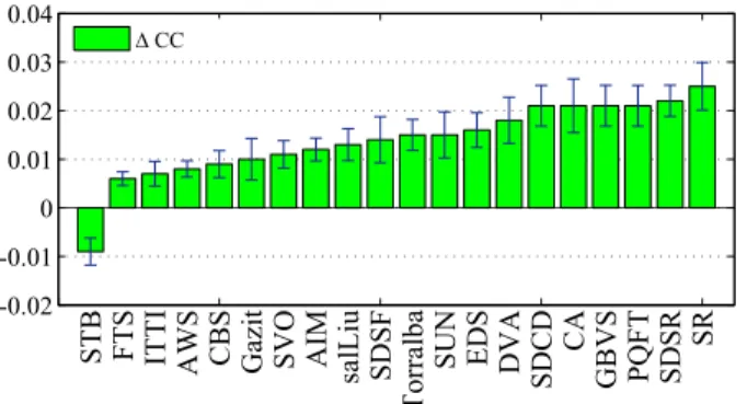
Fig. 5. Illustration of the rankings of the saliency models in terms of the overall performance gain (expressed by CC, averaged over all distortion types and over all IQMs where appropriate) between an IQM and its saliency-based version. Error bars: 95% confidence interval.

(T -value = 2.11, P < 0.05 at 95% level) show that overall NR IQMs (gain = 2.5%) obtain a statistically significantly larger amount of performance gain than FR IQMs (gain = 0.9%). This implies that applying computational saliency to an NR IQM has potential to significantly boost its reliability in an effective way.

B. Effect of Saliency Model Dependence

There is a significant difference in the performance gain between saliency models. Fig. 5 shows the order of saliency models in terms of the average performance gain that can be obtained by adding individual models to IQMs. A promising gain is found when adding SR (gain = 2.5%), SDSR (gain = 2.2%), PQFT (gain = 2.1%), GBVS (gain = 2.1%), CA (gain = 2.1%), and SDCD (gain =2.1%) to IQMs. The gain achieved for these models is fairly comparable with (but not necessarily statistically significantly better than) the gain of adding ground-truth HSM (gain = 2%) to IQMs. At the other extreme, STB (gain = − 0.9%) tends to deteriorate the performance of IQMs, and saliency models, such as FTS (gain = 0.6%), do not yield an evident profit for IQMs. Fig. 6 shows the saliency models sitting at the two extremes of performance gain: the most profitable models (i.e., SR, SDSR, PQFT, and GBVS) versus the least profitable models (i.e., STB and FTS). The comparison indicates that SR, SDSR, PQFT, and GBVS make a sufficiently clear distinction between the salient and nonsalient regions, which aligns with the appearance of HSM, as shown in Fig. 6. STB, which predicts the order in which the eyes move, often highlights the fixation locations (e.g., a certain portion of a cap) rather than salient regions (e.g., the entire cap). Adding such saliency to IQMs may result in an overestimation of localized distortions. The relatively lower performance gain obtained with FTS is possibly caused by the fact that it segments objects, which are sequentially labeled in a random order. As such, adding saliency in an IQM could randomly give more weight to artifacts in one object (e.g., the yellow cap) than that in another object (e.g., the red cap).

Since it is customary to classify saliency models into two categories, which are referred to as SOD and fixation prediction (FP), we check whether and to what extent this categorical variable affects the performance gain. Based on

reveal that there is no significant difference in performance gain between these two categories. This suggests that the classification of saliency models to SOD and FP does not have direct implications for the trend of changes in performance gain of IQMs.

C. Effect of Distortion Type Dependence

On average, the distortion type has a statistically significant effect on the performance gain, with the order, as shown in Fig. 7. It shows that GBLUR (gain = 2.4%) profits most from adding computational saliency in IQMs, followed by FF (gain = 1.4%), JPEG (gain = 1.3%), JP2K (gain = 0.7%), and finally WN (gain = 0%). Such variation in performance gain may be attributed to the intrinsic differences in perceptual characteristics between individual distortion types. In the case of an image degraded with WN, as shown in Fig. 8(a), artifacts tend to be uniformly distributed over the entire image. At low quality, the distraction power of the (uniformly distributed) annoying artifacts is so strong that it may mask the effect of the natural scene saliency. As such, directly weighting the DM with saliency intrinsically underestimates the annoyance of the artifacts in the back-ground, and their impact on the quality judgement. This case may eventually offset any possible increase in performance and, as a consequence, may explain the overall nonexisting performance gain.

The promising performance gain obtained for GBLUR may be attributed to two possible causes. First, in the par-ticular case of images distorted with both unintended blur (e.g., on a high-quality foreground object) and intended blur (e.g., in the intentionally blurred background to increase the field of depth) [77], IQMs often confuse these two types of blur and process them in the same way. Adding saliency hap-pens to circumvent such confusion by reducing the importance of blur in the background, and as such might improve the over-all prediction performance of an IQM. Second, blur is predom-inantly perceived around strong edges in an image [58]; the addition of saliency effectively accounts for this perception by eliminating regions (e.g., the background) that are perceptually irrelevant to blur, and consequently may enhance the reliability of an IQM for blur assessment. To further confirm whether adding saliency indeed preserves the perceptually relevant regions for blur, we first rigorously partition an image into blur-relevant (i.e., strong-edge positions) and blur-irrelevant (i.e., nonstrong-edge positions) regions, and then compare the saliency residing in the relevant regions to that in the irrelevant regions. Fig. 9 shows the comparison of the average saliency in the blur-relevant and blur-irrelevant regions, for the 29 source images of the LIVE database. It demonstrates that including saliency intrinsically retains the regions that are perceptually more relevant to perceived blur, and this explains the improvement of an IQM in assessing GBLUR.

Fig. 6. Illustration of the saliency maps as the output of the least profitable saliency models and the most profitable saliency models for IQMs. The original image is taken from the LIVE database.

Fig. 7. Illustration of the ranking in terms of the overall performance gain (expressed by CC, averaged over all IQMs and over all saliency models where appropriate) between an IQM and its saliency based version, when assessing WN, JP2K, JPEG, FF, and GBLUR. Error bars: 95% confidence interval.

Fig. 8. Illustration of an image distorted with WN and its measured natural scene saliency and local distortions. (a) WN distorted image extracted from LIVE database. (b) Saliency map (i.e., Torralba) based on the original image of (a) in the LIVE database. (c) DM of (a) calculated by an IQM (i.e., SSIM).

Fig. 9. Illustration of the comparison of the averaged saliency residing in the blur-relevant regions (i.e., positions of the strong edges based on the Sobel edge detection) and blur-irrelevant regions (i.e., positions of the rest of the image) for the 29 source images of the LIVE database. The vertical axis indicates the averaged saliency value (based on the saliency map Torralba), and the horizontal axis indicates the 29 test images (the content and ordering of the images can be found in [28]).

In JPEG, JP2K, and FF, the perceived artifacts tend to be randomly distributed over the entire image due to the luminance and texture masking of the HVS [2]. This could further confuse the issue of assessing artifacts with the addition of saliency, despite the general effectiveness, as shown in Fig. 7. Fig. 10 shows a JPEG compressed image (bit rate = 0.4 b/pixel), and its corresponding saliency

Fig. 10. Illustration of a JPEG compressed image at a bit rate of 0.4 b/pixel, and its corresponding natural scene saliency as the output of a saliency model (i.e., Torralba). (a) JPEG compressed image (b) Saliency map (i.e., Torralba) based on the original image of (a).

(i.e., generated by Torralba [43]). Due to HVS masking, this image exhibits imperceptible artifacts in the salient regions (e.g., the lighthouse and rocks in the foreground), but relatively annoying artifacts in the nonsalient regions (e.g., the sky in the background). In such a demanding condition, directly combining the measured distortions with saliency to a large extent overlooks the impact of the background artifacts on the overall quality. In view of this, we may speculate such type of images may not profit from adding saliency in IQMs, which also implies that the performance gain obtained so far for JPEG, JP2K, and FF may not be optimal amount. The overall positive gain, as shown in Fig. 7, however, can be explained by the fact that most of the images in the LIVE database exist of one of the following types: 1) images having visible artifacts uniformly distributed over the entire image and 2) images having the artifacts masked by the content in the less salient regions, but showing visible artifacts in the more salient regions. Obviously, for these two types of images, adding saliency is reasonably safe.

Also, as the speculation mentioned in [19] and [78], the observed trend that the amount of performance gain varies depending on the type of distortion may be associated with the performance of IQMs without saliency. For example, it may be more difficult to obtain a significant increase in performance by adding saliency when IQMs (without saliency) already achieve a high prediction performance for a given type of distortion. This phenomenon can be further revealed by checking the correlation between the performance (without saliency) and the performance gain (with the addition of saliency) of IQMs for WN, JP2G, JPEG, FF, and GBLUR. The Pearson CC is −0.71 and indicates that the higher the performance without saliency, the more the gain is limited by adding saliency.

V. INTEGRATINGCOMPUTATIONALSALIENCY INIQMs: RECIPE FORSUCCESS

This section summarizes the above-mentioned exhaustive evaluation, and provides guidance on good practices in the application of computational saliency in IQMs.

gain varies among individual combinations of the two variables: a) saliency models and b) IQMs. This variation directs the real-world applications of saliency-based IQMs, in which implementation choices are often confronted with a tradeoff between performance and computational efficiency. The measured gain for a given combination can be used as a reference to assist in making decisions about how to balance the performance gain of a saliency-based IQM against the additional costs needed for the saliency modeling and inclusion. 2) To decide upon whether a saliency model is in a

position to deliver an optimized performance gain for IQMs, it is essential to check the overall gain that can be actually obtained by adding this saliency model in the state-of-the-art IQMs. We found a threshold value in the overall gain, i.e., 2%, above which the effectiveness of a saliency model, such as SR, SDSR, PQFT, GBVS, CA, and SDCD, is comparable with that of the eye-tracking data and thus is considered to be an optimized amount. Such profit achieved by a saliency model, surprisingly, has no direct relevance to its measured prediction accuracy of human fixations. Moreover, the customary classification of saliency models (i.e., SOD and FP) is not informative on the trend of changes in performance gain; the most profitable models and the least profitable models can be found in both classes. 3) When it comes to the issues relating to the IQM

dependence of the performance improvement, care should be taken to make a distinction between the IQMs with and without built-in saliency aspects. Adding computational saliency to the former category intrinsically confuses the workings of saliency inclusion, and often produces a smattering of profit. The performance of the latter category of IQMs, however, can be boosted to a large degree with the addition of computational saliency. In terms of a different aggregation level, NR IQMs significantly profit more from including computational saliency than FR IQMs. 4) The effectiveness of applying saliency-based IQMs in

the assessment of different distortion types is subject to the perceptual characteristics of the distortions. The appearance of the perceived artifacts, such as their spatial distribution due to HVS masking, tends to influence the extent to which a certain image may profit from adding saliency to IQMs. Overall, we found that images degraded with GBLUR respond positively to the addition of saliency in IQMs, whereas saliency inclusion does not deliver added value when assessing the quality of images degraded with WN. In practice, it should, however, be mindful of the images distorted with localized artifacts, which may further confuse the operations of adding saliency in IQMs.

local saliency. This combination strategy is parameter free and therefore is universally applicable. More sophisticated combination strategies may further improve the added value of saliency inclusion in IQMs in more demanding conditions, but probably at the expense of their generality.

VI. CONCLUSION

In this paper, an exhaustive statistical evaluation is conducted to investigate the added value of including com-putational saliency in objective image quality assessment. The testbed comprises 20 best-known saliency models, 12 state-of-the-art FR and NR IQMs, and five image distortion types. It results in 880 possible combinations; each represents a case of performance gain of a saliency-based IQM over its original version when assessing the quality of images degraded with a given distortion type. Knowledge as the outcome of this paper is highly beneficial to the image quality community to have a better understanding of saliency modeling and inclusion in IQMs. Our findings are valuable to guide developers or users of IQMs to select or decide on appropriate saliency model for their specific application environments. The statis-tical evaluation also provides a thorough grounding for the quest of a more reliable saliency modeling in the context of image quality assessment.

REFERENCES

[1] W. Zhang and H. Liu. (2015). Toolbox: Integration of Visual Saliency

Models in Objective Image Quality Assessment. [Online]. Available:

https://sites.google.com/site/vaqatoolbox/

[2] Z. Wang and A. C. Bovik, Modern Image Quality Assessment. San Rafael, CA, USA: Morgan & Claypool, 2006.

[3] A. B. Watson, Digital Images and Human Vision. Cambridge, MA, USA: MIT Press, 1997.

[4] B. A. Wandell, Foundations of Vision. Sunderland, MA, USA: Sinauer Associates, 1995.

[5] W. S. Geisler and M. S. Banks, “Visual performance,” in Handbook of

Optics. New York, NY, USA: McGraw-Hill, 1995.

[6] A. B. Watson, G. Y. Yang, J. A. Solomon, and J. Villasenor, “Visibility of wavelet quantization noise,” IEEE Trans. Image Process., vol. 6, no. 8, pp. 1164–1175, Aug. 1997.

[7] S. J. Daly, “Visible differences predictor: An algorithm for the assess-ment of image fidelity,” Proc. SPIE, vol. 1666, pp. 2–15, Aug. 1992. [8] J. Lubin, “The use of psychophysical data and models in the analysis

of display system performance,” in Digital Images and Human Vision, A. B. Watson, Ed. Cambridge, MA, USA: MIT Press, 1993.

[9] A. B. Watson, “DCTune: A technique for visual optimization of DCT quantization matrices for individual images,” in 24th Soc. Inf. Dispaly

Dig. Tech. Papers, 1993, p. 946.

[10] J. Mannos and D. J. Sakrison, “The effects of a visual fidelity criterion of the encoding of images,” IEEE Trans. Inf. Theory, vol. 20, no. 4, pp. 525–536, Jul. 1974.

[11] Z. Wang, A. C. Bovik, H. R. Sheikh, and E. P. Simoncelli, “Image quality assessment: From error visibility to structural similarity,” IEEE

Trans. Image Process., vol. 13, no. 4, pp. 600–612, Apr. 2004.

[12] H. R. Sheikh and A. C. Bovik, “Image information and visual quality,”

IEEE Trans. Image Process., vol. 15, no. 2, pp. 430–444, Feb. 2006.

[13] H. R. Sheikh, A. C. Bovik, and L. Cormack, “No-reference quality assessment using natural scene statistics: JPEG2000,” IEEE Trans.

[14] L. Shao, L. Liu, and X. Li, “Feature learning for image classification via multiobjective genetic programming,” IEEE Trans. Neural Netw. Learn.

Syst., vol. 25, no. 7, pp. 1359–1371, Jul. 2014.

[15] F. Zhu and L. Shao, “Weakly-supervised cross-domain dictionary learn-ing for visual recognition,” Int. J. Comput. Vis., vol. 109, nos. 1–2, pp. 42–59, Aug. 2014.

[16] L. Shao, X. Zhen, D. Tao, and X. Li, “Spatio-temporal Laplacian pyramid coding for action recognition,” IEEE Trans. Cybern., vol. 44, no. 6, pp. 817–827, Jun. 2014.

[17] L. Shao, R. Yan, X. Li, and Y. Liu, “From heuristic optimization to dictionary learning: A review and comprehensive comparison of image denoising algorithms,” IEEE Trans. Cybern., vol. 44, no. 7, pp. 1001–1013, Jul. 2014.

[18] L. Shao, F. Zhu, and X. Li, “Transfer learning for visual categorization: A survey,” IEEE Trans. Neural Netw. Learn. Syst., vol. 26, no. 5, pp. 1019–1034, May 2015.

[19] H. Liu and I. Heynderickx, “Visual attention in objective image quality assessment: Based on eye-tracking data,” IEEE Trans. Circuits Syst.

Video Technol., vol. 21, no. 7, pp. 971–982, Jul. 2011.

[20] O. Le Meur, A. Ninassi, P. Le Callet, and D. Barba, “Overt visual attention for free-viewing and quality assessment tasks: Impact of the regions of interest on a video quality metric,” Signal Process., Image

Commun., vol. 25, no. 7, pp. 547–558, Aug. 2010.

[21] U. Engelke, H. Kaprykowsky, H. Zepernick, and P. Ndjiki-Nya, “Visual attention in quality assessment,” IEEE Signal Process. Mag., vol. 28, no. 6, pp. 50–59, Nov. 2011.

[22] H. Liu, U. Engelke, J. Wang, P. Le Callet, and I. Heynderickx, “How does image content affect the added value of visual attention in objective image quality assessment?” IEEE Signal Process. Lett., vol. 20, no. 4, pp. 355–358, Apr. 2013.

[23] X. Feng, T. Liu, D. Yang, and Y. Wang, “Saliency based objective quality assessment of decoded video affected by packet losses,” in Proc.

15th IEEE Int. Conf. Image Process., San Diego, CA, USA, Oct. 2008,

pp. 2560–2563.

[24] N. G. Sadaka, L. J. Karam, R. Ferzli, and G. P. Abousleman, “A no-reference perceptual image sharpness metric based on saliency-weighted foveal pooling,” in Proc. 15th IEEE Int. Conf. Image Process., San Diego, CA, USA, Oct. 2008, pp. 369–372.

[25] Q. Ma and L. Zhang, “Image quality assessment with visual attention,” in Proc. 15th Int. Conf. Pattern Recognit., Tampa, FL, USA, Dec. 2008, pp. 1–4.

[26] R. Barland and A. Saadane, “Blind quality metric using a percep-tual importance map for JPEG-20000 compressed images,” in Proc.

13th IEEE Int. Conf. Image Process., Atlanta, GA, USA, Oct. 2006,

pp. 2941–2944.

[27] D. Venkata Rao, N. Sudhakar, I. R. Babu, and L. P. Reddy, “Image quality assessment complemented with visual regions of interest,” in

Proc. Int. Conf. Comput., Theory Appl., Mar. 2007, pp. 681–687.

[28] H. R. Sheikh, Z. Wang, L. Cormack, and A. Bovik. Live Image Quality Assessment Database Release 2. [Online]. Available:

http://live.ece.utexas.edu/research/quality, accessed 2006.

[29] D. Walther and C. Koch, “Modeling attention to salient proto-objects,”

Neural Netw., vol. 19, no. 9, pp. 1395–1407, Nov. 2006.

[30] Z. Wang, E. P. Simoncelli, and A. C. Bovik, “Multiscale structural similarity for image quality assessment,” in Proc. 37th Asilomar Conf.

Signals, Syst. Comput., vol. 2. Nov. 2003, pp. 1398–1402.

[31] A. Borji, D. N. Sihite, and L. Itti, “Quantitative analysis of human-model agreement in visual saliency human-modeling: A comparative study,”

IEEE Trans. Image Process., vol. 22, no. 1, pp. 55–69, Jan. 2013.

[32] A. Borji, D. N. Sihite, and L. Itti, “Salient object detection: A bench-mark,” in Proc. 12th Eur. Conf. Comput. Vis., Florence, Italy, Oct. 2012, pp. 414–429.

[33] A. Borji, M.-M. Cheng, H. Jiang, and J. Li. (2014). “Salient object detection: A survey.” [Online]. Available: http://arxiv.org/abs/1411.5878 [34] A. Borji, M.-M. Cheng, H. Jiang, and J. Li. (2015). “Salient object detec-tion: A benchmark.” [Online]. Available: http://arxiv.org/abs/1501.02741 [35] Y. Fang, Z. Chen, W. Lin, and C.-W. Lin, “Saliency detection in the compressed domain for adaptive image retargeting,” IEEE Trans. Image

Process., vol. 21, no. 9, pp. 3888–3901, Sep. 2012.

[36] L. Itti, C. Koch, and E. Niebur, “A model of saliency-based visual attention for rapid scene analysis,” IEEE Trans. Pattern Anal. Mach.

Intell., vol. 20, no. 11, pp. 1254–1259, Nov. 1998.

[37] N. D. B. Bruce and J. K. Tsotsos, “Saliency, attention, and visual search: An information theoretic approach,” J. Vis., vol. 9, no. 3, p. 5, 2009.

[38] L. Zhang, M. H. Tong, T. K. Marks, H. Shan, and G. W. Cottrell, “SUN: A Bayesian framework for saliency using natural statistics,” J. Vis., vol. 8, no. 7, p. 32, 2008.

[39] X. Hou and L. Zhang, “Dynamic visual attention: Searching for coding length increments,” in Proc. 22th Conf. Adv. Neural Inf. Process. Syst., Vancouver, BC, Canada, Dec. 2008, pp. 681–688.

[40] J. Harel, C. Koch, and P. Perona, “Graph-based visual saliency,” in Proc.

20th Conf. Adv. Neural Inf. Process. Syst., Vancouver, BC, Canada,

Dec. 2006, pp. 545–552.

[41] T. Liu et al., “Learning to detect a salient object,” IEEE Trans. Pattern

Anal. Mach. Intell., vol. 33, no. 2, pp. 353–367, Feb. 2011.

[42] S. Goferman, L. Zelnik-Manor, and A. Tal, “Context-aware saliency detection,” IEEE Trans. Pattern Anal. Mach. Intell., vol. 34, no. 10, pp. 1915–1926, Oct. 2012.

[43] A. Torralba, “Modeling global scene factors in attention,” J. Opt. Soc.

Amer. A, vol. 20, no. 7, pp. 1407–1418, 2003.

[44] X. Hou and L. Zhang, “Saliency detection: A spectral residual approach,” in Proc. 20th IEEE Conf. Comput. Vis. Pattern Recognit., Minneapolis, MN, USA, Jun. 2007, pp. 1–8.

[45] C. Guo and L. Zhang, “A novel multiresolution spatiotemporal saliency detection model and its applications in image and video compression,”

IEEE Trans. Image Process., vol. 19, no. 1, pp. 185–198, Jan. 2010.

[46] R. Achanta, S. Hemami, F. Estrada, and S. Susstrunk, “Frequency-tuned salient region detection,” in Proc. 19th IEEE Conf. Comput. Vis. Pattern

Recognit., Feb. 2009, pp. 1597–1604.

[47] P. L. Rosin, “A simple method for detecting salient regions,” Pattern

Recognit., vol. 42, no. 11, pp. 2363–2371, Nov. 2009.

[48] M. Holtzman-Gazit, L. Zelnik-Manor, and I. Yavneh, “Salient edges: A multi scale approach,” in Proc. 11th Eur. Conf. Comput. Vis., Sep. 2010, pp. 1–14.

[49] H. Jiang, J. Wang, Z. Yuan, T. Liu, N. Zheng, and S. Li, “Automatic salient object segmentation based on context and shape prior,” in Proc.

22th Brit. Mach. Vis. Conf., Dundee, U.K., Sep. 2011, p. 7.

[50] A. Garcia-Diaz, X. R. Fdez-Vidal, X. M. Pardo, and R. Dosil, “Saliency from hierarchical adaptation through decorrelation and variance normal-ization,” Image Vis. Comput., vol. 30, no. 1, pp. 51–64, Jan. 2012. [51] H. J. Seo and P. Milanfar, “Static and space-time visual saliency

detection by self-resemblance,” J. Vis., vol. 9, no. 12, p. 15, 2009. [52] J. Li et al., “Saliency detection based on frequency and spatial domain

analyses,” in Proc. 22th Brit. Mach. Vis. Conf., Dundee, U.K., Sep. 2011, pp. 86.1–86.11.

[53] K.-Y. Chang, T.-L. Liu, H.-T. Chen, and S.-H. Lai, “Fusing generic objectness and visual saliency for salient object detection,” in Proc. 14th

IEEE Int. Conf. Comput. Vis., Barcelona, Spain, Nov. 2011, pp. 914–921.

[54] Z. Wang and A. C. Bovik, “A universal image quality index,” IEEE

Signal Process. Lett., vol. 9, no. 3, pp. 81–84, Mar. 2002.

[55] Z. Wang and Q. Li, “Information content weighting for perceptual image quality assessment,” IEEE Trans. Image Process., vol. 20, no. 5, pp. 1185–1198, May 2011.

[56] L. Zhang, D. Zhang, and X. Mou, “FSIM: A feature similarity index for image quality assessment,” IEEE Trans. Image Process., vol. 20, no. 8, pp. 2378–2386, Aug. 2011.

[57] H. R. Wu and M. Yuen, “A generalized block-edge impairment met-ric for video coding,” IEEE Signal Process. Lett., vol. 4, no. 11, pp. 317–320, Nov. 1997.

[58] P. Marziliano, F. Dufaux, S. Winkler, and T. Ebrahimi, “A no-reference perceptual blur metric,” in Proc. 9th IEEE Int. Conf. Image Process., Rochester, NY, USA, Sep. 2002, pp. III-57–III-60.

[59] R. Ferzli and L. J. Karam, “A no-reference objective image sharpness metric based on the notion of just noticeable blur (JNB),” IEEE Trans.

Image Process., vol. 18, no. 4, pp. 717–728, Apr. 2009.

[60] R. Muijs and I. Kirenko, “A no-reference blocking artifact measure for adaptive video processing,” in Proc. 13th Eur. Signal Process. Conf., Antalya, Turkey, Sep. 2005, pp. 1–4.

[61] D. M. Chandler and S. S. Hemami, “VSNR: A wavelet-based visual signal-to-noise ratio for natural images,” IEEE Trans. Image Process., vol. 16, no. 9, pp. 2284–2298, Sep. 2007.

[62] E. C. Larson and D. M. Chandler, “Most apparent distortion: Full-reference image quality assessment and the role of strategy,” J. Electron.

Imag., vol. 19, no. 1, p. 011006, Jan. 2010.

[63] N. Damera-Venkata, T. D. Kite, W. S. Geisler, B. L. Evans, and A. C. Bovik, “Image quality assessment based on a degradation model,”

IEEE Trans. Image Process., vol. 9, no. 4, pp. 636–650, Apr. 2000.

[64] P. Le Callet and F. Autrusseau. (2005). Subjective Quality

Assess-ment IRCCyN/IVC Database. [Online]. Available:

[68] M. Dorr, T. Martinetz, K. R. Gegenfurtner, and E. Barth, “Variability of eye movements when viewing dynamic natural scenes,” J. Vis., vol. 10, no. 10, p. 28, 2010.

[69] Q. Zhao and C. Koch, “Learning visual saliency by combining feature maps in a nonlinear manner using AdaBoost,” J. Vis., vol. 12, no. 6, p. 22, 2012.

[70] A. K. Moorthy and A. C. Bovik, “Visual importance pooling for image quality assessment,” IEEE J. Sel. Topics Signal Process., vol. 3, no. 2, pp. 193–201, Apr. 2009.

[71] J. Redi, H. Liu, P. Gastaldo, R. Zunino, and I. Heynderickx, “How to apply spatial saliency into objective metrics for JPEG compressed images?” in Proc. 16th IEEE Int. Conf. Image Process., Cairo, Egypt, Nov. 2009, pp. 961–964.

[72] Video Quality Experts Group, “Final report from the video quality experts group on the validation of objective models of video quality assessment, phase II (FR-TV2),” VQEG, Tech. Rep., 2003.

[73] S. Winkler, “Vision models and quality metrics for image processing applications,” Ph.D. dissertation, Dept. Elect. Eng., Univ. Lausanne, Lausanne, Switzerland, 2000.

[74] H. R. Sheikh, M. F. Sabir, and A. C. Bovik, “A statistical evaluation of recent full reference image quality assessment algorithms,” IEEE Trans.

Image Process., vol. 15, no. 11, pp. 3440–3451, Nov. 2006.

[75] D. C. Montgomery, Applied Statistics and Probability for Engineers, 6th ed. New York, NY, USA: Wiley, 2013.

[76] L. Ma, J. Tian, and W. Yu, “Visual saliency detection in image using ant colony optimisation and local phase coherence,” Electron. Lett., vol. 46, no. 15, pp. 1066–1068, Jul. 2010.

[77] H. Liu, J. Wang, J. Redi, P. Le Callet, and I. Heynderickx, “An efficient no-reference metric for perceived blur,” in Proc. 3rd Eur. Workshop Vis.

Inf. Process., Paris, France, Jul. 2011, pp. 174–179.

[78] J. Redi, H. Liu, R. Zunino, and I. Heynderickx, “Interactions of visual attention and quality perception,” Proc. SPIE, vol. 7865, pp. 78650S-1–78650S-11, Jan. 2011.

Wei Zhang (S’14) received the B.S. and M.S. degrees from Xidian University, Xi’an, China, in 2011 and 2013, respectively. He is currently a Ph.D. student with the School of Computer Science and Informatics at Cardiff University, Cardiff, U.K.

His research interests include image analysis, video processing, and human visual perception.

Ali Borji (M’10) received the B.S. and M.S. degrees in computer engineering from the Petroleum Uni-versity of Technology, Tehran, Iran, in 2001, and Shiraz University, Shiraz, Iran, in 2004, respectively. He received the Ph.D. degree in computational neu-rosciences from the Institute for Studies in Funda-mental Sciences (IPM) in Tehran, in 2009.

He spent a year at the University of Bonn, Bonn, Germany, as a Research Assistant. He was a Post-Doctoral Scholar at iLab, University of Southern California, Los Angeles, CA, USA, from 2010 to 2014. He was an Assistant Professor at the University of Wisconsin, Milwau-kee, WI, USA, from 2014 to 2015. He is currently an Assistant Professor at the Centre for Research in Computer Vision at the University of Central Florida, Orlando, FL, USA. His research interests include computer vision, machine learning, and neurosciences with a particular emphasis on visual attention, visual search, active learning, scene and object recognition, and biologically plausible vision models.

research interests include image processing, coding, and quality assessment, computational vision and pattern analysis, multimedia communications, and biomedical signal processing.

Dr. Wang was a member of the IEEE Multimedia Signal Processing Technical Committee from 2013 to 2015. He was a recipient of the 2014 NSERC E.W.R. Steacie Memorial Fellowship Award, the 2013 IEEE Signal Processing Best Magazine Paper Award, the 2009 IEEE Signal Processing Society Best Paper Award, the 2009 Ontario Early Researcher Award, and the ICIP 2008 IBM Best Student Paper Award (as senior author). He served as an Associate Editor of the IEEE TRANSACTIONS ONIMAGEPROCESSING from 2009 to 2014, and the IEEE SIGNALPROCESSINGLETTERSfrom 2006 to 2010, and a Guest Editor of the IEEE JOURNAL OFSELECTEDTOPICS IN SIGNALPROCESSINGfrom 2013 to 2014 and 2007 to 2009, the EURASIP

Journal of Image and Video Processing from 2009 to 2010, and Signal, Image and Video Processing from 2011 to 2013. He has been an Associate Editor

of Pattern Recognition since 2006.

Patrick Le Callet (M’05–SM’14) received the M.Sc. and Ph.D. degrees in image processing from the Ecole Polytechnique de l’Universite de Nantes, Nantes, France.

He was with the Department of Electrical Engi-neering, Technical Institute of the University of Nantes, Nantes, as an Assistant Professor from 1997 to 1999 and a full-time Lecturer from 1999 to 2003. Since 2003, he teaches with the Department of Electrical Engineering and the Department of Com-puter Science, École Polytechnique de l’Universite de Nantes (Engineering School), where he is currently a Full Professor. Since 2006, he has been the Head of the Image and Video Communication Laboratory with CNRS IRCCyN, a group of more than 35 researchers. He is currently involved in research dealing with the application of human vision modeling in image and video processing. He has co-authored over 200 publications and communications and holds 13 international patents in his research topics. His current research interests include 3-D image and video quality assessment, watermarking techniques, and visual attention modeling and applications.

Prof. Le Callet served as an Associate Editor of several journals, such as the IEEE TRANSACTIONS ONIMAGEPROCESSING, the IEEE TRANSACTIONS ONCIRCUITSYSTEM ANDVIDEOTECHNOLOGY, the EURASIP Journal on

Image and Video Processing, and SPIE Electronic Imaging.

Hantao Liu (S’07–M’11) received the M.Sc. degree from the University of Edinburgh, Edinburgh, U.K., and the Ph.D. degree from the Delft University of Technology, Delft, The Netherlands, in 2005 and 2011, respectively.

He is currently an Assistant Professor with the School of Computer Science and informatics, Cardiff University, Cardiff, U.K. His research inter-ests include visual media quality assessment, visual attention modelling and applications, visual scene understanding, and medical image perception. Prof. Liu is currently serving for IEEE MMTC as the Chair of the Interest Group on Quality of Experience for Multimedia Communications.