series forecasts through linear programming. PhD
thesis, University of Nottingham.
Access from the University of Nottingham repository:
http://eprints.nottingham.ac.uk/12515/1/Apostolos_Panagiotopoulos_Thesis.pdf
Copyright and reuse:
The Nottingham ePrints service makes this work by researchers of the University of Nottingham available open access under the following conditions.
· Copyright and all moral rights to the version of the paper presented here belong to the individual author(s) and/or other copyright owners.
· To the extent reasonable and practicable the material made available in Nottingham ePrints has been checked for eligibility before being made available.
· Copies of full items can be used for personal research or study, educational, or not-for-profit purposes without prior permission or charge provided that the authors, title and full bibliographic details are credited, a hyperlink and/or URL is given for the original metadata page and the content is not changed in any way.
· Quotations or similar reproductions must be sufficiently acknowledged.
Please see our full end user licence at:
http://eprints.nottingham.ac.uk/end_user_agreement.pdf A note on versions:
The version presented here may differ from the published version or from the version of record. If you wish to cite this item you are advised to consult the publisher’s version. Please see the repository url above for details on accessing the published version and note that access may require a subscription.
OPTIMISING TIME SERIES FORECASTS THROUGH
LINEAR PROGRAMMING
Apostolos Panagiotopoulos, MSc
Thesis submitted to the University of Nottingham for the
degree of Doctor of Philosophy
i To the memory of my beloved aunt Fotini Schiza and my fraternal friend Georgios Brillakis
ii
ABSTRACT
This study explores the usage of linear programming (LP) as a tool to optimise the parameters of time series forecasting models. LP is the most well-known tool in the field of operational research and it has been used for a wide range of optimisation problems. Nonetheless, there are very few applications in forecasting and all of them are limited to causal modelling. The rationale behind this study is that time series forecasting problems can be treated as optimisation problems, where the objective is to minimise the forecasting error.
The research topic is very interesting from a theoretical and mathematical prospective. LP is a very strong tool but simple to use; hence, an LP-based approach will give to forecasters the opportunity to do accurate forecasts quickly and easily. In addition, the flexibility of LP can help analysts to deal with situations that other methods cannot deal with.
The study consists of five parts where the parameters of forecasting models are estimated by using LP to minimise one or more accuracy (error) indices (sum of absolute deviations – SAD, sum of absolute percentage errors – SAPE, maximum absolute deviation – MaxAD, absolute differences between deviations – ADBD and absolute differences between percentage deviations – ADBPD). In order to test the accuracy of the approaches two samples of series from the M3 competition are used and the results are compared with traditional techniques that are found in the literature.
In the first part simple LP is used to estimate the parameters of autoregressive based forecasting models by minimising one error index and they are compared with the method of the ordinary least squares (OLS minimises the sum of squared errors, SSE). The experiments show that the decision maker has to choose the best optimisation objective according to the characteristic of the series. In the second part, goal programming (GP) formulations are applied to similar models by minimising a combination of two accuracy indices. The experiments show that goal programming improves the performance of the single objective approaches.
In the third part, several constraints to the initial simple LP and GP formulations are added to improve their performance on series with high randomness and their accuracy is compared with techniques that perform well on these series. The additional constraints improve the results and outperform all the other techniques. In the fourth part, simple LP and GP are used to combine forecasts. Eight simple individual techniques are combined and LP is compared with five traditional combination methods. The LP combinations outperform the other methods according to several
iii performance indices. Finally, LP is used to estimate the parameters of autoregressive based models with optimisation objectives to minimise forecasting cost and it is compared them with the OLS. The experiments show that LP approaches perform better in terms of cost.
The research shows that LP is a very useful tool that can be used to make accurate time series forecasts, which can outperform the traditional approaches that are found in forecasting literature and in practise.
iv
ACKNOWLEDGMENTS
There are several people I wish to thank for their support for the period of my doctoral studies. I would like to distinguish my supervisor Dr Luc Muyldermans and my uncle and godfather Apostolos Schizas. I am very appreciative to them because without the contribution of Luc this effort would have never been completed and without the contribution of Apostolos it would have never begun. Closing, I would like to express my gratefulness to my partner Georgia Latsi for being so supportive during the last year.
v
CONTENTS
ABSTRACT ... II ACKNOWLEDGMENTS ... IV CONTENTS... V LIST OF FIGURES ... VII
1 INTRODUCTION ... 1
1.1 RESEARCHSCOPEANDOBJECTIVES ... 1
1.2 RESEARCHOUTLINE ... 3
2 CURRENT RESEARCH STATUS ... 6
2.1 INTRODUCTIONTOFORECASTING ... 6
2.2 FORECASTINGTECHNIQUES ... 8
2.2.1 Quantitative forecasting ... 8
2.2.2 Qualitative Forecasting ... 9
2.2.3 Other forecasting techniques ... 11
2.2.4 Judgmental adjustments of quantitative forecasts ... 13
2.3 FORECASTINGERROR ... 15
2.3.1 Measuring forecasting error ... 15
2.3.2 Cost of forecasting error ... 20
2.4 TIMESERIESANALYSIS ... 21
2.4.1 Decomposition ... 21
2.4.2 Time series forecasting techniques ... 23
2.4.3 The Box-Jenkins methodology for ARIMA models ... 26
2.4.4 ARIMA extensions ... 30
2.5 COMBINEDFORECASTING ... 31
2.6 MATHEMATICALPROGRAMMINGFORFORECASTING ... 35
2.6.1 Mathematical programming in statistics ... 35
2.6.2 Mathematical programming for estimating the parameters of forecasting models... 40
2.6.3 Mathematical programming for combining forecasts ... 42
2.6.4 Discussion ... 45
2.7 THEFORECASTINGCOMPETITIONSANDTHEFUTUREOFFORECASTINGRESEARCH . 46 2.7.1 The M-Competitions ... 46
2.7.2 The NN Competitions ... 48
2.7.3 The future of forecasting research ... 48
2.8 CONCLUSION ... 50
3 RESEARCH METHODOLOGY ... 51
3.1 DEVELOPMENT ... 51
3.2 DATASELECTIONANDANALYSIS ... 51
3.3 TESTING,COMPARISONANDEVALUATION ... 66
3.3.1 Testing ... 66
3.3.2 Comparison and evaluation ... 67
3.4 CONCLUSION ... 73
4 OPTIMISING AUTOREGRESSIVE BASED FORECASTS ... 74
4.1 SIMPLEOBJECTIVEMODELS:INITIALFORMULATION ... 74
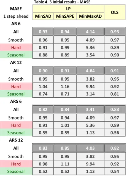
4.2 FIRSTRESULTS ... 80
4.3 INGNORINGTHEFIRST S+M-1DATAPOINTSINTHEOBJECTIVEFUNCTION ... 83
vi
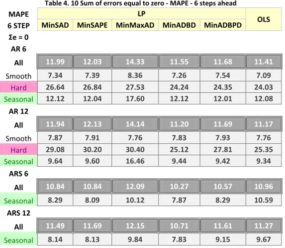
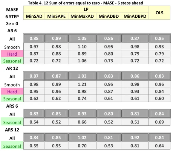
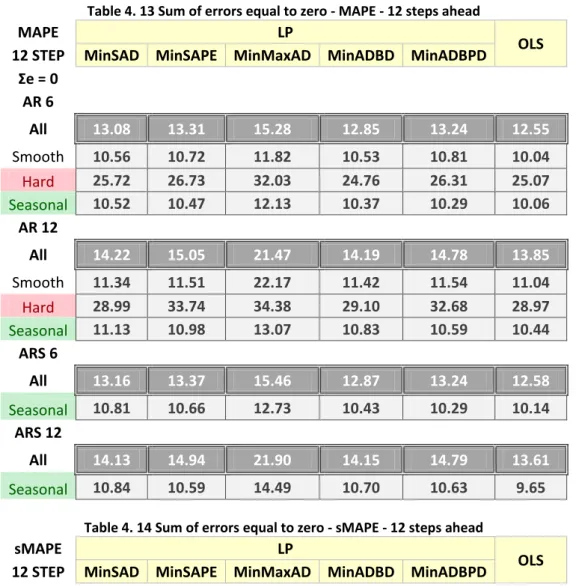
4.5 SUMOFERRORSEQUALTOZERO ... 87
4.6 RESULTS:SUMOFERRORSEQUALTOZERO ... 90
4.7 SUMOFPERCENTAGEERRORSEQUALTOZERO ... 97
4.8 CONCLUSIONS ... 104
5 GOAL PROGRAMMING FOR TIME SERIES FORECASTING ... 106
5.1 PRE-EMPTIVEGOALPROGRAMMING ... 106
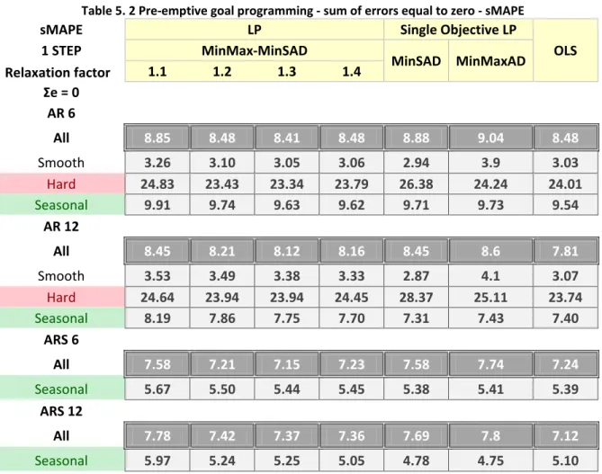
5.2 RESULTS:PREEMPTIVEGOALPROGRAMMING ... 108
5.3 WEIGHTEDGOALPROGRAMMING ... 113
5.4 WGPRESULTS:SUMOFERRORSEQUALTOZERO ... 114
5.5 WGPRESULTS:SUMOFPERCENTAGEERRORSEQUALTOZERO ... 121
5.6 CONCLUSIONS ... 127
6 LINEAR PROGRAMMING FOR FORECASTING SERIES WITH HIGH VARIABILITY... 129
6.1 APPROACHES ... 129
6.2 TESTS ... 130
6.3 RESULTS:SUMOFERRORSEQUALTOZERO ... 135
6.4 RESULTS:SUMOFPERCENTAGEERRORSEQUALTOZERO ... 140
6.5 CONCLUSION ... 145
7 LINEAR PROGRAMMING FOR COMBINED FORECASTING ... 147
7.1 SINGLEOBJECTIVEANDAVERAGELINEARPROGRAMMING ... 147
7.2 TESTS ... 149
7.3 FIRSTRESULTS ... 150
7.4 WEIGHTEDGOALPROGRAMMING ... 157
7.5 RESULTS ... 158
7.6 CONCLUSION ... 160
8 MINIMISING FORECASTING COST ... 162
8.1 COSTRELATIONSHIPINTHEOBJECTIVEFUNCTION ... 162
8.2 COSTRELATIONSHIPINTHECONSTRAINTS ... 164
8.3 RESULTS ... 166
8.4 CONCLUSIONS ... 171
9 CONCLUSION ... 173
9.1 SUMMARY ... 173
9.2 IMPLICATIONSFORFORECASTINGTHEORY ... 174
9.3 LIMITATIONS ... 175
9.4 RECOMMENDATIONSFORFURTHERRESEARCH ... 176
10 APPENDIX ... 178
10.1 SIMPLELP ... 178
10.2 WEIGHTEDGOALPROGRAMMING ... 181
10.3 CONCLUSION ... 184
vii
LIST OF FIGURES
Figure 2. 1 The most common forecasting techniques and their interactions ... 13
Figure 2. 2 Time series patterns ... 23
Figure 2. 3 The Box-Jenkins ARIMA methodology ... 30
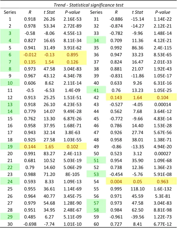
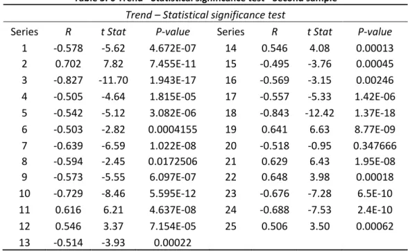
Figure 3. 1 Series with seasonality ... 56
Figure 3. 2 Autocorrelation graph: Series with seasonality ... 56
Figure 3. 3 Series with strong trend ... 57
Figure 3. 4 Autocorrelation graph: Series with trend ... 58
Figure 3. 5 Series with indication of high variability ... 58
Figure 3. 6 Autocorrelation graph: Series with indication of high variability ... 59
Figure 3. 7 Series with smoothed trend ... 59
Figure 3. 8 Series before the trend and seasonal adjustment ... 61
Figure 3. 9 Seasonal and trend adjusted series ... 62
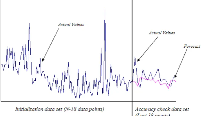
Figure 3. 10 The out of sample accuracy check ... 67
Figure 4. 1 Performance of an approach with the first s+m-1 point in the objective function ... 83
Figure 6. 1 Performance of an approach on a hard series on the training set and test set ... 129
Figure 6. 2 Performance of MA of order 1 - 12 ... 131
Figure 6. 3 Performance of WMA of order 1 - 12 ... 131
Figure 6. 4 Performance of SES with factor 0 - 1 ... 132
Figure 6. 5 Performance of Holt's with factors 0 - 1, 0 - 1 ... 132
Figure 7. 1 Number of times each individual technique gives the best results ... 152
Figure 7. 2 Number of times each individual technique gives the worst results ... 152
Figure 8. 1 Cost performance (all series) ... 169
Figure 8. 2 Cost performance (smooth series) ... 170
Figure 8. 3 Cost performance (hard series) ... 170
Figure 8. 4 Cost performance (seasonal series) ... 171
1
1
INTRODUCTION
Linear programming (LP) is the most well-known tool in the field of operational research. Since the formulation of the first LP problems by Leonid Kantorovich in 1939 (Kantorovich, 1960) and the development of the simplex algorithm by George B. Dantzig in 1947 (Dantzig, 2002), linear programming has been used in a wide range of optimisation problems that are found in business and management, such as transportation routing, project planning, production planning, supply chain management and portfolio optimisation.
Forecasting is a vital managerial activity as it is the first stage of every planning procedure. This research focuses on applying linear programming to solve forecasting problems. The main idea behind the study is that forecasting problems can be treated as optimisation problems, where the objective is to minimise the forecasting error.
1.1 RESEARCH SCOPE AND OBJECTIVES
The aim of the study is to examine the application of linear programming as a tool to estimate the parameters of time series forecasting models. The research compares the performance of the LP-based approaches with the traditional statistical tools that are found in the literature, specifies the advantages and the disadvantages of the former and concludes the cases, where they should be preferred.
The rationale for this topic is that it is very interesting from a theoretical and mathematical prospective. The topic rather focuses on the advancement of scientific knowledge about forecasting and it is not an actual forecasting application for business. However, LP is a very strong tool but simple to understand and to use; thus, if LP-based approaches are shown to be more or as accurate as the traditional methods it will give to forecasters the opportunity to do accurate forecasts quickly and easily.
The purpose of the research is explorative, because it tests the implementation of an idea that already exists. There is important research on the use of linear programming and optimisation as a tool for solving statistical problems, with a wide area of applications (e.g. descriminant analysis). However, applications of the former for optimising forecasts have not been investigated in detail and they are limited to causal forecasting applications (Trapp, 1986, Soliman et al. 1997). In addition,
2 the performance of LP-based approaches has neither been tested nor compared with traditional methods. Linear programming is a flexible tool that can exceed many limitations of the latter. This research aims to test the performance of LP-based approaches as an alternative and also to use it for solving problems that traditional statistical tools cannot deal with. The objectives of the study are to answer the following five questions and as a result to develop insights into the main aim:
I. How does linear programming perform in estimating the parameters of autoregressive based forecasting models? The traditional tool for the estimation of an autoregressive equation is the ordinary least squares method, which minimises the Sum of Squared Errors (SSE). LP gives the opportunity to minimise different accuracy indices, such as the Sum of Absolute Errors (SAD) and the Sum of Absolute Percentage Errors (SAPE). Thus, an LP approach will show how other indices perform compared with the SSE and in what situations they should be preferred.
II. “The performance of a technique may differ according to different accuracy measures” (Makridakis et al. 1984). Traditional tools aim to optimise one accuracy index (e.g. the least squares method minimises only the SSE). LP, in contrast with other techniques, can be applied for multi-objective optimisation (e.g. goal programming). Can linear goal programming be used to minimise two or more accuracy indices (e.g. SAD, Maximum Absolute Deviation - MaxAD) instead of only one? The study will show its performance and compare multi-objective and single objective LP optimisation methods.
III. One of the outcomes of past research (e.g Makridakis et. al, 1984) was that simple techniques, like moving average and exponential smoothing outperform more sophisticated techniques in series with high randomness. Can the flexibility of the linear programming approaches be exploited to improve the performance on series with high randomness? If yes, how does it perform compared with simpler techniques?
IV. Linear programming was suggested as a combination forecasting technique (Reeves and Lawrence 1982). Nevertheless, comparison with other methods to develop a good combination of forecasts (e.g. simple average, inverse proportion) is not available in the literature. How does linear programming perform as a tool for combining forecasts? LP guarantees the optimal combination between all the available forecasts, according to a preselected optimisation criterion (e.g. SAD). The study will show how LP models for combined forecasting perform compared with individual as well as traditional combination methods.
3 V. “Situations where the cost of overestimation differs from this of underestimation are very
common” (Newbold and Bos, 1994). Can linear programming be used to minimise the total forecasting cost (instead of error) in case the costs of overestimation and underestimation are different? The results will demonstrate how a cost minimisation model performs compared with the more traditional accuracy optimisation models and a sensitivity analysis will show in which cases (differences between underestimation and overestimation cost) the results are significantly different.
The first, the second and the fourth questions aim to test the applicability of linear programming for estimating the parameters of forecasting models, while the other two focus on exploiting the flexibility of linear programming to overcome some of the limitations of traditional statistical methods.
The study belongs in the scientific field of operational research/management science. Reisman and Kirschnick (1994, 1995) classify studies in this field in three categories, according to the research strategy and aim:
a. The first category includes studies of “meta-research” and research on the philosophy and history of OR.
b. Second is the “untested theory” that includes studies, which focus on theoretical OR topics, for example research on new OR tools, and are not real-world applications.
c. Third are the real-world applications that deal with real-world problems.
This study belongs to the second category, since it is neither research on the philosophy and history of OR, nor a real world managerial application. It is a pure theoretical OR study that focuses on a new LP-based methodology for estimating the parameters of well-known forecasting models.
1.2 RESEARCH OUTLINE
The thesis’ outline is as follows: There is a review of the related literature of the area, then the methodology of the study follows; I continue with the mathematical models and the results of the experiments and I finish with several conclusions. The structure of the thesis is the following.
Chapter 2 presents what is known in the field so far and it consists of seven parts. First is an introduction to forecasting, followed by a general review of the types of forecasting techniques. The
4 third part talks about the forecasting error. As the study is on time series forecasting the fourth part is more specific on time series analysis and forecasting techniques. Part five focuses on the field of combining forecasts. Part six is a review of the mathematical programming approaches for forecasting. The last part talks about seven forecasting competitions (M Competitions and NN Competitions) with objective to investigate how different techniques differ from each other and how forecasters can be able to make practical choices (Makridakis et al. 1984) and the future of forecasting research.
The methodology of the research can be found in Chapter 3. First is the development where I talk about the linear programming formulations. Second is the data, where I talk about the selection of the series for testing the techniques, the statistical analysis of them and their decomposition. The last part is the methodology of testing the forecasts, the comparison with traditional techniques found in the literature and the evaluation of the whole process.
The next five chapters aim to answer the five research questions respectively. In Chapter 4 simple LP is used to develop and optimise autoregressive based forecasting models. I estimate the coefficients of simple autoregressive models (AR) and autoregressive models with additive seasonality (ARS) by minimising SAD, SAPE, MaxAD, the Absolute Difference between Deviations (ADBD), and the Absolute Percentage Difference between Deviations (ADBPD). The accuracy of the LP based approaches is compared with the Ordinary Least Squares (OLS) method (minimising the Sum of Squared Errors). The study is mainly focused on this specific ARIMA (d,0,0) models due to the limitations of the LP. Only autoregressive models can be formulated as linear programs and the above minimisation objectives can follow a linear structure.
In Chapter 5 Linear Goal Programming formulations are applied to estimate the parameters of the same models. MinSum and MinMax pre-emptive and weighted goal programming is used (the latter is a relaxation of the former) to minimise both the SAD and the MaxAD. The results are compared with the OLS and the single objective approaches from Chapter 4.
Chapter 6 presents how the flexibility of LP can be exploited to improve the accuracy of autoregressive based forecasts on time series with high level variability and low predictability. I use all the simple LP and weighted goal programming models from Chapters 4 and 5 and I run experiments with additional constraints on a data set of series with high variability. The accuracy of the new approaches is compared with five traditional techniques, where the literature shows that they perform well in these cases.
5 In Chapter 7 I explore the use of LP as a tool to combine forecasts. I use simple LP and weighted goal programming. The former estimates the weights of several models by minimising the SAD, the SAPE and the MaxAD, whereas the latter minimises both the SAD and the MaxAD. The models combine eight individual forecasting techniques and we compare their accuracy with five other traditional combination methods.
Finally, in Chapter 8 I explore cases where the cost of the underestimation forecasting error differs from the overestimation cost. I apply simple LP methods to minimise the forecasting cost, instead of the error, or I use the simple LP methods from Chapter 4 adding the cost relationship of the underestimation and overestimation errors as a constraint. Experiments for five different cost relations are run and the approaches are compared with the OLS in terms of accuracy and cost. The approaches are limited on cases where the cost is a linear function to the forecasting error due to the LP limitations. The thesis finishes with several conclusions and recommendations for further research.
6
2
CURRENT RESEARCH STATUS
This chapter is a discussion of what is already known in the field. There is a general introduction to forecasting, where the distinctions between qualitative and quantitative forecasting and between causal and time series methods are presented. An analysis on the forecasting error (measurement methods and cost) follows. The next section focuses on time series analysis. There is a discussion about time series decomposition, the most common time series forecasting techniques and the Box-Jenkins methodology. Furthermore, there is a review of the area of combined forecasting. Subsequently, the chapter focuses on mathematical programming applications for forecasting. I present what has been done so far and I identify the research gaps that this study aims to cover. The chapter closes with a review of the forecasting competitions and the future of forecasting research.
2.1 INTRODUCTION TO FORECASTING
According to Armstrong (2001) forecasting is defined as the prediction of an actual value in a future time period. Makridakis et al. (1998) state that forecasting supplies information of what may occur in the future. Thus, it is used to estimate when an event is probable to happen so that proper action can be taken.
Forecasting in business practice is the basis every planning process; hence, it affects decisions and activities throughout an organisation. Examples of using forecasts in different areas of business practice are:
Accounting: Estimation of new product cost and cash flow management.
Finance: Time and amount of funding needs, budgeting, investment selection, credit scoring, credit risk management.
Human resources: recruitment needs, layoff planning.
Marketing: Pricing, placing and promotion, market entrance, competition strategies, direct marketing.
Operations: Inventory planning, capacity planning, supply-chain planning, work scheduling, production planning.
7 Information systems: systems revision.
R&D and design: New products and services introduction, technological progress.
Strategic management: Competition, economic conditions, new markets, goals planning.
According to Stevenson (2005) there are two applications of business forecasting. The first is to help the decision maker to plan the system and the second to plan the use of the system. Planning the system normally involves long-range plans such as product design, facilities layout, procurement of new equipment and location. On the other hand, planning the use of the system has to do with short and intermediate-range planning, such as inventory and workforce planning, work scheduling and budgeting.
In order to develop a forecast, the decision maker has to follow several steps. The number of steps varies, but, most researchers (e.g. Armstrong, 2001, Stevenson, 2005) agree on the following six:
1. Determination of the purpose of the forecast: That is the use and the objectives of the forecast. This will indicate the necessary accuracy level, the amount of resources that should be committed (people, computer time, money) and the cost of the forecasting error.
2. Specify the time horizon: A forecast may be long-range, intermediate-range or short-range, according to the forecasting purpose.
3. Method selection.
4. Data gathering and analysis: The data sources may be internal records (e.g. sales, demand, costs, stock control data, accounting data), external records (e.g. online data, government sources, periodicals and journals). Some data may not be available.
5. Make the forecast.
6. Monitor the forecast: Monitoring determines the performance of the forecast. If the forecast is not satisfactory, the decision maker has to re-examine the method, the data, the time horizon or even the purpose of the forecast. Then, (s)he has to start the process again from the corresponding step.
It is clear that forecasting is the starting point for various business decisions. The better an organisation’s forecasts are, the more it is ready to utilize potential prospects and decrease prospective risks. Thus, forecasters should be very keen in selecting the most appropriate techniques
8 and maintain their information sources up to date in order to keep the accuracy of their forecasts high.
2.2 FORECASTING TECHNIQUES
Forecasting techniques are classified in two categories: quantitative and qualitative (Makridakis et al., 1998 and Armstrong, 2001). They can also be found in the literature as objective and subjective, respectively (Nahmias, 2005). According to Makridakis et al. (1998) quantitative forecasting can be applied under three conditions:
1. Quantitative information availability about the past
2. This information can be expressed in numerical data.
3. Assumption of continuity, which is the statement that characteristics of the past patterns will continue in the future.
On the other hand, qualitative forecasting is applied in case of lack of quantitative information, but sufficient qualitative knowledge and experience exists. Finally, when neither quantitative information nor qualitative knowledge is available a satisfactory forecast cannot be performed.
Both quantitative and qualitative techniques differ extensively in accuracy, cost and complexity. Qualitative techniques, in general, are applied for longer term forecasting. Nonetheless, it is common for both methods to be combined. In practice, Sanders and Manrodt (2003) found significant differences in accuracy between companies that focus on only one of the above methods: organisations focusing on quantitative techniques tend to obtain better forecasts. However, the authors conclude that judgmental forecasting focused firms operate in more uncertain environments, which may explain the higher forecasting error.
2.2.1 Quantitative forecasting
Quantitative techniques are divided in two categories: explanatory (causal) models and time series models. The first category investigates the cause and effect relationship between the forecasted variable and one or more independent variables. Time series models predict the future value of a variable based upon its past values without attempting to estimate the external factors that affect this behaviour.
9 Specifically, explanatory forecasting is based on models in which the predicted value is related to various explanatory variables based on a specified theory (Armstrong, 2001). “The purpose of explanatory models is to discover the form of the relationship and use it to forecast future values of the forecast variable” (Makridakis et al., 1998).
The most common causal forecasting techniques are variations of linear and non-linear (e.g. logistic) simple and multiple regression models, where the dependent variable is the forecasted value and the independent variables are exogenous to this value. If Y is the dependent variable and X1, X2, X3,……, XNare the N independent variables, then:
(
X
X
X
X
N)
f
Y
=
1,
2,
3,....,
(2. 1)Econometric models are defined as a special category of regression models in which the relationship between dependent and independent variables is linear. The most common ways for the estimation of the parameters of regression based models are the least squares and the maximum likelihood method (Makridakis et al., 1998). Nevertheless, in case of more complicated non-linear relationships, more sophisticated estimation techniques can be used, like Bayesian networks or artificial neural networks.
On the other hand, time series forecasting is set from the theory that the history of incidences over time can be used to forecast the future. Thus, time series forecasting techniques are based on the concept of recognising a pattern that exists in a series. This study is focused on time series forecasting; hence, an extended review on time series analysis and techniques will follow.
2.2.2 Qualitative Forecasting
As it was mentioned above, qualitative techniques do not require numerical information, but their outcomes are based on the judgment and accumulated knowledge of “specially trained people” (Makridakis et al., 1998). Even if the forecasting research and practice has proved that quantitative forecasting is more accurate, qualitative forecasting is widely applied in business practice, especially in situations where no past information is available, or it cannot be quantified. The most common qualitative methods are presented in the following table.
10 Table 2. 1 Qualitative forecasting techniques
Technique Description
Grass Roots
Forecasters gather information from the executives and personnel (e.g. workers) who are at the lowest place of the hierarchy and usually closer to the forecasting problem. They use that information as a basis for judgmental forecasting.
Market Research
It is mainly used for long term market forecasting. The input is collected data from many ways, such as surveys, interviews and salesmen opinions.
Panel Consensus Free open discussion of an idea at meetings. All participants have the
right to express their ideas about the future (Galbraith et al. 2010).
Historical Analogy It is based on finding analogies with similar situations of the past and
identifying historical patterns (Dortmans and Eiffe, 2004).
Delphi Method
Group of experts responds to a questionnaire individually. Then a mediator gathers the results and formulates a new questionnaire that is resubmitted to the same group and the process is repeated. The repetition goes on until a forecast emerges (e.g. Kaynak et al., 1994, Lilja et al., 2011, Liu et al., 2010).
Sales Force Composite Sales executives forecast according to their daily interaction with
customers (Peterson, 1989 and 1993).
Unaided Judgment
This is a fast and inexpensive method, where a team of experts predict the result of current situations not aided by a formal forecasting technique and based only on their experience and possible data availability (Green, 2002). It has been proved very useful in cases where the expert has got good feedback about her/his forecasting accuracy. It is widely applied in the area of betting on sports.
Customer Surveys They are usually used to signal preferences and opinions about new
11
Cross – Impact Analysis
Forecasters submit their opinions about what is likely to influence the area of interest. It is common to be used in combination with Delphi method (Banuls and Turoff, 2011).
Scenario Writing
This technique is widely used for long term planning and strategic analysis. It is based on developing the most possible and probable scenarios about the future (e.g. Bunn and Salo, 1993, Kanama, 2010).
Economic Indicators
These are tracked across a time series. The economic description of the behaviour of the series identifies the situation and helps experts to develop judgmental forecasts (e.g. Fite et al., 2002, Ozyildirim et al. 2010).
Source: Armstrong (2001),Chase et al. (2006), Nahmias (2005) and Newbold and Bos (1994)
2.2.3 Other forecasting techniques
Academic research and business practice have produced several forecasting methods that are not classified according to the traditional quantitative – qualitative and time series – causal clustering. The majority of these techniques tend to follow a mixed quantitative/qualitative methodology and they aim to “balance data and judgment” (Bunn, 1996), without this being the rule. The most common are the following.
Simulation: Simulation is common to be usedwhen an analyst is asked to forecast the behaviour of a complex system over time. Simulation programs are designed to reflect the key aspects of a real situation (Pidd, 1998). The simulation method that is used depends on the characteristics of the system and the data availability. It usually combines both quantitative and qualitative elements and the balance between them differs according to the specific simulation method that is used. In business practice we can find applications of Monte Carlo (Pflaumer, 1988, Billio and Casarin, 2010), Discrete Event (Cheng and Duran, 2004), System Dynamics (Higuchi and Troutt, 2004, Wu et al., 2010), Role Playing (Green, 2002 and 2005) simulation and others. By running the simulation program under different starting conditions, a forecast for different situations is created (Nahmias, 2005).
12
Focus forecasting: The method is a rule based forecasting technique, where the analyst creates a simulation program under these rules. The program uses past data to measure how well the issued rules are performed (Chase et al., 2006).
Technical analysis: This method is also known as Chartism (Lo et al., 2000) and it has been part of the business and financial forecasting practice for many decades. Nevertheless, most academics recognise it as a highly subjective method and it does not receive the same acceptance as the traditional forecasting approaches. The theory behind technical analysis is that the recognition of a time series pattern can be achieved by looking how the time series charts have changed in the past (Kirkpatrick and Dahlquist, 2010). This will lead to predictions of future changes (Holden et al., 1990).
Game theory: While this technique is a fundamental tool for supporting strategic decisions under conflict, many researchers (e.g. Green, 2002, Goodwin, 2002, Bolton, 2002) have investigated its usage for making forecasts. This idea is also supported by Dixit and Skeath (1999), who state that the second use of game theory is in prediction. When decision makers have to deal with multiple interacting decisions, game theory can be used to predict the undertaken actions together with their results. In practice, game theory’s usage for forecasting is very common. An example is this of Decisions Insights Inc. (a consultancy corporation in New York). They state on their website that they develop game theory models to forecast events that affect the business activity (www.diiusa.com).
Rule based forecasting: This is an expert systems application for prediction and it is the most characteristic example of an approach that incorporates judgment into the extrapolation process (Collopy and Armstrong, 1992, Armstrong, 2001). The forecaster develops an expert system that uses the experts’ judgements as the rules to identify the quantitative forecasting technique that fits best on a time series.
Conjoint analysis: Conjoint analysis is characterised as a set of techniques for measuring buyers’ tradeoffs among multi-attribute products and services (Green and Srinivasan, 1990, Halme and Kallio, 2011). Regression-like analyses are then used to predict the most desirable design (Armstrong, 2001).
Forecasting support systems (FSS): FFS are decision support systems focused on forecasting decisions and consist of a combination of qualitative and quantitative forecasting. According to Armstrong, (2001) a FSS “allows the analyst to easily access, organise and analyse a variety of information. It might also enable the analyst to incorporate judgment and monitor forecast accuracy”. FSS have found a wide area of application. They are very common in manufacturing and
13 retail as part of an ERP system (Fildes et al., 2006, van Bruggen et al. 2010) but they are not rare in services (Croce and Wober, 2011). The importance of FSS is that managers can add non-time series information (especially event information) to their forecasts to increase their accuracy (Webby et al. 2005).
Armstrong (2001) presents a chart with the most common forecasting techniques, in which relations and interactions between them are indicated:
Figure 2. 1 The most common forecasting techniques and their interactions
Source: Principles of Forecasting website, Armstrong (2001)
2.2.4 Judgmental adjustments of quantitative forecasts
The above examples indicate that qualitative forecasting is rather supplementary than alternative to quantitative forecasting. In business practice it is quite common to judgementally adjust statistical based forecasts. The study of Sanders and Manrodt (1994) shows that about 45% of 96 US companies always judgmentally adjust quantitative forecasts, while only 9% never do. There is a large conversation about if judgmental adjustments improve quantitative forecasts. The survey of Fields and Goodwin (2007) concludes that judgmental adjustments tend to decrease the accuracy of statistical forecasts. Forecasters in practice rely a lot on judgment and use statistical forecasts inefficiently. Moreover, forecasts are adjusted by senior managers usually with no discussion and due to political motivation. In addition, they state that about half of respondents of their survey did
14 not examine if their judgmental adjustments improved accuracy and almost a third did not record the cause for these adjustments.
The current research has underlined two main reasons why judgmental adjustments may harm forecasting accuracy. The first is that forecasters often make unnecessary adjustments to statistical forecasts and use statistical forecasts inefficiently (Lawrence et al., 2006). In order to avoid unnecessary adjustments, Goodwin (2000) has tested and suggested three simple methods to improve the use of statistical forecasts in business practice:“(a) making the statistical forecast the default and requiring to make an explicit request to change this forecast, (b) requiring the judge to record a reason for changing the statistical forecast and (c) eliciting adjustments to the statistical forecast, rather than revised forecasts.” The study shows that the first two methods significantly improve the use and accuracy of statistical forecasts, while in the third the improvement is rather small.
According to Eroglu and Croxton (2010) the second reason is that judgmental adjustments may introduce three types of bias: 1) optimism bias, 2) anchoring bias, and 3) overreaction bias. These biases are positively or negatively affected by the forecaster’s personality (conscientiousness, openness to experience, neuroticism and extraversion), motivational orientation (seeking of compensation, recognition, enjoyment and/or challenge) and work locus of control (internal or external). These types of bias are the reason why forecasters tend to see false patterns in random movements (Goodwin and Fildes, 1999).
Forecasting practice shows that if the qualitative adjustment is necessary and not biased, then it marginally improves the accuracy of the statistical forecast. Fildes et al. (2009) suggest that the most reliable method for adjustment is bootstrapping. There are three well known bootstrapping methods:
• Blattberg – Hoch (50-50): This is heuristic method where the adjusted forecast consists of 50% the statistical forecast and 50% the qualitative forecast (Blattberg and Hoch, 1990).
• Judgmental bootstrapping: Where the decision maker selects the optimal combination
between the statistical forecast and the adjustment.
• Error bootstrapping: This is a more sophisticated technique, which models the relationship between the judgmental forecast and the statistical forecasts (Fildes et al. 2009).
15 Nonetheless, Fildes et al. (2009) state that if the judgment is biased, bootstrapping cannot be optimum.
As we can see, the practice shows that qualitative adjustment usually decreases the forecasting accuracy; however, if it is performed properly it may improve the performance of a statistical forecast, especially when new information is available, which is not already reflected in the pattern of the time series. Nonetheless, the decision maker should be sure that the statistical forecast is utilised, the adjustment is necessary and the judgment is not biased, in order to avoid harming the performance of the statistical approach.
2.3 FORECASTING ERROR
The accuracy level of a forecast is vital for an organisation. An analyst must not only make a good forecast, but also know what the expected error is and how flexible the operating system should be in order to meet the expected differences between forecast and reality.
2.3.1 Measuring forecasting error
The forecasting accuracy should be tested according to different perspectives. First is the goodness of fit, which shows how well the model is able to reproduce the actual known data. On the other hand, the out of sample perspective shows the predictive accuracy to unknown data. In order to measure the out of sample accuracy, the full amount of data is separated into a training and test set. The training set is used for the estimate the parameters of the forecasting model. Firstly the model is formulated, then the data of the training set are initialised and the parameters of the model are optimised by the most appropriate method (depending on the model) and according to the values of the data. Then, the model is ready to generate forecasts for the test set data. The out of sample forecast accuracy is then determined by comparing the forecasts with the actual data, which have not been used for the model development (Makridakis et al., 1998).
The forecasting error can be calculated as:
t t
t
Y
F
e
=
−
(2. 2)16 Hyndman and Koehler (2006) classify five types of statistical indices that measures forecasting accuracy. These are:
Scale dependent indices: They are useful for comparing the accuracy of different forecasting techniques on the same data set, but useless for comparison of different data sets or sets with different scales. These are:
Mean error:
∑
= = n t te
n
ME
1 1 (2. 3)Mean error is mainly used to find if the forecast is biased. If mean error is zero, the forecast is unbiased because the total underestimation error is equal to the total overestimation error. If the mean error is positive, there is underestimation bias because the forecasts tend to be smaller than the actual values (2. 2). On the other hand, if it is negative, there is overestimation bias.
Mean squared error:
∑
== n t t
e
n
MSE
1 2 1 (2. 4)Root mean squared error:
∑
=
=
n t te
n
RMSE
1 21
(2. 5)Mean absolute error:
∑
== n t t
e
n
MAE
1 1 (2. 6)Median absolute error:
MdAE
=
median
e
t(2. 7)
Percentage errors: They are scale-independent and they can be applied for comparing different series:
Mean absolute percentage error:
∑
=×
=
n t t tY
e
n
MAPE
1100
1
(2. 8)Median absolute percentage error: = t ×100 t Y e median MdAPE (2. 9)
17
Root mean squared percentage error:
∑
=
×
=
n t t tY
e
n
RMSPE
1 2100
1
(2. 10)Root median squared percentage error:
2
100
×
=
t tY
e
median
MdAPE
(2. 11)Despite their widespread use, percentage errors have several disadvantages. One disadvantage is that they are infinity for Yt = 0 and they have an extremely skewed distribution when any value of Yt
is close to zero (Hyndman and Koehler, 2006). In adition, According to many authors stated that the biggest disadvantage of percentage errors is that they are asymmetric. Makridakis (1993) stated that “equal errors above the actual value result in a greater MAPE (or MdAPE) than those below the actual value”. Makridakis presented the asymmetry of percentage errors with the following example: for Yt = 100 and Ft = 150, the absolute et = 50 and the absolute percentage error is 50%,
while for Yt = 150 and Ft = 100 the absolute et will still be 50, but the absolute percentage error will
be 33.33%. In addition, Armstrong and Collopy (1992) argued that “the MAPE puts a heavier penalty on forecasts that exceed the actual than those that are less than the actual.”In case of underestimation, the maximum possible MAPE is 100%, whereas, in case of overestimation it can be infinity.
Symmetric errors: These indices are suggested to overcome the disadvantages of the percentage errors:
Symmetric mean absolute percentage error:
∑
=(
)
×
+
=
n t t t tF
Y
e
n
sMAPE
1200
1
(2. 12)Symmetric median absolute percentage error: =
(
t + t)
×200 t F Y e median sMdAPE (2. 13)Indeed, the symmetric absolute percentage error of the above example will be 40% for both cases. However, Goodwin and Lawton (1999) underline three main problems of these measurements:
1. There is a new type of asymmetry between the positive and negative errors. For example, if Yt = 100 and et = 10 the symmetric absolute percentage error will be 9.52%, but if et = - 10,
18 the symmetric absolute percentage error will be 10.53%. However, in both cases the simple absolute percentage error will be 10%.
2. If the forecasts and actual values are of opposite sign, the symmetric MAPE will be very large. Especially, if the absolute values of the forecast and the actual value are equal, but they are of opposite signs, the symmetric MAPE is undefined.
3. If | et | > 2| Yt | then the | et | will be reverse proportionate to the symmetric MAPE of
period t.
For the above reasons, Goodwin and Lawton (1999) support that the use of symmetric percentage errors should be avoided in favor the simple percentage errors.
Both simple and symmetric percentage errors have several advantages and disadvantages; hence, they should be selected as accuracy measures according to the characteristics of the forecasting problem. If the forecasting error is relatively small, a simple percentage error measure should be preferred, because, there is no problem in measuring small errors, and symmetric errors tend to be asymmetric too. On the other hand, if the error is expected to be relatively big, the symmetric percentage errors should be preferred (with the exception when the absolute error is two times bigger than the actual observation, or when the forecast is negative). Nonetheless, there are no benchmarks; thus, it is up to the experience of the forecaster to select the most appropriate measurement.
Relative errors: This is an alternative to the above. If et* is the forecast error from a benchmark
forecasting technique (usually a simple random walk), then the relative error is et/et* (Hyndman and
Koehler, 2006). The available indices are:
Mean relative absolute percentage error:
∑
==
n t t te
e
n
MRAE
1 *1
(2. 14)Median relative absolute percentage error: *t
t
e
e
median
MdRAE
=
(2. 15)The relative errors overcome the disadvantages of the percentage errors. Nevertheless, their main disadvantage is that they tend to be infinite if et* is close to 0.
19
Scaled errors: Hyndman and Koehler (2006) state that scaled error indices are widely applicable and are always defined and finite, in contrast with the relative errors. The proposed indices are:
Mean absolute scaled error:
∑
== n t t
q
n
MASE
1 1 (2. 16) where:∑
= − − − = n t t t t tY
Y
n
e
q
2 1 1 1 (2. 17) Theil’s U-statistic:∑
∑
= = − = n t t n t t tAPE
APE
FPE
U
1 2 1 2 ) ( (2. 18) where: −1 − = t t t tY
Y
F
FPE
(2. 19) And: 1 1 − − − = t t t tY
Y
Y
APE
(2. 20)The explanation of a scaled error index is the following:
• If it is equal to 1 then, the accuracy of the model is the same as with the naïve Ft = Yt-1
method
• If it is smaller than 1, then the model being tested gives better results than the naïve method and the smaller the index, the better the model is.
• If it is greater than 1, then naïve method produces better results.
Both the relative and scaled errors are good accuracy measures for comparing forecasts, but they do not compare the error with the actual observation; thus, they do not make clear of how good or bad a forecast is independently. For this reason, they should be considered rather supplementary instead of alternative to percentage errors.
It may be difficult to select the most accurate forecasting method based on several accuracy measures. The reason is that models may perform dissimilar on different evaluation indices. Thus
20 the analyst should specify a cost function before selecting of the most suitable forecasting model (Swanson and White, 1997).
The level of accuracy is usually the main criterion for the selection of the best forecasting method. Nevertheless, Yokum and Armstrong (1995) state that, in addition to the accuracy, there are other criteria that analysts should take into account when they choose the most suitable method. Additional criteria may be interpretation, functionality, flexibility or required data availability. In practice, models have a tendency to do better on some criteria and worse on other. The number and the hierarchy of the selection criteria always depend on the judgment of the analyst.
2.3.2 Cost of forecasting error
The error of a forecast results in a cost for the organisation. The cost of the forecasting error is given by the function:
( )
e
C
C
=
(2. 21)Where e if the error in a forecast and C the associated cost.
According to Newbold and Bos (1994), the forecasting error equation has the following characteristics:
1. If the error is zero, then the cost is zero; thus:
C
( )
0
=
0
2. There is a positive relationship between the cost and the absolute value of the error; thus, the greater the error, the greater the associated cost. Hence, for
e
1 >e
2 ,( ) ( )
e
1C
e
2C
>
3. The cost of error equation is often symmetric; hence the cost of a positive error is often equal to this of a negative error:
C
( ) ( )
e
=
C
−
e
The first two characteristics are always applicable; nevertheless, situations where the cost of overestimation differs from this of underestimation are very common. For example, the cost of undersupply usually differs from cost of the oversupply. From a microeconomic perspective the cost of over supply is often greater; whereas from a marketing perspective uncovered demand tends to cost more than unexploited reserves.
21 The most common symmetric cost functions are:
I. Quadratic error cost function. The error cost is directly proportional to the squared error:
( )
2~ e
e
C
II. Absolute cost error function. The error cost is assumed to be proportional to the absolute error: C
( )
e ~ eThere are additional factors that affect the cost of errors. Sanders and Graman (2006), in their effort to quantify the cost of forecasting error and the impact in the warehouse, found that forecast bias is significantly more detrimental to cost compared to the standard deviation of forecasts. Standard deviations of forecasts result from poor forecasting, whereas forecast bias is typically managerially introduced.
2.4 TIME SERIES ANALYSIS
There are two types of time series analysis: time series decomposition and forecasting.
2.4.1 Decomposition
A time series pattern can be usually decomposed into sub-patterns that represent different elements of the time series. In economic and business series, patterns are usually decomposed in three parts, trend-cycle, seasonality and randomness. The trend-cycle represents long term changes in the level of the series, whereas the seasonality presents periodic variation of regular length (like the variations of the temperature during a year). On the other hand, randomness represents the error or difference between the combined effect of the previous patterns of the series and the actual data (Makridakis et al., 1998). Thus, according to Makridakis et al. (1998), time series are made up as:
Data = pattern + error
= f (trend-cycle, seasonality, error)
Decomposition, does not aim directly to forecasting, but to analysing the time series and identifying its characteristics. Its general mathematical representation is:
22
)
,
,
(
t t t tf
T
S
E
Y
=
(2. 22)Where Yt is the data value, St and Tt are the seasonal and trend sub-patterns and Et the irregular
pattern for time t.
The decomposition equation usually follows an additive or a multiplicative formulation, which are:
a) Additive:
Y
t=
T
t+
S
t+
E
t (2. 23)b) Multiplicative:
Y
t=
T
t×
S
t×
E
t (2. 24)In addition, Newbold and Bos (1994) suggest the unobserved decomposition model, in which sub-patterns are not observed. Forecasting practice has shown that this model is very applicable on most time series regardless of their characteristics (Newbold and Bos, 1994): The formulation is the following:
c) Unobserved:
Y
t=
(
T
t+
E
t)
×
S
t (2. 25)A way to estimate the trend component is by smoothing the series to reduce the random variation. There are several smoothing methods, such as the simple moving average, double moving average, weighted moving average and regression smoothing (Makridakis et al., 1998). For more complicated series, more sophisticated techniques have been developed, such as the Census Bureau (X-11, X-12 and X-12-Arima).
In addition, decomposition can also be done graphically; by separating the series into three plots (trend-cycle, seasonal and random plot, Makridakis et al., 1998). Diagrams with most common time series patterns are presented in Figure 2.2.
Decomposition can be used for forecasting, by projecting the separate plots into the future and re-merging them to develop the forecast. The difficulty of the method lies in the accuracy of the components’ forecasts (Makridakis et al., 1998).
23
NO SEASONAL EFFECT ADDITIVE SEASONALITY MULTIPLICATIVE
SEASONALITY
NO TREND
ADDITIVE TREND
MULTIPLICATIVE TREND
Figure 2. 2 Time series patterns
Decomposition is mainly a method of understanding rather than forecasting a time series. It represents the behaviour of the series, which helps the analyst to understand better the forecast problem. Decomposition is useful as a preliminary step before selecting and applying a forecasting method (Makridakis et al., 1998).
2.4.2 Time series forecasting techniques
Most researchers (Anderson et al. 1998, Armstrong 2001, Hand et al. 2001, Makridakis et al. 1998) classify time series in four categories. These, together with the most common forecasting techniques, are the following:
Simple methods
These are the simplest forecasting techniques, which can be applied for any type of series; however, they do not give very accurate results for series with strong trend or/and seasonal pattern:
24
Naïve: The simplest, but widely used forecasting approach. The forecast is simply the last value of the time series (Aaker and Jacobson, 1987).
Simple moving average: The forecast of is the average of a number of previous period values (Johnston et al. 1999)
Cumulative moving average (total average): It is similar to the simple moving average; the forecast is the average of all the previous periods. This technique is very applicable for forecasting stationary series (series of data that is generated by a process which is in equilibrium around a constant value and where the variance around the mean remains constant over time, Makridakis et al., 1998).
Weighted moving average: An extension of the simple moving average, where the values of the previous periods are weighted differently (Perry, 2010).
Simple exponential smoothing: The forecast is based on two factors, the last period’s forecast and the last period’s actual value (Hyndman et al., 2008).
Adaptive response rate exponential smoothing: An extension of simple exponential smoothing
where the importance of the last period’s forecast and actual value change during the forecasting process (Trigg and Leach, 1967).
Methods for series with trend
Simple forecasting techniques are less effective on series that display a very strong trend. The following techniques can produce more accurate forecasts for series with a strong trend.
Holt’s linear method: This is an extension of single exponential smoothing to linear exponential smoothing. In this case, there are two smoothing equations, where the first estimates the level of the series and the second the trend at a specific time (Hyndman et al., 2008).
Damped exponential smoothing: This technique is an extension of Holt’s linear method and it is used when the time series trend is not linear, but there is a local slope to a future level of the data (Hyndman et al., 2008).
Regression analysis: Measures the linear or non-linear relationship between the predicted variable (dependent) and the time (independent variable). It is very useful for the estimation of the trend of a time series.
25
Trend projections: A simple method that identifies the trend of the time series and projects it into the future (Dugdale, 1971).
Methods for series with trend and seasonality
In more complicated time series an additional pattern of seasonality can be observed. In this case, only techniques that consider the seasonality factor can produce accurate forecasts.
Holt-Winters: Winter improved Holt’s linear method by adding a third smoothing equation that estimates seasonality. Thus, this technique allows both seasonal and trend influences to be incorporated into the forecast (Hyndman et al., 2008).
Advanced forecasting methods
For more complicated time series, the usage of more sophisticated techniques is required. The most common are the following.
Box-Jenkins: This method was introduced by Box and Jenkins in 1970. It estimates the possible dependencies between the values of the times series from period to period. A more detailed presentation of this method will follow.
Shiskin time series (X-11): This method separates the time series into seasonal, trend and error parts. It is very effective, but it requires a large amount of past data points (at least 36 data points of history).
Data mining: The method uses statistical analysis and machine learning tools on large amounts of data in order to determine patterns of the time series that will aid forecasting (Morales and Wang, 2010, Delen et al., 2011).
Bayesian forecasting: These are forecasting techniques based on Bayesian statistics. In these methods, the forecasts are based on parametric modelling. The parameters of the model are estimated according to the priori probability distribution of the observation of the series. The advantage of Bayesian forecasting is that it presents the probability distribution of the forecast that reflects the uncertainty due to the parameter estimation (Hoogerheide and van Dijk, 2011, Yelland, 2010, Smith and Freeman, 2010, Chen et al. 2011).
26
Computational intelligence: Instead of statistical methods, quantitative forecasting can be based on computational intelligence tools. These approaches are favourable for forecasting long series with complex, nonlinear patterns. Computational intelligence based techniques are common to be black-box forecasting because the relationship between the time and the values remain hidden from the practitioner. Such methods are artificial neural networks (Wong et al., 2010, Shah and Guez, 2009), fuzzy predictions (Luna and Ballini, 2011), evolutionary and genetic algorithms (Jursa and Rohring, 2008, Venkatesan and Kumar, 2002) or hybrid. According to Simpson (1992), the removal of the undesirable noise (error) of a pattern is one of the most common operations that computational intelligence approaches perform.
2.4.3 The Box-Jenkins methodology for ARIMA models
The main objective of this research is to explore the usage of mathematical programming and linear programming in particular to optimise autoregressive based forecasting models. Thus, this part of the literature review focuses on a more detailed review of ARIMA models (Autoregressive-Integrated-Moving Average). ARIMA models were introduced by George Box and Gwilym Jenkins in the early 70s. This methodology utilises dependencies among values of the series during discrete times. The ARIMA models are combinations of autoregressive, moving average and random walk (integrated) models to produce forecasts for both stationary and non-stationary time series. Thus, the name of the methodology is Autoregressive (AR) Integrated (I) Moving Average (MA) models. The three parts are as follows:
1. Autoregressive models: t p t p t t t
b
b
Y
b
Y
b
Y
e
Y
=
0+
1 −1+
2 −2+
...
+
−+
(2. 26)This is a regression equation, where the independent variables are time-lagged values of the predicted variable Yt,, b0 is the constant coefficient, bi (i [1, p]) are the parameters and et is the
white noise (error) for period t.
27 t q t q t t t
c
c
e
c
e
c
e
e
Y
=
0+
1 −1+
2 −2+
...
+
−+
(2. 27)In this case, the independent variables of the regression are the past errors of the forecasts. This equation produces the moving average of the error series et for period t, while c0 is the constant
coefficient and ci (i [1, q]) are the parameters of the model.
3. Integrated models reduce the difference level of the series that takes place in order to transform a non-stationary series into stationary ones. The difference is defined as the difference between two observations in the series. Thus:
1 −
−
=
′
t t tY
Y
Y
(2. 28)This equation produces a first-order difference. According to Makridakis et al. (1998), stationarity is usually achieved by taking the first-order difference. Nevertheless, if it is necessary for additional differencing, the second-order difference is:
2 1 1
2
− − −=
−
+
′
−
′
=
′′
t t t t t tY
Y
Y
Y
Y
Y
(2. 29)In case of series with seasonality, seasonal stationarity is required. The seasonal difference is the difference between an observed value and the corresponding observation from a previous period. For example, for monthly data with annual seasonality, the first order difference will be:
12 −
−
=
′
t t tY
Y
Y
(2. 30)For a non-stationary time series the integrated model can be also written as:
t t t
Y
e
28 Where et is the white noise (Makridakis et al. 1998). This can be rewritten as:
t t t
Y
e
Y
=
−1+
(2. 32)This is widely used for non-stationary data and is known as a random walk model (Box and Jenkins, 1970).
There are several ways to test the stationarity of a time series. The most common are the plot of the autocorrelation function (ACF), the plot of the partial autocorrelation function (PACF), the Ljung – Box test and Portmanteau tests (Makridakis et al., 1998).
According to Newbold and Bos (1994), the ARIMA methodology is limited to time series with the following two characteristics:
1. There is a linear correlation between the forecasts and the actual values of the series.
2. The objective is to develop efficiently parameterised models, which are models that present a satisfactory explanation of the characteristics of a time series with the minimum possible parameters.
The general model of the Box-Jenkins methodology is presented as ARIMA (p, d, q), where:
p: order of the AR part (number of the explanatory variables of the autoregressive model).
d: difference order of the Integrated part.
q: order of the MA part (number of coefficients of the moving average model).
The optimal order p and q for an ARIMA model is estimated with the use of the time plot of ACF and the PACF. For the AR the optimal order p is indicated by the lag where the PACF drop to or near to zero. In the same way, for the MA the optimal order q is the lag where the ACF drops to or near to zero. The ACF and PACF plots are an indication on the identification of the optimal order of pure AR or MA models. The order of mixed ARMA or ARIMA models is more difficult to identify. Hence, the decision maker should begin with a pure AR or MA model and consider extending it to ARMA or ARIMA.