CONTRIBUTION USING COPULA
an der
Bergischen Universität Wuppertal
zur Erlangung des akademischen Grades eines
Doktors der Naturwissenschaften (Dr. rer. nat.)
vorgelegt von
M.Sc. Brice Hakwa Wemaguela
betreut durch
Die Dissertation kann wie folgt zitiert werden: urn:nbn:de:hbz:468-20170103-113524-4
My first gratitude goes to God almighty, who guided me through this thesis and has been my source of hope, strength and protection.
I am thankful to the German government for giving me the chance to make academic studies and for financing my research.
I wish to express my profound gratitude to Prof. Barbara Rüdiger for giving me the opportunity to pursue my Ph.D. at Bergische Universität Wuppertal. She always assisted with good scientific advice. She created a friendly atmo-sphere that was very important for productive scientific exchanges.
I will like to extend my great thanks and appreciation to Dr. Manfred Jäger-Ambrożewicz (Professor of Financial Mathematics and Financial Prod-ucts HTW Berlin - University of Applied Science) for his engaged Cooperation. He has with his expertise been given us invaluable guidance through critical moments during this thesis.
In the same context, I would like to express my deepest gratitude to , Dr. Peng, Barun Sakar, Chiraz Trabelsi and my Colleges Tobias Thöne and Carina Hellak, for their innumerable ideas and for reading and commenting on this thesis.
I also would like to express a particular thanks to Christoph Hundack (Head of Risk Control FMSA) and Günter Borgel (member of the management board of the FMSA) for their encouragements.
Last but not least, I want to thank my parents, and my wife, for their ongoing support and understanding.
The financial crisis of 2008 highlighted the need for better regulation mecha-nisms for the stabilization of financial systems. The innovations in financial products and the evolution of financial market technologies and operations observed in the last decades do not only offer new opportunities but also im-ply systemic risks. They contributed to the establishment of interconnected financial systems in which the failure of certain single financial institutions (the so-called systematically important financial institutions: SIFI) can spread through contagion effects, thus causing the failures of other financial insti-tutions and threatening the stability of a financial system.
The regulatory authorities reacted to this problem by designing and imple-menting various new risk management concepts and tasks, such as 1) the esti-mation of the potential financial loss suffered by the financial system if a given financial institution defaults, 2) the identification of SIFIs 3) the calculation of individual bank’s contribution to resolution funds and 4) the elaboration and the performance of bail-in-operations. These tasks necessitate the development of financial risk measuresthat are based not only on individual losses in iso-lation, as are standard risk measures such as Value-at-Risk (VaR), but also considerloss dependency. One of the main tools proposed for this purpose is the CoVaR-method of Brunnermeier and Adrian [2011]. The CoVaR-method is based on the statistic CoVaR, which is defined as the VaR of one financial system conditional on the state of a given financial institution.
The main contribution of this thesis is the development of methods for the computation of CoVaR in a wide variety of stochastic settings. We derive, using copula theory, a general formula for CoVaR, which takes into account all information on the involved distribution. This allows us to consider not only the normal but also the extreme part of the assumed distributions as well as different types of dependency structure. We make some illustrative applica-tions and related analysis. Also, using the theory of elliptical distributions we derive an expression of CoV aR that is more accessible to financial prac-titioners. Both approaches allow us to consider not only Gaussian- but also non-Gaussian distribution. Furthermore, we highlight several inconsisten-cies in the CoV aR-method and suggest alternative approaches.
1 Introduction 1
1.1 Background . . . 1
1.1.1 Risk and Crisis Prevention . . . 1
1.1.2 Risk Control . . . 2
1.1.3 Crisis management . . . 9
1.2 Motivation and Contribution . . . 17
1.2.1 The need for Macro-Prudential Regulatory Policies . . . 17
1.2.2 CoV aR-Method as a Tool for the estimation of Systemic Risk Contributions . . . 20
2 Modeling Systemic Risk Contribution 23 2.1 Financial System and Systemic Risk . . . 23
2.2 Basic Stochastic Model for Systemic Risk . . . 25
2.3 Systemic Crisis and Financial Extreme Events . . . 26
2.3.1 Financial Default and Extremes Events . . . 26
2.3.2 Contagion Effect and Extreme dependence . . . 28
2.3.3 Measuring the Dependencies of Extreme Events in Finance 30 2.4 Measuring Systemic Risk Contribution using CoVaR-Method . . 33
3 Notion of Copula 37 3.1 Definition and Basic Properties . . . 38
3.2 Copula and Tail Dependence Coefficient . . . 46
4 CoVaR-Method using Copula. 53 4.1 A General Expression for CoV aRsα|i(l) using Copula . . . 53
4.2 Application to Gaussian Copula . . . 58
4.3 Criticisms on Gaussian Copula as a Model for Systemic Risk Contribution . . . 64
4.4 Application Non-Gaussian Copula . . . 67
4.4.1 Application to t-copula . . . 67
4.4.2 Archimedean copula . . . 75
4.4.3 CoV aRαs|Li=l for Convex Combinations of Copulas . . . . 79
5 Alternative Models for the Measurement of Systemic Risk Contribution 83 5.1 Some Critical Notes on CoV aRsα|Li=l . . . 83
5.1.1 ∆CoV aRsα|i may not captures Tail Dependence Effects . 83 5.1.2 ∆CoV aRsα|Li=l is not Consistent with the Notion Sys-temic Risk . . . 86
5.2 Alternative Measures . . . 87
6 Computing CoV aRsα|i(l) under Elliptical Distribution 93 6.1 Elliptical Distribution: Definition and basis Properties . . . 94
6.1.1 Examples . . . 98
6.2 Elliptical distribution and Extreme Dependence . . . 100
6.3 Computing CoV aRsα|i(l) when (Li, Ls)∼E2(µ,Σ, φ) . . . 101
6.4 Applications . . . 107
6.4.1 Application to the Bivariate Normal Distribution . . . . 107
6.4.2 Application to the Bivariate t-Distribution . . . 110
Introduction
1.1
Background
The recent financial crisis revealed how financial systems are vulnerable to systemic risk. The structure of contemporary financial systems allows con-tagion effects across participants of the financial system. As we saw dur-ing the last financial crisis, the failure of certain financial institutions, the so calledsystemically important financial institutions (SIFIs), can have an adverse impact on an entire financial system and on the real economy, thus giv-ing rise to a systemic crisis. This forced the regulatory authorities to rethink the ways in which financial systems should be regulated. The redefinition (or the adjustment) of policies aiming to assure the proper functioning and thus thestabilityof financial systemsis indispensable. We classify these policies into three categories: risk (or crisis) prevention, risk control and crisis management.
1.1.1
Risk and Crisis Prevention
Under risk (or crisis) prevention we can group all policies aiming to prevent of adverse financial impacts ex ante and to mitigate risky situations. One example of risk prevention policy is the regulation No. 648/2012 of the Eu-ropean Parliament and of the Council of 4 July 2012 on OTC derivatives, central counterparties and trade repositories1. It requires certain classes of over-the-counter (OTC) derivatives contracts to be cleared through a cen-tral counterparty (CCP). This policy aims to reduce counterparty risk in OTC derivative markets. The idea behind this requirement is to mitigate counterparty risk in OTC markets by concentrating (or transferring) the risk
1http://eur-lex.europa.eu/legal-content/DE/TXT/?uri=CELEX%3A32012R0648
associated with OTC derivatives to CCPs.
1.1.2
Risk Control
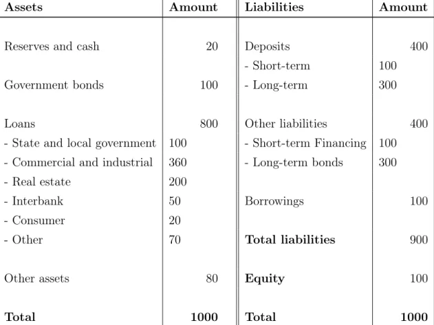
Under risk control we group the policies aiming to control the risks taken by financial institutions in their daily business. These policies generally impose some restrictions or requirements on the balance sheet of financial institutions (balance sheet regulation). The main idea here is to ensure an equilibrium between the risk taken by financial institution and their capital (or risk absorbing capacity).
The balance sheet of a financial institution can be seen as a list of its sources of funds (liabilities) and uses to which these funds are put (assets)2. It rep-resents, at a given time, an overview of the assets, liabilities, and equity a financial institution posses. Table 1.1 shows the balance sheet of an hypothet-ical commercial bank. For a detailed description of the items of this balance sheet we refer the reader to Mishkin and Eakins [2012], Chap. 17.
Assets Amount Liabilities Amount
Reserves and cash 20 Deposits 400
- Short-term 100
Government bonds 100 - Long-term 300
Loans 800 Other liabilities 400
- State and local government 100 - Short-term Financing 100 - Commercial and industrial 360 - Long-term bonds 300
- Real estate 200
- Interbank 50 Borrowings 100
- Consumer 20
- Other 70 Total liabilities 900
Other assets 80 Equity 100
Total 1000 Total 1000
Table 1.1: Bank balance sheet
2Financial institutions (financial intermediaries) generate fund by borrowing and by
is-suing liabilities (e.g. bonds and deposits). The generated funds are then used to finance assets (e.g. loans)
Note that the equity of a bank is defined as the difference between its assets and liabilities:
Equity=Assets−liabilities.
The primary way to regulate the balance sheet of financial institutions is to impose conditions on its capital.
Remark 1. Note that the capital of a bank consist mainly but not only of its equity. Other liability instruments can also count as bank capital. We have in this context:
Capital≥Assets−Liabilities.
One example of such a requirement imposed on bank capital are capital adequacy ratios (CAR):
CAR:= C
A ≥α
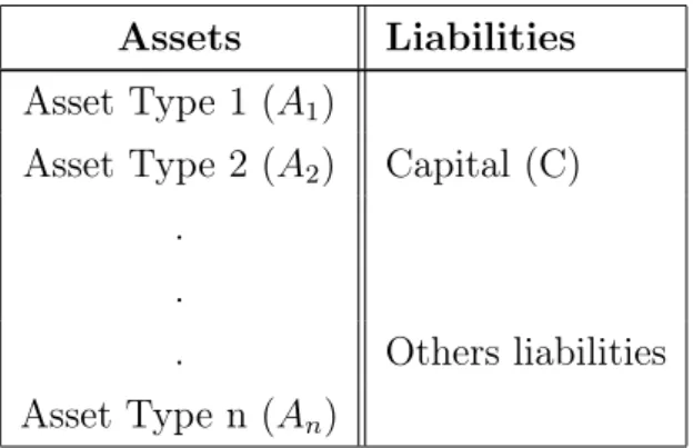
where C is the capital, A is the sum of all assets and α is a limit specified by the respective regulatory authority. In this context the balanced sheet of a bank can be reduced to the following representation:
Assets Liabilities Asset Type 1 (A1)
Asset Type 2 (A2) Capital (C) .
.
. Others liabilities Asset Type n (An)
Table 1.2: Reduced bank balance sheet
The CAR is often defined accordingly to the riskiness of asset types. This is done by assigning to each asset type (Ai) a risk weight (Wi).
CAR= n C
P
i=1
Ai×Wi .
This principle is followed by the Basel Committee on Banking Supervi-sion(BCBS). The BCBS was created by the Group of Ten (G-10) countries in the wake of the bankruptcy of the Herstatt Bank in 1974. Its mission is to contribute to the stabilization of the international financial system by defin-ing guidelines and recommendations of best practice for financial regulation
(the so-calledBasel Accords). The Basel Accords are not legally binding for single countries, but represent guidelines and recommendations that need to be translated into law.3 The first Basel Capital Accord is that of 1988 also known as Basel I. It is a risk-based capital regulation in the sense that it requires financial institutions to keep a minimum of capital, the so-called regulatory capital(RC), depending on the risk they take. This means that, the risks that a financial institution is allowed to take depends on its financial capital. Under Basel I the capital instruments are regrouped, depending on their capacity to absorb losses (quality) 4 into two categories: (i) Tier 1 capital (Core capital) and (ii) Tier 2 capital (supplementary capital). The total capital is defined as the sum of Tier 1 capital and Tier 2 capital.
• The Tier 1 capital consists of permanent shareholder’s equity and dis-closed reserves (retained earnings after tax).
• The Tier 2 capital consists of reserves, provisions, hybrid capital, subor-dinated debt with minimum maturity of 5 years.
Tier 1 capital are high-quality and consist primarily of equity. They are able to absorb losses in a going-concern basis, i.e on the assumption that the considered financial institution will still in business for an indefinite period whereas Tier 2 capital is supposed to absorb losses in a gone-concern, i.e. basis when the bank becomes insolvent.
Remark 2. A going-concern financial institution has positive equity capital.
In the context of the Basel accords the assets of financial institution are splitted into banking book, trading book and cash. The banking book contains assets that are assume to be held until the maturity (e.g. as loans). The trading book contains assets and instruments that are intentionally held for short-term resale or forhedging other instruments of the trading book.
Remark 3. These trading book assets are typically valuated on a mark-to-market basis using only quoted market prices. while banking books could be valuated at their original cost.
The Basel I focus credit riskarising from both, trading book and banking book. It required the ratio betweencapital of a bank and a weighted sum of
3For example, the Basel III is implemented in EU through Capital Requirements Directive
IV (CRD IV).
4Equity is for the Basel Committee the preferred eligible capital because it is permanent
all its assets (RW A) to be equal or greater than 8% (see Basel Capital Accord [1988]). The corresponding CAR is then:
CAR= Tier 1 capital + Tier 2 capital
RW A= n P i=1 RW Ai ≥0.08 with RW Ai =Ei×RWi,
wherenis the number of a bank’s assets includingon-balance sheetand off-balance sheet items excluding derivative items, Ei is the financial exposure
associated with asset i and RWi is the risk-weight associated with asset i.
Remark 4. Off-balance-sheet items doe not appear on the (current) balance sheet of financial institution. However, they could generate a loss in the future, hence affecting the future shape of balance sheet. Example of off-balance-sheet items are options and guarantees.
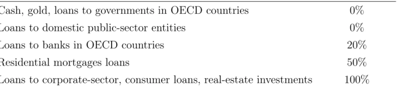
The assignment method of RW is defined by the BCBS in such a way to reflect the inherent risk (i.e. the probability of default and the expected loss in the case of a default) of the associated asset. In Basel I, they took only 5 values 0%, 10%, 20%, 50% and 100%. Table 1.3 shows a sample of risk weights for certain on-balance-sheet items as specified in Basel I. As we can see, cash and securities issued by governments of OECD5 countries are considered to be risk free and have then a risk weight of zero. Loans to corporations have a risk weight of 100%. Loans to banks and government agencies in OECD countries have a risk weight of 20%. Residential mortgages have a risk weight of 50%.
Asset Type Risk Weight
Cash, gold, loans to governments in OECD countries 0%
Loans to domestic public-sector entities 0%
Loans to banks in OECD countries 20%
Residential mortgages loans 50%
Loans to corporate-sector, consumer loans, real-estate investments 100% Table 1.3: Risk weights for certain on-balance-sheet items.
Remark 5. According to table 1.3, a bank that, has only exposures to OECD sovereign debt does not have to hold any regulatory capital (RC = 0), since the RW associated to loans to governments in OECD countries is zero.
5The group of countries that are full members of the Organisation for Economic
The RWA of off-balance sheet instruments is generally calculated in two steps
1. the nominal amountE of an off-balance sheet instrument is transformed into an equivalent on-balance sheet loan (credit equivalent amount). This is done by multiplying the principal amount of off-balance sheet instru-ment by a predefined credit conversion factor(CCF).
2. the appropriate risk-weight is assigned to the resulting equivalent credit.
The RW Ai off an off-balance instrument i is thus computed by
RW Ai :=Ei×CCFi×RWi.
Remark 6. In practice, the financial exposure Ei associated with an asset i
is estimated by the exposure at default (EAD). The formula for computing the RWA becomes,
RW Ai =EADi×RWi.
Basel I also requires at least 50% of the required RC to be in Tier 1. This means that the Tier 1 capital ratio, which is given by
Tier 1 capital ratio := Tier 1 capital
RWA ,
must be at least4% (Tier 1 capital ratio ≥0.04). For a more detailed under-standing of the weighting system and the capital definition in Basel I, we refer to Basel Capital Accord [1996]. The Basel accord evolved considerably since 1988. Changes in the Basel accord usually appear in the form of amendments or releases. These changes in the Basel accords aim to adapt the regulation framework to changes in financial markets or to react to a financial crisis. For example, a partial amendment of the accord of 1988 was made in 1996 (see Basel Capital Accord [1996]). It required banks to additionally allocate capital to cover market risk, i.e. risk due to movements in market values, such as interest rate risk, equity position risk, foreign exchange risk and commodities risk. It also defined a new category of eligible capital, that was exclusively eligible to cover market risk only. This capital is calledTier 3 capital.6
The corresponding CAR was then given by
CAR = Bank’s capital
Credit risk RWA + Market risk RWA ≥0.08
Remark 7. In practice the risk capital for credit risk (CRC: credit risk charge) and that of market risk (MRC: market risk charge) are computed separately. And the total risk charge (TRC) is computed as the sum of CRC and MRC.
The release of the Basel accord of 26 June 2004 (see Basel Capital Accord [2004]) also known as Basel II adopts the same philosophy as that of Basel I. It continues to apply a risk weights based CAR. However, it focuses not only on market and credit risk, but also considers operational risk, which is defined as the risk resulting from inadequate or failed workflow processes. It also changed the way as risk weights were calculated.
Note that one of the main problems in the Basel I accords is that the assign-ment method for the risk weights does not take into account the credibility of the borrower. For example, under Basel I, a bank that lent a given amount to a company with a good credit standing were obliged to hold exactly the same amount of regulatory capital as that he would if lent the same amount to a company on the edge of bankruptcy. Basel II has elaborated alternative meth-ods in which the credibility of the borrower is taken into account (or modeled) by its default probability (PD).
Basel II provided three different approaches for the determination of risk weights for credit risk: 1) the standardized approach (SA), 2) the foundation internal rating based approach (F-IRB) and 3) the advanced IRB approach. In the standardized approach (SA), the default probability of borrower depend on ratings provided by external specialized financial institutions, the so called credit rating agencies. In the IRB approach the default probabilities of borrowers are based on a bank’s internal rating system.7 Figure 1.1 illustrates the link between rating and risk weights for exposures to countries, banks, and corporations under Basel II’s standardized approach.
Figure 1.1: Rating vs. Risk Weights (in %). Source: Hull [2012]
Another innovation in Basel II is the adoption of a three "Pillar"-structure in the formulation of regulatory policies. Through this structure, the Basel
7This need to be approved by relevant regulatory institutions such as the BaFin
Committee aims at integrating the three main aspects of financial risk man-agement, namely the quantitative, qualitative, and market discipline (trans-parency) aspect in the regulation of the financial system.
1. Pillar 1 (quantitative aspect) provides the rule for the calculation of regulatory capital. It consists of similar risk capital ratios as Basel I and additionally considers operational risks.
2. Pillar 2 (qualitative aspect) provides principles for the supervisory review process. Following these principles a bank can estimate, using it own models, the capital that it needs to cover the economic effects of risk-taking activities and to secure the survival of its business on a going concern basis. This capital is called economic capital.
3. Pillar 3 (market discipline aspect) aims at promoting discipline and trans-parency in the financial system by calling on banks to disclose more information about the way they allocate capital and the risks they take.
Remark 8. Under Basel II, the capital requirements for the banking book was generally higher than that for trading the book. Some financial institutions used this gap and developed practice to reduce their regulatory capitals while holding the same risks (regulatory arbitrage). They transfer for this purpose their banking book assets to the trading book. This is done by first transform via secularization techniques the considered asset (e.g. a loan) into a tradable asset (e.g. a bond) then distributes them to other financial institutions.
As a reaction to the latest financial crisis the BCBS published in December 2010 a revision of the Basel accords, the so- called Basel III. As we can read in Basel Committee on Banking Supervision [2009],
”the objective of Basel III is to improve the banking sector’s ability to absorb shocks arising from financial and economic stress, whatever the source, thus reducing the risk of spillover from the financial sector to the real economy”.
This statement clearly asserts that the main focus of Basel III is the man-agement of systemic risk. The main aspects of Basel III are:
• The redefinition of the concept of eligible capital8. Under Basel III, the Tier 3 capital is eliminated and the Tier 1 capital is splitted into Com-mon Equity Tier 1(CET1) and Additional Tier 1 capital and the relative amount of tier 1 is increasing from 4% to 6%. This increases the
quality of regulatory capital. The augmentation of the regulatory capi-tal is assured by the introduction of three new capicapi-tal components such as the Capital Conservation Buffer, theCounter-Cyclical Buffer and thesystemic risk capital buffer for globally systemically im-portant banks (G-SIBs). The total risk capital is then:
TRC = Tier 2 + Tier 1+capital conservation buffer +countercyclical capital buffer
+systemic risk capital buffer for G-SIBs
• The difference in the treatment of systemically important institu-tions. These are for example required to hold extra regulatory capital (systemic risk capital buffer).
• The introduction of liquidity requirements, namely the liquidity cov-erage ratio (LCR) and the net stable funding ratio (NSFR). The LCR aims to ensure that banks have enough amount of unencumbered High-Quality Liquid Assets (HQLA)9 to withstand a period of 30-days of liquidity disruptions while the NSFR aims to ensure that sufficient funding is available in order to cover a period of at least one year.
• The introduction of requirements on leverage. The Basel III leverage ratio(LR) is defined by:
Leverage Ratio= Tier 1 capital Exposure measure
The exposure measure can be seen here as the sum of all a bank’s expo-sures (or all assets).
Remark 9. Contrary to others capital ratios the denominator of the LR is not the RWA.
1.1.3
Crisis management
With crisis management we refer to procedures aimed at managing financial institutions, being in critical situation, in an orderly way in order to preserve financial stability. Their main objectives are:
• avoid contagion effects,
• protect client funds,
• ensuring that the financial system’s banking services remain uninter-rupted10.
The commonly used instruments or tools, for the management of financial institutions being in a critical financial situation are:
• credit,
• asset purchases,
• liquidity facilities,
• guarantees,
• and nationalizations.
The use of these instruments generate costs, which need to be financing. This can be done using taxpayer’s money or via special fund called resolution fund. One of the prominent examples of crisis management operation are the Troubled Asset Relief Program (TARP) in the US and the quantitative easing (QE) program of the European central bank. The TARP was been signed into law in October 2008. The TARP provided to the US treasury a fund of $ 700 billion to purchase subprime and other mortgage backed securities from financial institutions in difficulty in order to stabilize the US financial system.11 The aim of the QE is to increase the money supply in the European financial system by buying securities, such as corporate and government bonds, from financial institutions.
Remark 10. Note that in the case of TARP and the QE the financial assis-tance given to financial institutions in difficulty is supported using external funds (provided by the governments and other financial authorities). This procedure corresponds to a Bail-out.
The bail-out of private financial institutions by government are very un-popular, because they involve a massive use of taxpayer money to finance the losses caused by financial institutions.12.
10This imposes a continuity of the essential (or critical) financial and economic functions
of unsound or failing financial institutions.
11Updated information about the recipients, the amount disbursed, the amount
re-turned, the revenues of the TARP program can be seen in the following web-page: https://projects.propublica.org/bailout/list.
12Bail-out can be interpreted by the taxpayer as if they have the obligation to participate
However, it is important to note that the cost generated by the collapse of real economies are generally very high13. Hence, to avoid the collapse of their financial system and their real economies some governments were forced to bail-out certain financial institutions. In fact, some financial institutions are considered so important (large and highly interconnected with other financial institutions) that their failure could potentially bring down an entire regional (domestic or global) financial system, thereby causing a high social and eco-nomic cost for governments and society as a whole. These financial institutions are commonly called ’too big to fail’.
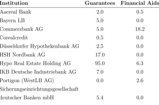
It is in this context that the German government has set up, in October 2008, a special fund called SoFFin (Sonderfonds Finanzmarktstabilisierung -Special Financial Market Stabilization Fund) for the financing of its bail-out actions. The SoFFin is administrated by the Financial Market Stabilisation Agency (FMSA) which was also in charge of the coordination of the bail-out actions taken by the German government.
Table 1.4: Bail-out recipients in Germany: Status: 31.12.2009, in bn EUR Institution Guarantees Financial Aids
Aaereal Bank 2.0 0.5 Bayern LB 5.0 0.0 Commerzbank AG 5.0 18.2 Corealcredit 0.5 0.0 Düsseldorfer Hypothekenbank AG 2.5 0.0 HSH Nordbank AG 17.0 0.0
Hypo Real Estate Holding AG 95.0 6.3 IKB Deutsche Industriebank AG 7.0 0.0
Portigon (WestLB AG) 0.0 2.6
Sicherungseinrichtungsgesellschaft
deutscher Banken mbH 5.4 0.0
The table 1.4 shows the actions and the recipients of the German bail-out operation per 31.12.2009.
The bail-out of financial institutions can be seen as an effective way to contain the propagation of financial distress across a financial system and the real economy. However, there are at least three aspects of the governmental bail-out actions that pose a problem:
13Example of the effect of crisis in the real economic are: reduction of consumption and
1. They are funded by taxpayer money.
2. The money used by the government for a bail-out action is generally transferred to other financial institutions and not to the real economic. As an illustrative example, the table 1.5 shows some financial charges assumed by the US government in the bail-out of the American Interna-tional Group (AIG).
Table 1.5: Collateral amounts posted by AIG to its counterparties after it began receiving government assistance. Data source: www.aig.com
Counterparty Amount Posted in Billion $ Country
Societe Generale 4.1 France
Deutsche Bank 2.6 Germany
Goldman Sachs 2.5 USA
Merrill Lynch 1.8 USA
Calyon 1.1 USA Barclays 0.9 UK UBS 0.8 Swiss DZ Bank 0.7 Germany Wachovia 0.7 USA Rabobank 0.5 Hollande KFW 0.5 Germany JPMorgan 0.4 USA
Banco Santander 0.3 Spain
Danske 0.2 Danmark
Reconstruction Finance Corp 0.2 USA
HSBC Bank 0.2 UK
Morgan Stanley 0.2 USA
Bank of America 0.2 USA
Bank of Montreal 0.2 Canada
Royal Bank of Scotland 0.2 UK
Other 4.1
Remark 11. Table 1.5 also highlights the internationalization of finan-cial transactions.
3. The bail-out of financial institutions by their respective governments implicitly implies that the stability of one given financial system (or financial sub-system) depends on the ability of the respective government
to bail-out (or to finance) the respective systemically important financial institutions.14 This poses a problem when the considered financial system encloses many governments such as theEurozone. Because the stability of such a financial system can only be assured if all its sub-financial system are stable, this requires a harmonized stability mechanism. The lack of harmonized stability mechanisms can lead to a political crisis. Recall that the Eurozone is a currency union with a common monetary policy under the responsibility of the European Central Bank (ECB) and with the Euro as common currency. One main aspect of the Eurozone is the liberalization of all legal financial transactions (capital flows and risk transfers) between financial institutions from different members coun-tries. This promotes the establishment of huge financial system called euro area.
The EU recognized these problems and reacted by elaborating harmonized frameworks for the management of failing financial institutions across the euro area. The main frameworks are:
• The Bank Recovery and Resolution Directive15(BRRD).16.
• The single Resolution Mechanism (SRM) and the Single Resolution Fund (SRF).
The BRRD provides a minimal17 harmonized legal framework for the man-agement of failing financial institutions without (or less) contagion effects18 and without resort to bail-out operations using public funds (resolution). It is builds on the following three main pillars (or tasks)
1. resolution planning: The scope of resolution planning is to develop res-olutions strategy and identify the obstacles to resolution operation that need to be addressed in order to facilitate the resolution operation if need be.
2. Mitigation of financial institution’s default. This is done using tools such as recovery operation (Sets of measures taken by a financial institutions
14From this perspective it is not a surprise why the financial crisis persists in Greece and
not in Germany
15see http://eur-lex.europa.eu/legal-content/EN/TXT/?uri=celex:32014L0059
16The BRRD is implemented in the German law through the Sanierungs- und
Abwick-lungsgesetz - SAG (see www.gesetze-im-internet.de/bundesrecht/sag/gesamt.pdf)
17The BRRD allows state to use their own recovery and resolution strategy, insofar as it
is not in conflict with the BRRD
in financial dificulty in order to restore its busness operations to a normal condition) and early intervention19.
3. resolution operation.
It provides to competent authorities legal instruments, which can be used for resolution purpose (resolution tools) . Examples of resolution tools are:
• the sale of business unit (Article 38 BRRD).
• the building of bridge institution(Article 40 BRRD). The is to transfer certain asset to a third-party financial institution.20
• separation of bank assets (Bad Bank, Article 42 BRRD). The aim of this instrument is to preserve the systematically relevant part of the failing financial institution whilst liquidating the non-systematically relevant part part.
• and bail-in (Article 43 BRRD). In fact, the BRRD stipulates that, should a bank fail, its shareholders, creditors and uninsured depositors should be first in line to assume losses if the bank gets into financial difficulty. This principle is called ’bail-in’.
In the context of BRRD, the bail-in is used as instrument to ensure the se-quential allocation of losses and the write down of the claims of shareholders, subordinated creditors, and senior creditors.
Remark 12. Depositors below EUR. 100,000 are in general excluded from suf-fering losses, their claims are protected by national Deposit Guarantee Schemes, such as the Einlagensicherungsgesetz21 in Germany or the Federal Deposit In-surance Corporation (FDIC) in the USA.
The BRRD is implemented in the euro area through the SRM. Under the SRM, resolution operations are funded by the SRF. The SRF is a resolution fund that is financed through the ex ante contributions of banks and cer-tain investment firms established in the countries subject to the SRM. The individual ex ante contribution is calculated, at least annually, by the SRB based on a method22, which takes into account the systemic importance of the focused financial institution and a predefined target level of 55 billion EUR
19see Articles 27-30 BRRD
20such as the Erste Abwicklungsanstalt (EAA) 21URL: http://www.gesetze-im-internet.de/einsig/
(1% of covered deposits of all credit institutions established in the countries subject to the SRM estimated on 2011 reported data).23 Following the BRRD requirements, the bail-in instrument has to be used before any public funds or SRF.
Remark 13. In case that the SRF is insufficient to finance a resolution oper-ation additional ex-post contributions could be collected.
The individual contributions are collected at a national level by relevant the relevant national resolution authorityNRA and transferred to thesingle resolution Board (SRB)24, which is an EU agency entrusted with the task to prepare resolution planning and to ensure the effectiveness of the resolution actions. To perform its tasks, the SRB uses two documents: 1) the recovery plan and 2)the resolution plan. The recovery plans are elaborated by the financial institutions, its show how they would act during financial turmoil in order restore their financial activities (financial continuity plan) and thus avoid liquidation and default. The resolution plans are elaborated by the resolutions authorities (the SRB and the NRA)25. It address how to handle a bank in resolution.26
Remark 14. Recovery plans are concerned by time before the default or resolution.
Remark 15. Generally bail-in operations (resolution operations in general) take place when the financial institution is still balance sheet solvent. The starting time and the magnitude of a bail-in operation is decided, based on some preamble analysis, such as the estimation of the potential financial loss suffered by the financial system if the considered financial institution fails and the impact of the planed bail-in operations on the corresponding financial sys-tem. For example, the
Article 44(3) of the BRRD gives resolution authorities the discretion to exclude or partially exclude certain bail-in-liabilities from the bail-in-operation (resolution), in exceptional circumstances, e.g. in the case that the assumed bail-in-operation could lead to a systemic risk.
23The data necessary for the calculation are reported to the SRB via the relevant national
resolution authority
24https://srb.europa.eu/
25Following Articles 10-14 of the BRRD resolution plans are elaborated by national
reso-lution authorities under the supervision of the SRB
26To facilitate their work, the resolution authorities can require financial institutions to
The capital generated by a bail-in operation may be insufficient to absorb a loss entirely. The effectivity of a bail-in operation depends thus on the loss absorbing capacity of the involvedBail-in liabilities(i.e. the set of liabilities that are eligible to be written down or converted into equity by a bail-in operation). That is the motivation behind the definition of two ratios:
• The minimum requirement of own funds and eligible liabili-ties(MREL) for all financial institutions in the European Union27
• and thetotal loss-absorbing capacity(TLAC) for all Global System-atically Important Banks.
The aim of these two measures is to require financial institutions to main-tain a minimum amount of liabilities (bail-inable liabilities) that should be sufficient to adsorb losses in case of a bail-operation.
There are in the financial market some securities that behave as eligible li-abilities, but whose management is not assumed by a resolution authority but by their respective contract terms. The most prominent example of such in-struments is thecontingent convertible bond(CoCo-bond). Traditionally, convertible bonds are usual corporate bonds where the investor has theright but not the obligation to convert the bond into shares.28 A CoCo-bond is different in that the conversion of the bond into equity or the write-down of the bond face value is triggerautomatically when a certain contractual pre-definedtrigger conditionsis satisfied.29 The trigger conditions are typically defined based on regulatory capital ratios such as the Common Equity Tier 1 (CET1) ratio. In this context CoCo-bonds can be see as a supplementary cap-ital that adjust (increase) the capcap-ital of financial institutions in difficulties30in order to allow them to meet the regulatory capital ratios. furthermore, under CRD IV CoCo-bonds are allowed to count as Additional Tier 1 this means that CoCo-bond can account up to 1.5% of a bank RWA.
Remark 16. Note that, for the CoCo-bonds, the conversion or the haircut takes place when the bank is still a going concern (i.e. has positive equity capital), while a bail-in operation takes place when the bank is almost collapsed.
27Article 45 BRRD
28Typically the investor chooses to convert the bond into share when the stock price is
high
29A CoCo-bond can have more than one trigger condition. In this case the conversion or
the write-down is triggered when at least one condition is satisfied
1.2
Motivation and Contribution
1.2.1
The need for Macro-Prudential Regulatory Policies
One of the main gaps in the pre crisis financial stability policies was that the problem of financial stability had been considered only from a micro per-spective (micro-prudential regulation). The regulatory authorities tried to ensure the stability of entire financial system by reducing the probability of default of individual financial institutions in isolation.
This was incorrect. The evolution and internationalization of financial mar-kets and financial services has contributed to the establishment of a globally interconnected andpartially non-regulated31financial system concentrated around a few big financial institutions. As an illustrative example, Fig-ure 1.2 shows how the primary-secondary market design for government debt is concentrated around a few financial institutions known as primary dealers32, that have the exclusive authorization (privileges) to act as initial buyer for securities issued by the government.
As observed in the last crisis, the links between financial institutions provide a channel through which individual risks or failures can spread across the financial system. This is the macro nature of financial risks (macro-financial risk) that was ignored and that the regulatory authorities need to face now in order to stabilize the modern financial system.
In this context, the stability of the financial system can only be assured by regulatory policies that also take into account the potential contagion risk resulting from the interactions of financial institutions within the financial system. Such regulatory policies should aim at meeting the following two objectives:
1. make the failure of individual financial institutions less likely
2. reduce the impact of the failure of a single financial institution on the financial system (reduce the contagion effect).
Direct consequences of the last financial crisis are the measures adopted by governments and regulatory institutions to address the problem of the man-agement of systemic risks. Some important measures are:
31Since OTC market was not regulated at this time.
32The main activity of a primary dealer is to buy government securities in the primary
market and to resell them in a secondary market (typically over-the-counter) to other finan-cial institutions
Figure 1.2: Schema of the primary-secondary market system. The government is in the middle and acts as the primary issuer of securities. The dealers are represented by the large boxes containing number. End-users are symbolized by smaller boxes containing letters. The bold arrows represent the primary market and the light arrows represent the secondary market.
1. The treatment of financial institution depending on their systemic im-portance. three categories of SIFIs are defined for this purpose: 1) global systemically important financial institutions (G-SIFI), that is a finan-cial institution whose failure could have a negative impact on theglobal financial system , 2) domestic systemically important financial institu-tions (D-SIFIs) and 3) non systemically important financial instituinstitu-tions (N-SIFIs). The systemic importance of a financial institution depends on the effect that its failure could have on a financial system. This can be estimated by analyzing its size, the nature of its activities and the contracts it has entered into with other financial institutions (i.e. its degree of inter-linkage with the rest of the financial system)33. Global systemically important banks (G-SIBS) are, due to their system rele-vance, subject to stricter regulatory rules than other banks. They are for example required to hold a certain amount of bail-in eligible liability (Total Loss Absorbency Capacity: TLAC). This measure aims to ensure an effective bail-in operation in case it is needed.
33The Basel Committee uses a scoring methodology to determine which banks are G-SIBs
2. The elaboration of resolution plan. Note that, following BRRD the res-olution plans of a given financial institution has to elaborated by the respective resolution authority based on an analysis of the effect of the failure of this institution on the financial system.
3. The requirement by some governments and financial authorities for fi-nancial institution to contribute to the funding of aResolution Funds, for example theFinancial Crisis Responsibility Feein the USA and the Single Resolution Fund in the countries subject to the SRM.
4. The requirement standard over-the-counter (OTC) derivatives contracts to be cleared through an eligible central counterparty (CCP)34. CCPs manage their financial risk by requiring their members to provide ade-quate amounts of collateral(in the form of variation and initial margin) and to make contributions to a so-called default fund (or guarantee fund). Default funds are used by CCPs to absorb losses that cannot be covered by the collateral posted by a defaulting CCP member. Doing this, the CCP distributes the losses of defaulting members among the non-defaulting members. For more details on the functions CPPs, we refer the reader to Loader [2002].
Remark 17. The use of CCPs contributes to the stabilization of the financial system by managing the financial system losses due to the de-fault of OTC market participants and by simplifying and increasing the transparency of the derivatives market transactions. However, they are, because of their size and function, systematically important.35
Remark 18. The points 3) and 4) are in some sense methods to mutualize losses from individual defaults. In this context, the risk associated to an indi-vidual financial institution should not only depend on its idiosyncratic risk but also on the idiosyncratic of other financial institutions in the same financial system as well as their interdependency (systemic risk contribution with the CCP as financial system).
An effective estimation of systemic risk contribution in general and in partic-ular an understanding of the way how factors such as the size and interdepen-dency of financial institutions in distress can influence the financial system, is preeminent for solving the problem posed by the implementation of the above measures. The main problem here are:
34By the European Market Infrastructure Regulation (EMIR)
• The identification of the systemically important financial institutions (in particular, G-SIBs, D-SIBs and N-SIBs)
• The estimation of individual contribution to a mutual default fund. This necessitates the definition and computation of new types of measures of financial risk that are able to estimate systemic risk contribution.
This problem poses a new challenge for academics and regulatory insti-tutions, since the common risk measures such as Value-at-Risk (VaR) and Expected Shortfall (ES) only focus on one institution in isolation, thus ignor-ing the interdependence between financial institution and the related possible contagion effect.
1.2.2
CoV aR
-Method as a Tool for the estimation of
Sys-temic Risk Contributions
TheCoV aR-method of Brunnermeier and Adrian [2011] is the most used tool for the analysis of systemic risk. It builds on the termCoV aR. This is defined as the Value-at-Risk (V aR) of a financial system conditional on a given state of the considered single financial institution.
Contrary to the traditional financial risk measures, e.g. V aR and ES36,
CoV aR not only involves variables characterizing the univariate behavior of the considered financial institution in isolation (e.g. its loss) but also variables characterizing the univariate behavior of the entire financial system as well as variables characterizing the joint behavior of the considered financial institu-tion and the financial system (e.g. the correlainstitu-tion coefficient between their losses). This allowsCoV aRto integrate the interdependency structure (or the link) between the considered financial institutions i and the financial system
s, thus enabling it to describe the systemic risk contribution among financial institutions.
However, the calculation methods proposed so far for the estimation of
CoV aR are restrictive. Brunnermeier and Adrian [2011] for example adopted a statistical approach (i.e. no closed form or analytical formula) which is based on normal linear quantile regression (cf. Koenker and Bassett [1978]), Jäger-Ambrożewicz [2010] developed a closed formula for the special case where the losses of the financial institution and that of the financial system in focus are modeled by a bivariate normal distribution.
36These financial risk measures only consider variables characterizing the financial
The estimation methods cited above have their relative advantages and dis-advantages but they share the common restriction that both impose a bivariate normal distribution as a stochastic model. It is well known that the bivari-ate normal distribution can lead to difficulties relative to the modeling of the single marginal variables of a multi-variate stochastic variables as well as the respective joint stochastic behavior (or dependence structure).
In fact, the bivariate normal distribution imposes the univariate normal distribution as a model for univariate margins and the linear correlation coef-ficient as the unique dependence parameter. Based on the fact that the linear correlation coefficient measures only linear dependence and is controlled by movements around the mean of the distribution while movements in the extreme are neglected and considered as abnormal, we think that the linear correlation coefficient is not the appropriate measure of dependence for the analysis of systemic risk contribution.
Note that, in general, institution defaults and systemic crisis can be consid-ered as extreme events. Indeed, the default that produces the contagion effect corresponds generally to a shock (large loss) relative to an expected loss. This can be characterized by an extreme value which appears in the tails of the corresponding loss distributions.
Hence, systemic risk contribution is particularly concerned with the proba-bility of simultaneous large losses and hence with the tail of the loss distri-butions. Therefore, the analysis of systemic risk should be based on models which are able to specify how extreme losses are interdependent.
In this thesis we propose formulas for computing CoV aR in a general stochastic setting. Doing this we provide a flexible framework for an effec-tive analysis of systemic risk contribution. In chapter 4.1, a general formula for the computation of CoV aR in a wide stochastic setting is provided. This formula is derived using the theory of bivariate Copula functions, which is introduced beforehand in chapter 3.
Bivariate copula functions represent a class of bivariate distribution func-tions defined on the unit square [0,1]2 with uniformly standard distributed margins. The power of copulas is their ability to describe the dependence struc-ture of bivariate random vectors separately of their marginal distributions. In particular the theorem of Sklar [1959] allows to decompose any multidimen-sional joint distribution function into its univariate marginal distributions and a copula which models the entire joint behavior on a quantile scale. These features give the copula the ability to represent joint distribution with univari-ate margins of different types and to describe dependence structure precisely
in any region of joint distribution. It is for this reason that we use copula in order to model precisely extreme co-movement and hence contagion effects. By connecting theCoV aRconcept to copula’s theory we develop an analytical formula allowing the analysis and the computation ofCoV aR for a more gen-eral stochastic setting than only the normal distribution setting. We apply our formula to the Gaussian and the non-Gaussian setting. As non-Gaussian set-ting we consider the class of elliptical and Archimedean copulas as well as the convex combination of copulas. In chapter 6, we consider the CoV aR under elliptical distribution. The assumption of elliptical distributions, as model for the computation of CoV aR, represents a good compromise between the need of pragmatical and practicable risk measure for the definition of regulatory rules on the one hand and the need of flexible and consistent risk measure for the analysis of systemic risk contribution on the other hand.
Both approaches allow to consider not only the normal dependence models, especially those which are appropriate for the modeling of the simultaneous (tail) behavior i.e. model with positive tail dependence coefficient.
One another main contribution of this thesis is the critical analysis of the
CoV aR-method. By providing an example in which the CoV aR-method do not takes into account of the effect tail dependence, we show that theCoV aR -method as provided by Brunnermeier and Adrian [2011] is in general not sensi-ble to tail effect. Also, we highlight the fact theCoV aR-method is not coherent with the phenomena of contagion effect. We propose alternative models that cover these gaps.
Modeling Systemic Risk
Contribution
An effective modeling of systemic risk contribution requires an understanding of how the modern financial system works, how individual financial institutions and different financial risks are related and how their interaction can lead to systemic crises. For more details about this topic we refer to Claessens and Forbes [2014]. In this chapter, we will give, from a quantitative risk management perspective, a basic understanding of the notion of systemic risk contribution. Then, based on this, we will introduce theCoV aR-method as a model for the analysis of systemic risk contribution.
2.1
Financial System and Systemic Risk
The quantitative analysis and modeling of systemic contribution requires an understanding of the notion of a financial systems. It is thus important to precise some important notions that are related to financial system and systemic risk.
A financial system can be seen as a network of institutions in which funds and financial services are moving across time and space from one institution to an another institution (e.g. from a bank to a firms). For a detailed analysis of the notions of a financial system, we refer the reader to Schinasi [2005], Neave [2010] and Mishkin and Eakins [2012].
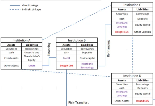
One of the main aspect of the modern financial system is the existence of a huge number of direct-1 and indirect-2 contractual linkages between financial
1e.g. between buyer and seller of CDS
2e.g. when many financial institutions undertake correlated or common risky investments
exposing therefor themselves to common risk factors 23
institutions. This is illustrated in figure 2.1. Hence, financial institutions, that consist a financial system, have exposures to each other. So, in case of the default of one financial institution the other financial institutions could be negatively affected. This provides a channels through which individual failures can spread across the financial system and thus undermine financial stability.
Figure 2.1: Financial linkages
The term systemic risk refers in general to the risk of collapse of an entire complex system as a result of the actions taken by the individual components that comprise this system. Systemic risk in financial systems can be defined as the risk that an initial default by one financial institution threatens the stability of the whole financial system by causing, via different propagation mechanisms, the default of other financial institutions of the system. This description corresponds to the view of systemic risk in a narrow sense (cf. De Bandt and Hartmann [2000] and De Bandt, Olivier and Hartmann, Philipp and Peydró, José Luis [2012]). Systemic risk in thebroad sense is caused by acommon shockto many financial institutions or an entire financial system. In this thesis i assume the systemic risk in a narrow sense .
The initial default that give rises to systemic risk is calledsystemic event (from a narrow sense perspective). Such a systemic event was the failure of Lehman Brothers on 15th. september 2008, which is assumed to be the
systemic event of the recent financial crisis.
Assumption 1. We consider here the systemic risk in the narrow sense. That is, we assume that systemic risk is caused by an initial default by one financial institution, that then spread in the whole financial system.
The mechanisms by which the failure of a financial institution spreads in the whole financial system is referred to contagion effect(cf. e.g. Allen and Gale [2008] or Allen and Gale [1998]).
Contractual or economical linkages between financial institutions are an im-portant transmission channels of contagion but not the only one. In fact, they are two main classes of contagion channels. The first is the fundamental channel. It the part of shock transition that could be completely explained using economic elements such as changes in ECB interest rates or the price of energy. The second is so calledinformational channel. It is the part of shock transition that can not be explained using fundamental economic analysis. It can be seen as the result of actions taken by economic participants or agents (such as fund manager or broker) based on a subjective (emotional) interpre-tation of financial news. For example, if one systemically important financial institutions defaults, the market will generally expected a negative trend in the whole financial system. This could have the following consequences.
1. A reduction in depositors confidence. As a consequence several severs could close out their accounts causing thus a liquidity crunch for the financial institution.
2. Thedecreasing in ratings of financial institutions. As a consequence, the funding cost of financial institutions will increase. This might leads to a situation in which the financial institutions are not able to satisfy their financial obligations and hence become distressed.
Remark 19. It is important to note that informational contagions leads in general to a liquidity risk and market risk, while fundamental contagions lead in general to a (counterparty) credit risk.
2.2
Basic Stochastic Model for Systemic Risk
The existing quantitative methods for the analysis of systemic risk can be summarized into two main approaches.
The first approach compares the linkages between financial institutions (or markets) during a relatively stable period with the linkages during an un-stable period. This approach is supported by many empirical studies. For example, Dobric et al. [2007] show that there are differences in the dependence structures of stock returns in bull and bear markets. There are also many studies that assert that the dependence between financial returns increases as the market is going down.
The second approach consists to model the direct linkage between financial institutions using network theory. The direct contagion mechanisms are then analyzed via simulations or stress-tests (cf. e.g. Cont et al. [2013] or Reyes and Minoiu [2011]).
The models considered in this thesis follow the first approach. We denote by i the financial institution in focus and by s the corresponding financial system. The loss taken by i and s are modeled following McNeil et al. [2005] (Section 2.1) respectively by the positive random variables Li and Ls, which
are defined on a probability space (Ω,F, P r). The distribution functions of
Li and Ls are denoted by Fi and Fs respectively. The interconnectedness of the financial institutioni to the financial systems is modeled by the degree of dependence between Fi and Fs. This is done by assuming that the random
variablesLi and Ls are stochastically dependent and that their joint behavior
is described by a bivariate joint distribution function.
Assumption 2. We consider only random variables which have strictly pos-itive density function. So, if a bivariate joint distribution function is consid-ered, it is assumed that it has a strictly positive density and that its marginal distributions have strictly positive densities.
Due to this assumption all distribution functions considered in this thesis are assumed to be absolutely continuous and strictly increasing.
2.3
Systemic Crisis and Financial Extreme Events
Systemic crises are closely related to two kinds of extreme events. First, the default of one systemically relevant financial institution (financial default) and second, the propagation of failures across financial institutions after the failure of one system relevant financial institution (contagion effect).
2.3.1
Financial Default and Extremes Events
From a quantitative risk management view, the failure of one financial insti-tution is the consequence of the realization of a large loss. Intuitively, such an event can be interpreted as an extreme value appearing in the upper tail region of the corresponding loss distribution. Mathematically, the notion of a financial distress can be characterized using special function called financial risk measure.
Definition 1. Let L be the class of losses defined on a probability space (Ω,F, P r). A mapping R:L →R is called a monetary measure of risk if it satisfies the following conditions for all L1, L2 ∈ L
1. Monotonicity: If L1 ≤L2 a.s., then R(L1)≤ R(L2)
2. Cash invariance: If L∈ L and l ∈R then R(L+l) = R(L) +l
Then, from the cash invariance property is motivated by the interpretation of R(L) as regulatory capital. It suggests that the financial risk measure associated to a lossLcan be adjusted by an amountlby adding or subtracting a deterministic quantity l toL.
A loss L such that R(L) ≤ 0 is called acceptable in the sense that a financial institution whit loss L is not required by the regulator to keep any regulatory capital. The set of acceptable losses associated with a risk measure
R is given by
AR={L∈ L | R(L)≤0}.
That is, a lossL isacceptablewith respect to the risk measure Rif L∈ AR. Let L be a non-acceptable loss i.e. L /∈ AR. By adding to L a positive cash amount of R(L), we define an adjusted loss (cf. McNeil et al. [2005], Section 6.1)
˜
L:=L− R(L).
Then, from the cash invariance property of monetary risk measures we have
R( ˜L) =R(L− R(L)) =R(L)− R(L) = 0,
so that L˜ ∈ AR. Hence, one can interpret R(L) as the minimum amount of capital that a financial institution with a loss L should keep as regulatory capital. In this context the monotonicity property implies that financial insti-tutions with higher losses need higher risk capitals.
Recall that, from a purely economic point of view, financial distress may be defined as a situation where a financial institution’s operating cash flow are not sufficient to satisfy current obligations (cf. e.g. Ross et al. [1999], A7 3.1). From a quantitative risk management perspective, given a monetary measure of riskRC, we can define distressed financial institutions as follows.
Definition 2(Distressed financial Institutions). LetL be the loss of the finan-cial institutionB. Let RC be the regulatory capital associated with the loss L. Let l be the realization ofL at the timet. We say that the financial institution
B is in distress at the time t iflis greater than the associated regulatory capital
RC, i.e.
l > RC.
If we assume that the regulatory capital RC is determined by a risk measure such as the Value-at-Risk (i.e. we assume that RC:=Value-at-Risk), then we say that the financial institutionB is in distress at time t if
l >Value-at-Risk. (2.1)
2.3.2
Contagion Effect and Extreme dependence
Contagion effect and systemic risk are closely related to the mathematical concept of extreme dependency.
Remark 20. During the crisis, (many) asset prices, independent of their re-spective nature, tend to move in the same direction. this increases the probabil-ity that single financial institutions fail together with the whole financial system or that a large number of financial institutions fail simultaneously. This phe-nomenon is well captured by the figure 2.2. It shows three periods of financial crisis (1930-1940, 1980-1994 and 2008-2014). Each period is characterizing by a concentration of massive simultaneous financial institution defaults.
In fact, as observed by many authors e.g. Chan-Lau, Jorge A. ; Mathieson, Donald J. ; Yao, James Y. [2002], the dependence between asset returns are often higher during the crisis than in normal situation. This can be explained by the fact that in normal situation the dependencies between assets prices are a reflection of their fundamental properties (for example similar assets tend to move in similar ways). But, this situation changes in a crisis or more pre-cisely after a shock. The behavior of the assets prices is in this situation much more affected by the measures taken by the financial market participants as
Figure 2.2: Bank Failures in the United States, from 1934 to 2015. (Source: Federal Deposit Insurance Corporation (FDIC)
reaction to the shock. These can be based on fundamental or informational point of view. A typical example, that describes how the actions taken by financial market participants can change the dependence between asset prices, is described in Brunnermeier and Pedersen [2009]. The authors showed how firesale3 can create new forms of dependence between assets held by similar in-vestors by adversely impacting on the asset prices of other financial institutions (see figure 2.3).
In this context, an increased in the dependency can be see as feature of fi-nancial market turmoil and fifi-nancial crisis. Following this, Forbes and Rigobon [1999] defined contagion as a significant increase in financial market linkages af-ter a shock to one market (or a group of markets). This definition means that, contagion effects are the consequence of a significant increase in the interde-pendence of financial institutions after a systemic event. In the same sense , Brunnermeier and Adrian [2011] argue that "the main idea of systemic risk measurement is to capture the potential for the spreading of financial distress across institutions by gauging the increase in tail co-movement".
From a probabilistic point of view, a contagion effect may be seen as a phe-nomenon in which the failure of one financial institution increases the proba-bility of the failure of other financial institutions. This can be characterized by a raise of the probability of simultaneous large losses. Therefore, in the analysis of contagion effects and hence of systemic risk contributions we are particularly interested in the dependence structure in the upper tails of joint
3This can happen because the considered financial institutions suffers from a lack of
Figure 2.3: Loss spiral: Source Brunnermeier and Pedersen [2009].
loss distributions. Notice that, if losses are independent in the tail of the joint loss distribution, large losses and hence the failures of financial institutions appear to occur independently of each other. Hence, there would be no conta-gion effect and the systemic risk contribution of the respective element of the system would be equal to zero.
It is thus important to model the extreme (or tail) dependence when an-alyzing systemic risk contribution. In the next section, we present the usual approaches for the modeling of tail dependence.
2.3.3
Measuring the Dependencies of Extreme Events in
Finance
There are two different approaches for modeling extreme dependence. The first approach consist to describe extreme dependence by considering a "con-ditional" or "local"-version of an existing dependence measure. The second consist to describe the dependence in the tail region of the assumed distribu-tion using condidistribu-tional probability.
Conditional Correlations Coefficient
The Conditional Correlations Coefficient is the typical example of the first approach. The idea behind conditional correlation is to measure the
correla-tion between financial institucorrela-tions condicorrela-tioned on certain extreme events, for example extreme losses (co-exceedance correlation).
Definition 3(cf. Malevergne and Sornette [2006], Definition 6.2.1). LetX and
Y be two real random variables andC a subset ofRsuch thatP r(Y ∈C)>0. The conditional correlation coefficient ρC of X and Y conditioned on Y ∈ C
by definition, can be expressed as
ρC =
Cov(X, Y|Y ∈C)
p
V ar(X|Y ∈C)·V ar(Y|Y ∈C). (2.2) So, by defining C := [v,+∞), it is possible to examine whether a model is asymptotically dependent by making v tend to ∞. For example, in the case that the variables X and Y have a bivariate normal distribution with an (unconditional) correlation coefficient ρ, we have the following theorem. Theorem 1 (Boyer et al. [1999], Theorem 1). Consider a pair of bivariate normal random variables X andY with variances σ2X and σ2Y respectively, and covariance σXY. Set ρ = σσXY2
Xσ
2
Y
, the unconditional correlation between X and
Y. Consider any event Y ∈ C, where C ∈R such that 0 < P r(Y ∈C) <1. The conditional correlation ρC between X and Y, conditional on the event Y ∈C, is equal to ρC := ρ q ρ2+ (1−ρ2) V ar(X) V ar(X|Y∈C) . (2.3)
Malevergne and Sornette [2006] show that for large v the formula (2.3) may be transformed into the following closed formula (cf. Malevergne and Sornette [2006], Formula (6.3)): ρC ∼ lim v→∞ ρ p (1−ρ2) 1 |v|. (2.4)
This slowly goes to zero as v goes to infinity. That is, the bivariate normal distribution is asymptotically independent and is therefore not a good model for the analysis of systemic risk contributions. A detailed theoretical back-ground about conditional correlation in particular and conditional dependence in general could be found in Malevergne and Sornette [2006] Chapter 6.
Tail dependence coefficient
The main idea of the measurement of extreme dependence via the coefficient of tail dependence4, is to describe the dependence in the tail region of the dis-tribution through a conditional probability. LetX and Y be random variables
4For more details about the measures of dependence between a pair of random variable
with the joint distribution function H and univariate marginal distribution functions F and G, respectively. If P r(X > x) > 0, then the dependence in the upper tail region of the distribution may be expressed by
P r(Y > y|X > x) = P r(X > x, Y > y)
P r(X > x) . (2.5)
By replacing in equation (2.5)xandyby theirα-quantilesF−1(α)andG−1(α) respectively, we obtain the tail dependence measure χ(α) (cf. Coles et al. [1999]).
χ(α) =P r Y > G−1(α)|X > F−1(α)
(2.6)
χ(α) measures the probability that Y exceeds G−1(α) given that X ex-ceedsF−1(α). In the context of the analysis of systemic risk contribution the equation (2.6) can be used to express the probability that the financial sys-tem s undergoes a large loss given that the single financial institution i also undergoes a large loss. From this perspective the tail dependence measure
χ(α) = P r Ls> Fs−1(α)|Li > Fi−1(α)
(2.7)
can be seen as a natural indicator of the potential contagion effect (and hence systemic risk contribution) from financial institutionion the financial system
s over a given threshold α.5
χ(α) expresses for α → 1 the probability of extreme co-movements and corresponds to the well-known upper tail dependence coefficientλu.
Definition 4(cf. McNeil et al. [2005] Definition 5.30). Let(X, Y)be a bivari-ate random variable with marginal distribution functionsF andG, respectively. The upper tail dependence coefficient of X and Y is the limit (if it exists) of the conditional probability that Y is greater than the 100α−th percentile of G
given that X is greater than the 100α−th percentile of F as α approaches 1, i.e.
λu := lim
α→1−P r Y > G
−1(α)|X > F−1(α)
. (2.8)
If λu ∈ (0, 1] then (X, Y) is said to show upper tail dependence or extremal
dependence in the upper tail; ifλu = 0, they are asymptotically independent in
the upper tail.
Similarly, the lower tail dependence coefficient λl is the limit (if it exists) of
the conditional probability that Y is less than or equal to the 100αth percentile
![Figure 1.1: Rating vs. Risk Weights (in %). Source: Hull [2012]](https://thumb-us.123doks.com/thumbv2/123dok_us/9006030.2798376/14.892.187.749.869.979/figure-rating-vs-risk-weights-source-hull.webp)


![Figure 2.3: Loss spiral: Source Brunnermeier and Pedersen [2009].](https://thumb-us.123doks.com/thumbv2/123dok_us/9006030.2798376/37.892.150.678.138.476/figure-loss-spiral-source-brunnermeier-and-pedersen.webp)
