doi:10.1017/S0022112009992965
Large-eddy simulation of mixing in a
recirculating shear flow
G E O R G I O S M A T H E O U,1†A R I S T I D E S M. B O N A N O S,1 C A R L O S P A N T A N O2 A N D P A U L E. D I M O T A K I S1
1Graduate Aeronautical Laboratories, California Institute of Technology, Pasadena, CA 91125, USA
2Department of Mechanical Science and Engineering, University of Illinois at Urbana-Champaign, Urbana, IL 61801, USA
(Received23 April 2009; revised 22 October 2009; accepted 22 October 2009)
The flow field and mixing in an expansion-ramp geometry is studied using large-eddy simulation (LES) with subgrid scale (SGS) modelling. The expansion-ramp geometry was developed to investigate enhanced mixing and flameholding characteristics while maintaining low total-pressure losses. Passive mixing was considered without taking into account the effects of chemical reactions and heat release, an approximation that is adequate for experiments conducted in parallel. The primary objective of the current work is to validate the LES–SGS closure in the case of passive turbulent mixing in a complex configuration and, if successful, to rely on numerical simulation results for flow details unavailable via experiment. Total (resolved-scale plus subgrid contribution) probability density functions (p.d.f.s) of the mixture fraction are estimated using a presumed beta-distribution model for the subgrid field. Flow and mixing statistics are in good agreement with the experimental measurements, indicating that the mixing on a molecular scale is correctly predicted by the LES– SGS model. Finally, statistics are shown to be resolution-independent by computing the flow for three resolutions, at twice and four times the resolution of the coarsest simulation.
1. Introduction
Mixing on a molecular scale of two or more fluids of different composition is achieved by the action of diffusion. The rate of mixing of different species is of primary importance in combustion applications because the speed of chemical reactions is determined by the availability of mixed reactants and the rate of chemical reaction once the reactants are mixed. For fast kinetics, chemical-product formation is limited by the molecular mixing rate. Specifically, combustion in non-premixed systems, the category of flows of interest in this work, can only occur when a mixture of fuel and oxidizer is homogenized on a molecular scale. Hence, in the present discussion, the term mixing will refer to molecular mixing of scalar quantities, such as species mass fractions.
In studies of turbulent mixing, jets and shear or mixing layers (Brown & Roshko 1974; Konrad 1976; Mungal & Dimotakis 1984; Papamoschou & Roshko 1988; Hermanson & Dimotakis 1989) are two canonical flows that have been used most
widely. Entrainment and growth rate processes in incompressible shear layers are well understood (Dimotakis 1986, 1991), despite the fact that prediction of the growth rate appears to be sensitive to the inflow conditions (e.g. George 1989; Slessor, Bond & Dimotakis 1998), with important implications for the simulation of such flows. For incompressible gas-phase shear layers, about half the fluid within the layer is mixed on a molecular scale (Dimotakis 1991).
Mixing in compressible shear layers has not been as well characterized. The growth rate of the mixing zone, which sets an upper bound on mixing, decreases with increasing compressibility (Papamoschou & Roshko 1988; Slessor, Zhuang & Dimotakis 2000). However, contradictory trends are reported for the dependence of the fraction of the mixed fluid in the mixing layer on compressibility (Hall, Dimotakis & Roseman 1991; Island, Urban & Mungal 1996; Freund, Lele & Moin 2000; Rossmann, Mungal & Hanson 2004).
Turbulent jets represent another canonical flow that has been studied. The jet in crossflow (Pratte & Baines 1967; Andreopoulos & Rodi 1984; Andreopoulos 1985; Smith & Mungal 1998; Shan & Dimotakis 2006) is characterized by higher entrainment rate than a jet into a quiescent reservoir (e.g. Becker, Hottel & Williams 1967; Dowling & Dimotakis 1990; Miller & Dimotakis 1996). In supersonic crossflow (Zukoski & Spaid 1964; Spaid & Zukoski 1968; Hollo, McDaniel & Hartfield 1994; Ben-Yakar, Mungal & Hanson 2006), a bow shock forms, causing the boundary layer to separate, creating a flameholding region where fuel and air can mix subsonically. However, this comes at a penalty of high total-pressure losses.
Predictive simulation of turbulent mixing is a valuable tool for understanding the process of entrainment and the subsequent homogenization of the mixture, especially in complex flow configurations. In most flows of practical interest, the Reynolds number is high, well above the mixing-transition Reynolds number (Dimotakis 2000), resulting in a broad range of spatial and temporal flow scales that place direct numerical simulation (DNS) beyond practical reach.
Large-eddy simulation (LES) is a method developed to capture the behaviour of turbulent flows. In LES, large-scale turbulent motions are resolved, whereas scales below a certain cutoff are modelled. The smallest scales contain only a small fraction of the turbulent kinetic energy, are more homogeneous and (hopefully) universal and expected to be less sensitive to modelling assumptions (e.g. Tennekes & Lumley 1972; Pullin 2000; Pope 2004b).
LES has been successful in the simulation of many non-reacting flows (Lesieur & Metais 1996; Piomelli 1999; Meneveau & Katz 2000) but the simulation of turbulent mixing in reacting and non-reacting flows still presents many challenges (Pitsch 2006). Turbulence models for momentum transport rely on theoretical constructs like the eddy cascade and scale invariance in the inertial subrange. On the other hand, mixing on a molecular scale takes place only at the smallest scales of the flow (Dimotakis 1991, 2005; Warhaft 2000) and cannot be resolved by the computational grid. Therefore, LES models must ‘infer’ subgrid mixing based on the resolved scales. Turbulent mixing in reacting flows presents additional challenges because mixing produces changes in the composition of the fluid that can change the dynamics of the flow.
A large part of previous work on LES of passive-scalar mixing in spatially developing flows focuses on turbulent jets. Akselvoll & Moin (1996) and Pierce & Moin (1998) conducted LES of passive-scalar mixing of turbulent confined coannular jets employing the dynamic Smagorinsky model (Smagorinsky 1963; Germano
passive-scalar mixing in a plane jet and a shear layer (Le Ribault 2008) using the dynamic Smagorinsky and the dynamic mixed model, a combination of a Smagorinsky and a scale-similarity closure for the subgrid scalar flux. Sankaran & Menon (2005) conducted LES of scalar mixing in a supersonic shear layer using the dynamic Smagorinsky and the linear eddy model (Kerstein 1988). In these computations, the mean scalar field is well predicted. However, this is a measure of entrainment rather than mixing (Shan & Dimotakis 2006). Regarding mixing statistics, Le Ribault (2008) reports non-marching probability density functions (p.d.f.s) of the mixture fraction for incompressible shear layers but marching p.d.f.s for a compressible shear layer with a convective Mach number (Papamoschou & Roshko 1988) of Mc= 1.1.
Sankaran & Menon (2005) also report marching p.d.f.s for a shear layer with a supersonic top stream and Mc= 0.62. Experimental measurements in incompressible
shear layers show non-marching p.d.f. behaviour (Konrad 1976; Koochesfahani & Dimotakis 1986), while measurements in supersonic mixing layers show marching p.d.f. behaviour for Mc>0.6 (Clemens & Mungal 1995). However, in supersonic
shear layers measurements are more challenging and fewer studies have reported mixing p.d.f.s.
Burton (2008b) simulated high Schmidt number (Sc= 1024) scalar mixing in a round jet using the nonlinear LES method (Burton 2008a). Burton (2008b) reports k−1 scaling for the passive scalar in the viscous-convective range; however, the jet Reynolds number is relatively low, Re= 2000. Moreover, in these computations, the scalar field is unresolved whereas the velocity field is resolved.
In the present work, turbulent mixing of a passive scalar in an expansion-ramp injection geometry is modelled using the stretched vortex LES–SGS model (Lundgren 1982; Voelkl, Pullin & Chan 2000; Pullin 2000; Pullin & Lundgren 2001). The details of the flow configuration are described in §2. The simulations correspond to a set of experiments conducted in parallel (Johnson 2005; Bergthorson et al. 2009). The experiments in the expansion-ramp geometry provide a framework for the assessment of subgrid scale models for turbulent momentum and species mixing. Accordingly, the primary objective of the current work is to validate the particular LES–SGS closure in the case of passive turbulent mixing in a complex configuration. Central questions in this study are whether the LES model, which does not resolve the smallest flow scales, can accurately predict mixing on a molecular scale, and if turbulence statistics become grid-resolution independent for sufficiently refined grids. Although when modelling the experiments some simplifications must be made in order to make the problem computationally tractable, the modelling choices were made in such a way that their effect on the prediction of the flow statistics can be assessed.
2. The expansion-ramp injection geometry
In practical combustion devices, the conversion of chemical to mechanical energy must often satisfy conflicting requirements. Performance considerations mandate high mixing efficiency, while regions of strain rate lower than the extinction strain rate of hydrocarbon fuels are required to sustain combustion (e.g. Williams 1985). In aerospace applications, low total pressure losses are an additional requirement for high propulsion efficiency.
The expansion-ramp geometry combines the low strain-rate flameholding characteristics of backward facing steps (Eaton & Johnston 1981), with low total pressure losses of free-shear layers (Johnson 2005; Bergthorsonet al.2009; Bonanos, Bergthorson & Dimotakis 2009). The geometry was developed to study mixing and
(a) U1 U1 U1 U1 U2 (b) (c) (d) UR UR
Figure 1.Comparison of the flow configuration in the expansion-ramp geometry, (c) and
(d), with the flow in a shear layer (a) and a backward-facing step (b). For low bottom-to-top mass injection ratios (c), the flow is deflected upstream in the recirculation region and the upstream-moving fluid forms a secondary shear layer where the ramp meets the bottom guide wall. When the bottom-stream mass flux is increased (d), the reattachment is pushed downstream. As a result, the recirculation region and secondary shear layer are not formed.
combustion in a configuration that is relevant to supersonic ramjet combustors (Curran & Murthy 2000; Curran 2001). In figure 1, sketches of the flow configuration in the expansion-ramp geometry are compared with the flow in a shear layer (figure 1a) and a backward-facing step (figure 1b).
In the expansion-ramp configuration, the top high-speed stream is expanded over a ramp at 30◦ with respect to the horizontal plane. The bottom stream is injected through perforations in the expansion ramp. From an application point of view, the top stream carries the oxidizer (air) and the bottom stream the fuel, or a mixture of fuel and oxidizer. Similar to the case of flows over backward-facing steps for subsonic and transonic top streams, the flow separates at the end of the splitter plate, where the expansion begins, and forms a shear layer. This is identified as the primary shear layer in the expansion-ramp configuration. When the bottom-stream flow cannot satisfy the entrainment requirements of the primary shear layer, the shear layer curves towards the bottom guide wall and reattaches (figure 1c), similar to the behaviour observed in a backward-facing step.
Within the reattachment region on the bottom wall, the shear layer splits and part of the flow is deflected upstream into the recirculating flow region formed between
the ramp and the reattachment zone. The deflection of the shear layer upstream is similar to the re-entrant jet formed at the end of a cavity (Knapp, Daily & Hammitt 1970; Callenaereet al.2001). In a reacting flow, the re-entrant jet carries hot products and radicals upstream that mix with bottom-stream fluid forming a secondary shear layer where the ramp meets the bottom guide wall. This second mixing layer allows products to further mix with the bottom-stream fluid. The recirculating region, re-entrant jet and the secondary shear layer lead to enhanced mixing compared to a free-shear layer, while providing a low strain-rate environment that is important for flameholding (Johnson 2005; Bergthorsonet al. 2009; Bonanoset al. 2009).
The length of the recirculation zone can be controlled through variation of the mass-injection ratio of the two streams. Increasing injection pushes the reattachment downstream leading to a change in the pressure coefficient at a given streamwise location. For high mass-injection ratios, the flow becomes similar to a plane shear layer. In this case, the recirculation region and secondary shear layer are not formed (figure 1d). In a reacting flow, heat release in the mixing layer has the same effect as increasing the mass flux of the bottom stream because of the reduced volumetric entrainment of free-stream fluid (Hermanson & Dimotakis 1989; Johnson 2005).
3. Description of the experiments
The simulations discussed in this study correspond to the experiments documented by Johnson (2005) and Bergthorsonet al.(2009). A brief description of the experiments is presented here in order to facilitate the comparison between experiments and simulations. Further details can be found in Johnson (2005) and Bergthorson et al.
(2009).
The experiments were performed in the supersonic shear layer (S3L) laboratory at Caltech (Hall et al. 1991). The top stream is delivered from a large pressure vessel using a control program to maintain constant pressure in the upstream plenum and can reach flow speeds up to Mach numbers, M1≈3.2. The bottom stream has a constant mass flux, metered using a calibrated sonic valve. The two streams are accelerated through converging nozzles designed to minimize the boundary-layer thickness on the splitter plate and turbulence generation at the design Mach number. The bottom stream is injected through a perforated expansion ramp angled atα= 30◦ with respect to the horizontal. The ramp is perforated with 3611 1.55 mm diameter holes, corresponding to an open-area fraction of 0.60. The test section height is 2h= 0.1 m, with the individual stream heights beingh. The nominal run time in the facility can range between 2 and 6 second, depending on upper-stream Mach number. The free streams have a chemical composition consisting of a mixture of H2 + NO + diluents (top) and F2+ diluents (bottom) designed to study the mixing in the expansion-ramp configuration. The remainder of the gas in both streams is comprised of helium, argon and nitrogen inert diluents, chosen to match the molar mass and specific heat ratio of the two streams. Nitric oxide is added to the hydrogen stream to generate radicals that facilitate reaction when brought in contact with fluorine (Mungal & Dimotakis 1984). The reaction then becomes hypergolic and proceeds without an ignition source at room temperature.
Flow-field measurements are obtained by pressure taps along the bottom and top guide walls, and a measurement rake that can be placed at distances Lp= 7h–9h
downstream of the splitter plate. Temperature and total and static pressures are measured at the rake through an array of thermocouple and pressure probes. In addition to temperature and pressure data, schlieren flow visualization is utilized as a
(a) (b)
Figure 2.Schlieren visualization of the flow in the expansion-ramp geometry from the
experiments of Johnson (2005). In both panels, the top-stream speed is U1≈120 m s−1. In
(a), the bottom-stream ramp-injection speed isUR≈5.5 m s−1and in (b),UR≈12.5 m s−1. The
primary and secondary shear layers are clearly visible for low mass-injection in the bottom stream (a). At higher injection (b), the recirculation zone extends downstream, eliminating the secondary mixing layer. Top-stream composition is N2 and bottom-stream is Ar:He = 2:1
(non-reacting flow).
concurrent non-intrusive diagnostic. Figure 2 shows schlieren images of the flow for two mass-injection ratios (Johnson 2005). The primary and secondary shear layers are clearly visible in the low mass-injection case.
The amount of molecularly mixed fluid is estimated using the ‘flip’ experimental technique (Mungal & Dimotakis 1984; Koochesfahani & Dimotakis 1986). Mixing is computed from a pair of chemically reacting experiments. In one of the experiments, the top stream is rich in its reactants whereas in the other the compositions are ‘flipped’ so that the bottom stream is rich in its reactants. Recording the temperature rise that accompanies the chemical-product formation allows the amount of molecularly mixed fluid to be inferred. In this technique, the measurements are not affected by limitations in spatial resolution since only fluid mixed on a molecular scale reacts and contributes to the temperature rise, which can be measured accurately using an array of thermocouples.
Estimating mixing from a ‘flip’ experiment relies on two underlying assumptions: that the experiments are performed in the mixing-limited regime and that the flow in the pair of experiments remains unchanged as the temperature field changes. The first assumption is validated by verifying that the Damk¨ohler number, Da≡τm/τχ,
the ratio of the mixing time scale to the chemical time scale, is sufficiently large. The chemical time scale is estimated using the ‘balloon-reactor’ model of Dimotakis & Hall (1987). The studies of Hall et al. (1991), Slessoret al. (1998) and Bond (1999) have shown that the flow is mixing-limited whenDa >1.5. In the experiments considered here, this condition is always satisfied. The assumption that the flow must remain unchanged in the pair of experiments is assessed by examining the stagnation pressure profiles recorded along the measurement rake (Johnson 2005). The flow is deemed matched if the stagnation pressure profiles do not change.
4. Numerical modeling
4.1. Governing equations
The Favre-filtered (density-weighted) compressible Navier–Stokes equations are used in the large-eddy simulation. The Favre-filtered quantities are defined as
˜ f ≡ ρf
¯
for an arbitrary field f, where ρ is the density. The overbar indicates the filtering operation ¯ f(x, t)≡ G(x−x)f(x, t)dx, (4.2) with a convolution kernelG(x) (Leonard 1974).
The degree of mixing in the expansion-ramp geometry is parameterized in terms of the mixture fraction Z. In the experiments, the rate of the chemical reactions is fast and the heat release is low. The adiabatic flame temperature rise is about 94 K for a mixture of 1 % H2 in the top stream and 1 % F2 in the bottom stream, both diluted with N2 (Johnson 2005), resulting in an approximately isothermal (low heat-release) chemical reaction. Therefore, a passive-scalar approximation is appropriate, the mixing problem reduces to the evolution of a conserved scalar Z, and most quantities of interest can be expressed as functions of Z. This approximation neglects any effects resulting from variable-transport properties, such as double-diffusion effects at the smallest flow scales.
The conservation equations for mass, momentum, energy, and a passive scalar are, respectively, ∂¯ρ ∂t + ∂ρ˜¯ui ∂xi = 0, (4.3) ∂ρ˜¯ui ∂t + ∂(¯ρ˜uiu˜j + ¯pδij) ∂xj = ∂σ¯ij ∂xj −∂τij ∂xj , (4.4) ∂E ∂t + ∂(E+ ¯p)˜ui ∂xi = ∂ ∂xi ˜ κ∂T˜ ∂xi +∂(¯σiju˜j) ∂xi − ∂qi ∂xi , (4.5) ∂ρ¯Z˜ ∂t + ∂ρ¯Z˜˜ui ∂xi = ∂ ∂xi ¯ ρD˜∂Z˜ ∂xi − ∂gi ∂xi . (4.6)
The subgrid terms,τij,qi andgi, represent the subgrid stress tensor, and the heat and
scalar transport flux, respectively. The filtered total energy per unit volume,E, is the sum of the internal and kinetic energy (resolved and subgrid),
E= p¯ γ −1 + 1 2ρ(˜¯ ui˜ui) + 1 2τii, (4.7)
where the filtered pressure, ¯p, is determined from the ideal-gas equation of state ¯
p= ¯ρRT .˜ (4.8)
Since the fully resolved fields are not available in LES, the filtering operation (4.1) is purely formal and only used to construct the LES equations. The subgrid terms cannot be evaluated using information derived from the resolved scales and a model, or additional information, is required to approximate them. Integration of the LES equations will yield the time evolution of the resolved fields. Any instantaneous realization of the resolved field carries limited information, not only because of the aforementioned characteristics of the modelling, but also because of the random nature of the turbulent flow dynamics. Therefore, one is primarily interested in the statistics of the resolved field and, through the use of models for the unresolved field structure, in pointwise quantities, such as the amount of mixed fluid on a molecular scale. A more detailed discussion on the conceptual foundations of LES can be found in Pope (2004a).
4.2. Subgrid closure
The subgrid turbulent transport terms are computed using the stretched-vortex subgrid scale (SGS) model of Pullin et al., originally introduced for incompressible LES (Misra & Pullin 1997; Voelkl et al. 2000), and subsequently extended to compressible flows (Kosovic, Pullin & Samtaney 2002) and subgrid scalar transport (Pullin 2000; Pullin & Lundgren 2001). The stretched-vortex model utilizes turbulence flow physics ideas, considering the turbulent region as an ensemble of vortex filaments with their own dynamical statistics. Averaging these vortex filaments produces the subgrid stresses. The model can provide estimates of subgrid-scale quantities, such as the SGS kinetic energy and mixture-fraction variance, in a self-consistent manner with the SGS closure. This multiscale characteristic of the SGS model is particularly advantageous for turbulent mixing modelling. Moreover, encouraging results in predicting turbulent flows in previous studies is another reason leading to the choice of the stretched-vortex model in the present study.
Modelling of the subgrid transport terms relies on two main assumptions: an assumed structure of the subgrid flow field, including the passive scalar field, and an estimate of the local subgrid kinetic energy. The subgrid field is assumed to be produced by an ensemble of nearly axisymmetric vortical structures that remain straight, but whose orientation and stretching is governed by the dynamics of the resolved field. The resulting expression for the subgrid tensor depends on the three-dimensional energy spectrum of the vortex, E(k), and the distribution of the orientation of the vortical structures (Pullin & Saffman 1994), and is given by
τij = 2ρ
∞
π/
E(k)dkEpiZpqEqj , (4.9)
whereEpi is the transformation matrix from the vortex fixed to the laboratory frame
of reference,Zpq is a diagonal matrix with the elements (1/2, 1/2, 0) andEpiZpqEqj
denotes the average over the orientations of the vortex structures.
In the implementation of the stretched-vortex model used in this work, it is assumed that the subgrid field is produced by a single vortex aligned with the largest extensional eigenvector of the resolved rate of strain tensor, ˜Sij. This is equivalent to assuming
that the subgrid field responds instantaneously to forcing of the smallest resolved scales. The alignment of the subgrid vortex with the most extensional eigenvector of the resolved rate of strain tensor, ˜Sij (Kosovic et al. 2002), corresponds physically
with alignment of the actual vorticity of the vortex filaments with the intermediate principal direction ofSij (e.g. She, Jackson & Orszag 1990).
Defining e= [e1, e2, e3] as the unit vector of the subgrid vortex axis, the resulting expressions for the subgrid tensor and fluxes are given by
τij = ¯ρK(δij −eiej), (4.10) qi =−ρ¯ 2K 1/2(δ ij −eiej) ∂(˜cpT˜) ∂xj , (4.11) gi =−¯ρ 2K 1/2(δ ij −eiej) ∂Z˜ ∂xj , (4.12)
where is the subgrid cutoff scale, here taken to be equal to the grid spacing x. The largest resolved wavenumber is then kc=π/. K denotes the subgrid kinetic
energy per unit mass:
K =
∞
kc
E(k)dk. (4.13)
The SGS scalar-mixing model, which is of particular interest here, is based on the asymptotic solution for the winding of the scalar field by the subgrid vortex (Lundgren 1982; Pullin 2000; Pullin & Lundgren 2001). The subgrid vortex orientation is dynamic and results in anisotropic SGS mixing of the scalar by the vortex in the form of a tensor-eddy diffusivity model for the SGS scalar flux (4.12).
The three-dimensional energy spectrum of the subgrid Lundgren spiral vortex (Lundgren 1982) is given by
E(k) =K02/3k−5/3exp[−2k2ν/(3|α˜|)], (4.14) whereK0 is the Kolomogorov prefactor, is the local cell-averaged dissipation rate, and
˜
α= ˜Sijeiej (4.15)
is the axial strain along the subgrid vortex axis.
The final step in determining the expressions for the subgrid terms is to estimate the product K02/3. This provides closure and determines the value of the subgrid kinetic energy using the local, resolved-scale, second-order velocity structure function
˜
F2(r;x) (Metais & Lesieur 1992; Voelklet al. 2000): K02/3= ˜ F2 A2/3, (4.16) with A= 4 π 0 s−5/3 1−sins s ds≈1.90695. (4.17)
A local (discrete) spherical average is used to estimate ˜F2, ˜ F2(;x) = 1 6 3 j=1 δ˜u+21 +δ˜u+22 +δ˜u+23 +δ˜u1−2+δ˜u−22+δ˜u−32j, (4.18) where δ˜u±i = ˜ui(x±ˆxj)−˜ui(x) (4.19)
is the velocity difference of component ui in direction xj at x. This allows the SGS
terms to be estimated dynamically using only the local instantaneous resolved fields without performing any temporal or spatial averages.
4.3. Solution of the discrete equations
The discretization of the LES equations is of particular importance in simulations of turbulent mixing, because it can affect the characteristics and quality of turbulence modelling. In the approach followed here, the system of equations is comprised of the resolved-fields part and the model terms for the subgrid physics. This method of using an explicit model to capture the effects of the unresolved motions is referred to as pure physical LES by Pope (2004a).
The conservation equations are discretized on a regular Cartesian mesh using the second-order accurate, collocated tuned centre-difference (TCD) scheme of Hill & Pullin (2004). The centre-difference scheme uses a bandwidth-optimized five-point stencil constructed to minimize the spatial truncation error for the Navier–Stokes
∂Ωf
Ωg
Ωf
xg′
xg
Cell in the physical domain Cell in the ghost fluid domain
Ghost cell used in the application of boundary condition Mirror points corresponding to ghost cells
Figure 3.Schematic showing a two-dimensional computational grid intersected by a level set
defined boundary,∂Ωf (thicker line). The grid is divided in two regions: the physical domain
(Ωf) and the ghost fluid (Ωg). Filled black circles denote the band of cells adjacent to the
boundary that have to be populated by the ghost fluid method, assuming here that the width of the stencil is 5 cells. The mirror points, xg, of xg, with respect to the boundary, are also
shown (squares) for some of the ghost cells.
equations for a von K ´arm ´an spectrum (Ghosal 1996, 1999). The approximation of the spatial derivatives introduces no artificial dissipation and no explicit filtering of any kind is performed.
The finite differences are implemented with conservative flux-based discretizations (Rai 1986) and formulated in energy-conserving (skew-symmetric) form (Piacsek & Williams 1970; Zang 1991; Honein & Moin 2004), with stable boundary closures (Strand 1994). Since the difference scheme is strictly non-dissipative, the skew-symmetric formulation for the momentum and scalar advection terms is essential in controlling potential nonlinear numerical instabilities. Inflow and outflow boundary conditions on planes aligned with the grid are implemented in characteristic form, as suggested by Thompson (1987) and Poinsot & Lele (1992). A third-order strong-stability-preserving (SSP) Runge–Kutta method (Gottlieb, Shu & Tadmor 2001) is used for time stepping. The numerical method is discussed in detail in Hill & Pullin (2004) and Pantanoet al.(2007).
The compressible-flow solver excluding the subgrid terms was verified using several test cases. Verification tests included convergence studies using simple exact solutions of the Euler equations, computation of the observed order of accuracy for problems without an exact solution, and a comparison to linear-stability analysis solutions for compressible shear layers is described in Matheou, Pantano & Dimotakis (2008).
4.4. Implicit geometry representation
Geometrical features of the computational domain that are not aligned with the regular Cartesian mesh are implicitly represented by a level-set function (Osher & Sethian 1988), φ(x). Figure 3 shows a configuration of a two-dimensional grid
intersected by the contour of φ(x, y) = 0, which defines the boundary of the physical domain ∂Ωf.
The vector of state in the ghost cells in a thin layer adjacent to the boundary is prescribed to satisfy the boundary conditions. This method was first introduced by Fedkiw et al. (1999) in the context of the compressible Navier–Stokes equations and is known as the ghost fluid method (GFM). The band of cells modified in the ghost fluid is chosen to be wide enough to ensure that stencils centred on cells in the physical domain will not reach beyond this band of ghost cells.
For the current simulations, two types of boundary conditions are imposed: a no-penetration condition on solid walls (slip wall) and an inflow condition for the injection ramp. The linear extrapolation or mirroring described in Arientiet al.(2003) is used to populate the ghost cells in the case of the no-penetration condition.
The perforated ramp is modelled as a uniform subsonic inflow to avoid the resolution requirements imposed by the fine scales of the small holes present in the perforated plate. In this case, the ghost cells are filled with values corresponding to a prescribed mass flux through the subsonic-inflow plane similar to the method described in Wesseling (2001) to account for the outgoing characteristic.
In the experiments, the mass flux through the ramp is fixed by a sonic valve supplying an upstream plenum. Therefore, the density and the velocity vector in the ghost cells are set to constant values corresponding to the set mass flux of the bottom stream. An extrapolation along the outgoing characteristic is carried out to completely determine the vector of state in the ghost cells. The conservative vector of state
U = [ρ, ρu1, ρu2, ρu3, E, ρZ]T (4.20) must be prescribed inside the ghost fluid. For the calculation of the total energy in the ghost cells, first the outgoing Riemann invariant is considered,
R5 =u+ 2
γ −1c, (4.21)
where cis the speed of sound and uis the velocity component normal to the inflow boundary. The speed of sound in the ghost cell is
cg = γ −1 2 ug + 2 γ −1cg−ug , (4.22)
which is used to compute the total energy Eg =ρg 1 γ(γ −1)c 2 g+ 1 2 u2g+vg2+wg2 , (4.23) where v and w are the two components of the velocity vector tangential to the boundary.
The flow solver described, including the SGS model and the GFM implementation, exists at the bottom of a computational framework called AMROC (Deiterding 2003, 2004) that provides a generic infrastructure for the solution of hyperbolic problems, message-passing in parallel computer architectures and handles most of the IO responsibilities in a relatively transparent manner.
5. Simulations
Two sets of simulations were conducted to study the dependence of flow characteristics on inflow conditions and grid resolution. In the first group, the flow
h U1 UR Lx Ly Lz Li y x z
Figure 4.Computational domain configuration.
conditions remain unchanged while the grid is refined, whereas in the second group, the effect of variable mass injection is considered for two different mass-injection ratios at a fixed top-stream velocity. In all cases simulated, the flow is treated as compressible but is subsonic with top-stream Mach numbers of 0.35 or 0.5.
The two streams are assumed to be of the same gas with constant specific heats ratio, γ= 1.4. The dynamic viscosity, μ, is assumed to be constant (independent of temperature), the Prandtl and Schmidt numbers are also constant and equal to the corresponding molecular diffusivity values ofP r= 0.7 andSc= 1, respectively.
The computational domain has dimensions Lx×Ly×Lz, in the streamwise,
transverse and spanwise directions, respectively, with uniform grid spacing in all dimensions. The top-stream inflow boundary is at distance Li upstream of the end
of the splitter plate, as shown in figure 4. In all simulations, Lz=Ly= 2h. In the
spanwise direction, the flow is assumed to be statistically homogeneous and periodic boundary conditions are used. For reference, the spanwise extent of the test section in the experiments is 3h. All lengths reported are normalized by the step height h= 0.05 m.
A Reynolds number is defined based on the velocity difference between the top free stream, U1, and the velocity magnitude on the ramp,UR, the step height, h, and the
upstream density,ρ1,
Re ≡ (U1−UR)h ρ1
μ . (5.1)
The velocity UR is obtained from the mass flux of the bottom stream after dividing
by the density and the area of the ramp, in accord with the definition of UR in the
experiments. Table 1 summarizes the conditions for the different cases simulated. 5.1. Initial condition
The flow was initialized with a hyperbolic-tangent velocity profile, given by
u(y) =U1η(y−h) +u2(1−η(y−h)), (5.2) whereu2 is the streamwise component ofUR and,
η(y) = 1
2(1 + tanh(αy)). (5.3)
The parameter α is chosen such that the 99 % half-thickness of the shear layer, δ, defined as
U1−u(δ) U1
= 0.01, (5.4)
Case A1 A2 A3 B2 C2 M1 0.35 0.35 0.35 0.5 0.5 U1 (m s−1) 120 120 120 170 170 ˙ mR/m˙1 0.09 0.09 0.09 0.11 0.23 Re 3.8×10⁵ 3.8×10⁵ 3.8×10⁵ 5.5×10⁵ 4.8×10⁵ x/ h 1/20 1/40 1/80 1/40 1/40 Lx/ h 22 22 22 25 25 Ly/ h 2 2 2 2 2 Lz/ h 2 2 2 2 2 Li/ h 2 2 2 1 1 Number of cells 0.7×10⁶ 5 .4×106 43 .1×106 6 .3×106 6 .3×106 Table 1. Conditions for the cases simulated.
In the simulations, the initial condition is ‘washed out’ and it does not affect the collected statistics since subsequent realizations depend only on the boundary conditions. All flow statistics are collected after the first three ‘flow-through’ times, defined as tc ≡(Lx−Li)/Ue, to allow for the flow to become uncorrelated from the
initial condition. Ueis the average exit velocity defined as
Ue≡ ˙ m1+ ˙mR ρ1LzLy . (5.5) 5.2. Boundary conditions
Two important aspects of the numerical modelling employed in this study are associated with the choice of boundary conditions: the ability to integrate for long times (time stability) and the treatment of solid boundaries (walls). The first problem was addressed by utilizing characteristic boundary conditions. The second problem concerns the resolution of the turbulent boundary layers that develop on the bottom and top guide walls. These present a severe computational challenge. The Reynolds number based on the distance from the inlet to the downstream boundary is of the order of a million. Even though in the context of the SGS modelling methodology the resolution requirements can be significantly reduced compared to direct simulation (e.g. Pantanoet al. 2008), there is an additional modelling challenge that arises from the unsteady three-dimensional character of the flow near the reattachment of the shear layer. So far, very few LES results for three-dimensional turbulent boundary layers (3DTBL) have appeared in the literature. The work of Kannepalli & Piomelli (2000) provides one example.
To mitigate the aforementioned difficulties introduced by the no-slip condition on the solid boundaries, the bottom and top guide walls and the splitter plate are assumed to be stress-free, adiabatic boundaries, enforcing only the no-penetration (free-slip) condition ˜ v= 0, ∂˜u ∂y = ∂w˜ ∂y = 0, (5.6) and ∂E ∂y = 0. (5.7)
Although at the high Reynolds numbers of interest, the boundary-layer thickness remains small compared with the duct height and does not directly affect mixing,
the possible separation of the flow on the top guide wall in the adverse pressure gradient region downstream of the reattachment can affect the large-scale flow, potentially altering the overall mixing. This is the most significant of the modelling simplifications introduced in the simulations. Its impact on the prediction of the flow and mixing performance in the geometry will be assessed in the analysis of the results. The top-stream inflow velocity profile is assumed to be of the form of a mean field that is only a function of the transverse coordinate, with a superimposed perturbation, u(t, x, y, z) =U(y) +u(t, x, y, z). (5.8) The mean velocity profile, U(y), has the hyperbolic-tangent form of (5.2) for y > h. This corresponds to a top-stream boundary-layer thickness that is about four times larger than that in the experiments. The perturbation is of the form
u(t, x, y, z) =f(y) exp[i(U1tkx + (y−h)ky+zkz)], (5.9)
with
f(y) =A exp(−β(y−h)2) tanh(2α(y−h)). (5.10) The parametersAand β are chosen such that the magnitude of the perturbation is 5 % of the free-stream velocity U1 and its thickness is the same as the thickness of the hyperbolic-tangent profile of (5.2). The additional constraints
∇ ·u= 0, (5.11)
v=w, (5.12)
and
kx =ky=kz (5.13)
are also imposed, with
kx =
4π
h. (5.14)
Because a free-shear layer is convectively unstable, inflow forcing contributes to a faster development of the instability and provides a surrogate model for the role that the turbulent boundary layer that forms on the top wall of the splitter plane plays in the experiments. The wavenumber used in the forcing was chosen from several values tried in simulations of flows over backward-facing steps and with ramp injection resulting in the fastest growth of the instability.
The density and static pressure at the inflow are uniform. The top stream is assigned a mixture-fraction value ofZ= 1 and the bottom stream, Z= 0. At the outflow, the incoming acoustic characteristic method of Rudy & Strikwerda (1981) is used. The reference pressure is set to be atmospheric pressure approximating the experiments in which the test section discharges to atmospheric conditions.
The flow through the ramp is assumed to be uniform, because the computational grid cannot resolve the geometry of the perforations, with the mass flux matched to the measured value. The assumption of uniform inflow causes a small discrepancy in the momentum flux through the simulated ramp compared with the experiment; the average momentum of the jets emanating from the perforations is different from the momentum of the matched average mass flux. Moreover, the jets that emerge from the perforations may have an effect on the development of the instability characteristics on both the primary and secondary shear layers that are not reproduced in the present simulations.
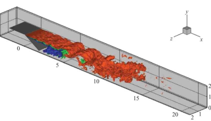
2 2 20 z x y 15 10 5 0 1 1 0
Figure 5. Instantaneous mixture-fraction iso-surfaces for Case A2. Iso-surfaces correspond to Z= 0.8 (red),Z= 0.5 (green) andZ= 0.2 (blue). Note the large spanwise-organized structures in the primary shear layer. Supplementary movies 1–3, available at journals.cambridge.org/flm, show animations of the mixture-fraction iso-surfaces for Cases A1–3, illustrating the unsteady flow characteristics and the effect of grid-resolution on the spatial structure of the flow.
5.3. Flow-field characteristics
The instantaneous mixture-fraction fields in figures 5 and 6 show spanwise-organized structures, similar to the ones observed in free-shear layers and the experiments of Johnson (2005) and Bergthorson et al. (2009). The primary shear layer appears more two-dimensional than the secondary because of the unsteady three-dimensional character of the flow in the recirculation region. The unsteady, complex nature of the flow is also illustrated in figure 7, where contours of the streamwise velocity corresponding to the mixture-fraction field of figure 6 are plotted. The recirculation region is comprised of several pockets of upstream-moving fluid, some of them not extending through the entire span. From the contour plots of instantaneous velocity and mixture-fraction fields, it appears that the large structures of the primary shear layer have a significant effect on the flow in the recirculation region. Supplementary movies 1–3, available with the online version of the paper, show an animation of the mixture-fraction field for the three resolutions used in Cases A1–A3, where the unsteady features of flow and resolution effects are better illustrated.
Before averages of the time-dependent flow fields are considered, the assumption of quasi-steady state is assessed. Improper boundary closures can result in a drift of mean quantities in the computational domain (Poinsot & Lele 1992), in which case statistics will not converge over time. For all the simulations performed, the average pressure andu-velocity on planes normal to the streamwise direction near the inflow of the top stream and the outflow were recorded as a function of time. In this manner, at least this aspect of the boundary closure is verified for this turbulent flow and the effect of the injection of the bottom stream through the ghost fluid is evaluated.
Figure 8 shows plane-averaged pressure at the inflow and outflow as a function of time. The pressure trace at the outflow fluctuates as a result of large-scale structures crossing the plane where the average is computed. As the structures exit the domain, they generate disturbances that travel upstream and exit through the inflow boundary. The upstream-travelling pressure waves are recorded in figure 8 as the fluctuations of the pressure trace at the inflow. Similar behaviour for free-shear layers has been
2 20 (a) 1 y 0 0 5 10 15 20 0 0.05 0.2 0.35 0.5 0.65 0.8 0.95 5 10 15 2 (b) z 1 z 0 x
Figure 6.Instantaneous mixture-fraction contours on the mid-span plane (a) and bottom
wall for Case A3. Black contour corresponds to the value of zero streamwise velocity. The flow is moving upstream in regions between the black contour and the bottom wall or when surrounded by the black contour. The correspondingu-velocity field is shown in figure 7.
2 (a) 1 y 0 20 0 –20 0 20 40 60 80 100120 5 10 x 15 20 0 5 10 15 2 (b) u (m s–1) 1 z 0
Figure 7.Instantaneous streamwise velocity contours on the mid-span plane (a) and bottom
wall for Case A3 at the same time as for the mixture-fraction field as in figure 6. Black contour corresponds to the value of zero streamwise velocity.
observed experimentally (Dimotakis & Brown 1976; Hall 1991) and is one of the factors that contribute to the generation of the instability of the primary shear layer. In order to remove the fluctuating part of the pressure traces, a rolling average is employed with a period of three convective times (Troll.ave.= 3tc). The flow
configuration, for the values of relatively small injection velocities studied, acts as a diffuser. The velocity profile at the outflow becomes more uniform compared with the inflow and the static pressure increases, as can be seen from the rolling averages of pressure in figure 8. The average outflow pressure remains constant with time at a value slightly above 105Pa. Note also that the average inflow pressure remains practically constant for the duration of the simulation after the short initial transient. 6. Grid-refinement study
Grid resolution, or the turbulence-resolution scale, is an important parameter in LES (Pope 2004a). For sufficiently refined calculations, a predictive LES model should yield turbulence statistics that are independent of grid resolution. Given that for a specific turbulence model and discretization the turbulence statistics exhibit good
t/tc Pressure (Pa) 0 5 10 15 20 96000 98000 100000 102000
Figure 8. Plane-averaged inflow and outflow pressure as a function of time for Case A2.
Thin lines denote pressure averaged over planes normal to the streamwise direction near the inflow and outflow. Outflow pressure is always higher than the inflow. Thick lines are a rolling average of the pressure traces with an averaging period of 3tc.
resolution independence, a secondary question is what are the necessary resolution requirements.
Resolution studies in LES can be comparisons of statistics with DNS data (e.g. Vreman, Geurts & Kuerten 1996; Meyers, Geurts & Baelmans 2003) or sensitivity studies with respect to grid-resolution (e.g. Stevens, Ackerman & Bretherton 2002; Bryan, Wyngaard & Fritsch 2003). The effect of numerical discretization errors and the interaction of such error with the modelling error have also been documented in these and other studies (Ghosal 1996; Vreman et al. 1996; Bryanet al. 2003). In the results reported here, the effect of grid spacing on the prediction of the mean fields and the mixture-fraction probability density functions is considered. Since a DNS is not feasible for the present flow, statistics are compared with respect to grid spacing and measurements from experiments.
It is expected that for relatively coarse resolutions, where a significant fraction of the turbulent motions and kinetic energy is not resolved, the modelling error is larger. As the grid is refined in a self-consistent LES–SGS scheme, the modelling error should become smaller. However, it may not continue to decrease with increasing resolution. Moreover, the behaviour of turbulence statistics as the grid is refined is expected to vary for different models and numerical discretizations (Pope 2004a).
Table 2 shows a comparison of the cell size with the Kolmogorov, λK, and Liepmann–Taylor, λT, (Dimotakis 2000) scales for the three cases of the refinement study. The Liepmann–Taylor scale is an estimate for the thickness of the internal laminar layers of the shear layer. The Kolmogorov and Liepmann–Taylor scales are estimated from the Reynolds number of the flow as defined in (5.1),
λK=hRe−3/4, (6.1)
and
λT= 5.0hRe−1/2. (6.2)
The coarsest simulation has grid cells that are almost 800 times larger than the smallest flow scales, while the grid cells at the finest resolution are 200 times larger than the smallest flow scales. In the highest resolution run, λT is of the order of the cell size. For all simulations, the SGS cutoff length is taken equal to the grid spacing.
Case A1 A2 A3 Re 3.8×10⁵ 3.8×10⁵ 3.8×10⁵ Number of cells 0.7×10⁶ 5.4×10⁶ 43.1×10⁶ x/ h 1/20 1/40 1/80 x/λK 770 385 192 x/λT 6.2 3.1 1.5
Table 2. Ratio of grid spacing to the Kolmogorov,λK, and Liepmann–Taylor scale,λT.
2 A1 y 1 0 0 0 0 5 10 15 20 0 5 10 15 20 0 5 10 x 15 20 2 A2 y 1 2 A3 y Z 1 0.05 0.2 0.35 0.5 0.65 0.8 0.95
Figure 9.Mean scalar fields for Cases A1–A3. Black contour corresponds to the value of zero
streamwise velocity, with flow moving upstream in regions between the black contour and the bottom wall. Case A1, the lowest resolution simulation, predicts a longer mean recirculation zone.
The computed mean quantities for Cases A1–A3 are different, with Case A1, the coarsest grid, exhibiting the largest variation between them, while Cases A2 and A3 agree well. The grid for Case A1 is too coarse to accurately capture the flow, a fact that is illustrated by the mean length of the recirculation region shown in figure 9. The mean reattachment point is 14 step heights downstream of the splitter plate in Case A1, whereas in Cases A2 and A3 it is at x= 9 and x= 8.5, respectively. The differences in the simulated mean flow fields yield different mixture-fraction fields as shown in figure 9.
Figure 10 provides a more detailed picture of the flow and supports the observation that mean profiles converge as the grid is refined, with Cases A2 and A3 in relatively good agreement with each other. Note that dependence on grid spacing of the profiles is not the same for all quantities. The streamwise velocity, u, is less sensitive than the mixture-fraction, Z, for example. As a consequence, agreement in u does not necessarily imply agreement in the meanZ, as can be seen for Cases A2 and A3 in figure 10.
In Appendix A, an analysis of mean profiles with respect to the length of the time interval over which the averaging is performed is carried out. The results of Appendix A indicate that the differences between grid resolutions cannot be
x = 4 x = 8 x = 16 u/U1 v/U1 y 0 0.5 1.0 u/U1 0 0.5 1.0 u/U1 0 0.5 1.0 0 0.5 1.0 1.5 2.0 0 0.5 1.0 1.5 2.0 0 0.5 1.0 1.5 2.0 (a) (b) (c) y 0 0.5 1.0 1.5 2.0 0 0.5 1.0 1.5 2.0 0 0.5 1.0 1.5 2.0 y 0 0.5 1.0 1.5 2.0 0.5 1.0 1.5 2.0 0.5 1.0 1.5 2.0 –0.04 –0.02 0 0.02 v/U1 –0.04 –0.02 0 0.02 v/U1 –0.04 –0.02 0 0.02 Z 0.2 0.4 0.6 0.8 1.0 0 0.2 0.4 0.6 0.8 1.0 Z 0 0.2 0.4 0.6 0.8 1.0 Z
Figure 10. Mean profiles for Cases A1–A3 at different streamwise locations, from (a) to (c) x= 4,8 and 16. Dash-dot lines correspond to Case A1, lowest resolution; dashed lines to Case A2, medium resolution; solid lines to Case A3, highest resolution.
attributed to variations attributable to insufficient convergence of the mean, but to differences resulting from grid resolution.
Turbulent kinetic energy profiles (TKE) are shown in figure 11. Atx= 4, the flow is essentially a free-shear layer of small thickness relative to the grid spacing. The total (resolved plus subgrid) TKE profile of the highest resolution case atx= 4 differs from the two other cases, suggesting that the primary shear layer near the origin may not be sufficiently resolved by grids A1 and A2. At the other two streamwise locations, TKE profiles can be seen to converge towards the profile of Case A3.
The ratio of the subgrid TKE, as estimated by the stretched vortex SGS model, to the total TKE is also shown in figure 11. At all three streamwise locations shown, the TKE ratio decreases monotonically with increasing resolution to less than 5 % for the finest resolution case.
The profiles in figures 9–11 indicate that Case A1 is under-resolved, even in an LES sense, whereas Cases A2 and A3 appear to capture the flow more accurately. This conclusion is also supported by the comparison to the experimental data discussed in §6.3. Accepting the results of Case A2 as sufficiently accurate, a criterion can be formulated for a resolution requirement for the current LES. Note that computational cost increases by a factor of 16 when the grid resolution is doubled. Using the information in figure 11, it can be inferred that a sufficiently resolved simulation requires a ratio of subgrid to total TKE of less than 20 %. This conclusion is in
x = 4 x = 8 x = 16 TKEtotal/1/2U12 y 0 0.05 0.10 TKEtotal/1/2U12 0 0.05 0.10 TKEtotal/1/2U12 0 0.05 0.10 0.5 1.0 1.5 2.0 y 0 0.5 1.0 1.5 2.0 y 0 0.5 1.0 1.5 2.0 0.5 1.0 1.5 2.0 0.5 1.0 1.5 2.0 0.5 1.0 1.5 2.0 0.5 1.0 1.5 2.0 (a) 0.5 1.0 1.5 2.0 (b) 0.5 1.0 1.5 2.0 (c)
TKESGS/TKEtotal
0.1 0.2 0.3 0.4 0
TKESGS/TKEtotal
0.05 0.10 0.15 0.20 0
TKESGS/TKEtotal
0.05 0.10
0.05 0.10 0.15 0.20 0 0.05 0.10
Z′SGS/Z′total
0.1 0.2 0.3 0.4 0
Z′SGS/Z′total Z′SGS/Z′total
Figure 11.Turbulent kinetic energy (subgrid plus resolved), ratio of turbulent kinetic energy
to subgrid turbulent kinetic energy and passive-scalar variance for Cases A1–A3 at different streamwise locations, from (a) to (c)x= 4, 8 and 16. Dash-dot lines correspond to Case A1, lowest resolution; dashed lines to Case A2, medium resolution; solid lines to Case A3, highest resolution.
agreement with LES resolution requirements discussed by Pope (2004b, §13.7). As a consequence ofSc= 1 in the LES, the same resolution requirement holds for passive mixing, i.e. a ratio of subgrid to total mixture-fraction variance less than 20 % for reliable prediction of mixing.
The fact that the ratio of subgrid to total TKE and mixture-fraction variance is estimated from the LES model and can vary for different SGS closures is a limitation of the analysis. DNS data or measurements can be used to overcome this limitation. However, simulations and measurements present severe challenges in complex high-Reynolds-number flows. Despite this limitation, the process of model validation can help reduce and quantify the uncertainties associated with estimates of subgrid quantities. In a comparison of turbulence statistics corrected for the subgrid contribution, Pantanoet al.(2008) reported good agreement in an LES of a turbulent wall-bounded flow with the corresponding DNS data using the stretched-vortex model.
Because of the underlying modelling assumptions in LES, it is expected that a prerequisite for this criterion is the resolution of all significant flow features, such as relatively thin turbulent interfaces encountered in strongly stably stratified flows and
features that are directly generated by the boundary conditions of the problem. The resolution criterion discussed here implies that the accuracy of the LES prediction becomes independent of the size of the smallest scale in the flow provided a minimum fraction of the TKE is resolved.
6.1. Mixture-fraction probability density functions
Mixture-fraction p.d.f.s contain the full single-point statistical information of Z(t, x, y, z). The passive-scalar p.d.f.,P(Z;x, y), can be used to obtain expectations of quantities that depend on mixture fraction such as the chemical product fraction and the temperature rise, or be directly used to study the characteristics of mixing.
Unfortunately, the actual p.d.f. cannot be constructed from the resolved fields of the LES alone because the value ofZin each cell represents only the volume average, yielding only the first (mean) and zeroth (normalization) moments of the passive-scalar p.d.f. Additional information about the subgrid p.d.f. is required. In estimating the total (resolved-scale plus contribution from subgrid scales) p.d.f., one approach is to assume a functional form of the SGS scalar distribution and match the low-order statistics that are available from the resolved field (e.g. Williams 1985; Peters 2000). This is called the presumed-shape p.d.f. approach.
One of the most widely used distributions for the SGS p.d.f. is the beta distribution (Cook & Riley 1994; Jim´enez et al. 1997). For the construction of the total p.d.f., it is assumed that, independent of location in the flow, the subgrid p.d.f. can be approximated by a beta distribution. The mixture-fraction mean and variance, as estimated by the SGS model in each grid cell, are used to parameterize the SGS distribution.
The procedure of computing the total p.d.f. follows Hill, Pantano & Pullin (2006). The resolved-scale p.d.f. is the (normalized) histogram ofZ realizations. As with the computation of mean quantities, p.d.f.s are functions of x andy, and realizations in span and time at (x, y) are used to constructP(Z; x, y). The SGS p.d.f.,Psgs(Z, t,x), is formally defined as the Favre-p.d.f. of Z (Bilger 1975, 1977), such that for any functionf(Z),
f(Z, t,x) =
f(Z)Psgs(Z, t,x) dZ. (6.3) The relationship between the total and subgrid p.d.f. is further discussed by Gao & O’Brien (1993) and Hill et al.(2006).
Although the filtered scalar equation (4.6) must, ideally, observe the boundedness of the scalar field, 06Z61, as does the exact scalar-transport equation (e.g. Dimotakis & Miller 1990), the approximation of the subgrid scalar flux and the numerical discretization do not preclude the generation of scalar values outside the interval [0,1]. This is found to be the case for the present simulations. While the observed scalar out-of-bounds excursions occupy a small fraction of the volume, they are unphysical and the result of modelling error. Because the out-of-bounds scalar excursions do not occur uniformly in the computational domain, ignoring the problematic values would introduce a normalization error and bias in the statistics. Therefore, scalar valuesZ <0 andZ >1 were placed in the smallest and largest bins, respectively, preserving probability normalization. Further details and statistics of the excursions are provided in Appendix B.
Each panel of figure 12 shows p.d.f.s along the transverse direction for Case A3 at fixedx. In these plots, they axis is the transverse coordinate. Any constant-ytransect corresponds toP(Z;x, y).
x = 4 2.0 (a) 1.5 y1.0 0.5 0 0.2 0.4 0.6 0.8 1.0 0 0.2 1 3.25 5.5 7.75 10 0.4 0.6 0.8 1.0 0.2 0.4 0.6 0.8 1.0 2.0 (b) Z Z Z 1.5 1.0 0.5 2.0 (c) 1.5 1.0 0.5 0 x = 8 x = 16 p.d.f.
Figure 12.Mixture-fraction p.d.f.s for Case A3 at different streamwise locations. Each panel
shows p.d.f.s along the transverse direction. Grey-scale contours correspond to the total p.d.f. whereas black contours to the resolved-scale. Both contour sets have identical increments. The differences between the total and resolved-scale p.d.f.s were found to be small for all cases simulated.
In all simulations performed, the difference between the resolved-scale and total p.d.f.s was found to be small and traceable to the small values of subgrid variance predicted by the LES model (see also figure 11).
The characteristics of the p.d.f.s change with the streamwise coordinate. Atx= 4, the effect of the recirculation zone results in distributions of mixed fluid near the bottom wall (y= 0). With increasing y, there is a region where mostly pure bottom-stream fluid (Z= 0) is found (see figure 9), while for larger y only pure top-stream fluid is present. All low-speed fluid (initially,Z= 0) has been mixed byx = 8.
The p.d.f.s atx= 8, the approximate location of mean reattachment, show that the mixture becomes more homogeneous near the bottom wall than at the centre of the duct, with the most probable value moving towards lower values ofZ for increasing y. This can be attributed to the fact that, as seen in figure 9, pure bottom-stream fluid, although not present near the bottom wall, can be found aty= 0.5 up tox= 4. Moreover, fluid near the bottom wall in the recirculation zone is moving at low speeds, resulting in larger Lagrangian times for fluid elements that allow the mixture to become more homogeneous.
Downstream of the mean reattachment, atx= 16, pure top-stream fluid occupies a small fraction of the height while the p.d.f.s appear more narrow with larger means.
6.2. Velocity and mixture-fraction spectra
Two types of spectra were computed: spatial spectra along the statistically homogeneous spanwise direction and temporal spectra using time traces at fixed locations in space.
Spatial one-dimensional spectra for the three components of velocity and mixture fraction are shown in figures 13 and 14. The spectra were calculated by taking the ensemble average of one-dimensional spectra for many flow realizations. The results for the medium resolution Case A2 show effects of aliasing at the highest wavenumbers. Aliasing is found to decrease considerably for the high-resolution Case A3, with the exception of the spanwise velocity spectrum (figure 14). Aliasing in the one-dimensional spectrum of the velocity component in the direction of the transform is commonly observed in different flows and can be attributed to the
k3 EZ 101 102 103 104 10–1 (a) (b) 10–2 10–3 10–4 10–5 10–6 10–7 10–8 10–1 10–3 k3 101 102 103 104 10–2 ~k–5/3 ~k–5/3 y = 0.6 y = 1.0 y = 0.2 y = 0.6 y = 1.0 y = 0.2 Eu 104 103 102 101 100
Figure 13. One-dimensional mixture-fraction (a) and streamwise velocity spectra at x= 6.
Spectra were computed along the statistically homogeneous spanwise direction. Solid lines correspond to Case A3 and dashed lines to Case A2. Three sets of spectra are shown at
y= 0.2, 0.6 and 1. For clarity, the spectra aty= 0.6 and y= 1 were shifted upwards by one and two decades, respectively.
k3 Ev Ew 101 102 103 104 102 101 100 10–1 10–2 10–3 ~k–5/3
Figure 14. One-dimensionalv-velocity (solid line) andw-velocity spectra atx= 6 andy= 6. implementation of the stretched-vortex model and numerical method, which remain current topics of research.
Temporal mixture-fraction spectra are shown in figure 15. The time trace records were windowed using a 25 % cosine taper (Tukey) window (Harris 1978), since the trace is not periodic. The resulting spectra were subsequently smoothed using a one-third octave Gaussian filter. The time traces are well resolved in time compared with the spatial fields, as a result of the small time steps in the LES because of the CFL condition requirement. This difference is responsible for the observed difference in behaviour between the temporal and spatial spectra at high wavenumbers.
6.3. Comparison with experimental data
Results from Cases A1–A3 are compared against the measurements reported by Johnson (2005). The bottom-stream velocity in Cases A1–A3 corresponds to the case U2= 11 m s−1of Johnson (2005). The comparison is in terms of the pressure coefficient along the bottom and top guide walls, the temperature rise for two equivalence ratios and the probability of mixed fluid. Since heat release effects are small and neglected in the simulations, pressure-coefficient data are compared with those of non-reacting
ω EZ 101 102 103 104 105 106 ω 101 102 103 104 105 106 10–4 (a) (b) 10–5 10–6 10–7 10–8 10–9 10–10 10–10 10–4 10–5 10–6 10–7 10–8 10–9 ~k–5/3
Figure 15.Temporal mixture-fraction spectra at mid-span and x= 6. (a) Spectra at y= 0.2
(dashed-dot line), y= 0.6 (dashed line) and y= 1 (solid line). (b) The difference between the raw and smoothed spectrum.
x Cp 0 5 10 15 20 –0.1 0 0.1 0.2 0.3 0.4
Figure 16.Comparison of pressure coefficient along the bottom (solid line, filled circles) and
top (dashed line, open circles) guide walls. Lines correspond to Case A3 of the simulations and circles to the experiments of Johnson (2005).
experiments and the mixing to low-heat release chemically reacting flow cases. The pressure coefficient, a non-dimensional measure of pressure recovery, is defined as
Cp = p−p1 1 2ρ1U 2 1 . (6.4)
Quantities with subscript 1 correspond to top-stream means atx= 0.
The pressure coefficient comparison is shown in figure 16. The agreement between the predicted flow and the measured is satisfactory with two main differences. The pressure coefficient in the simulation is positive throughout the computational domain, whereas in the experiment the flow appears to accelerate downstream of the splitter plate before recovering pressure after the reattachment of the primary shear layer. This may occur because of the different shape or position of the primary shear layer. The second and most important difference is the length of the recirculation zone. In the experiments, the mean length is about one step height less than the simulation, a trend observed in all simulations. This can be explained by a mismatch in the virtual origin of the primary shear layer between the experiments and simulations. In the LES, the shear layer does not develop three-dimensional fluctuations until some distance downstream of the splitter plate, owing to the length needed for instabilities
φ = 1/8 φ = 8 ΔT/ΔTf y 0 0.2 0.4 0.6 0.8 1.0 ΔT/ΔTf 0 0.2 0.4 0.6 0.8 1.0 0 0.2 0.4 0.6 0.8 1.0 0.5 1.0 1.5 2.0 0.5 1.0 1.5 2.0 0.5 1.0 1.5 2.0 (a) (b) (c) Pm
Figure 17. Comparison of normalized temperature rise for H2 rich (φ= 1/8) and F2 rich
(φ= 8) and probability of mixed fluid atx= 7.8. Case A1: dashed-dot lines; Case A2: dashed lines; Case A3: continuous lines; Symbols: experimental measurements.
to develop. On the other hand, in the experiments, the (initial) state of the shear layer is quite different when it separates from the splitter plate. The fluctuations in the boundary layer upstream of the splitter plate, the separation of the flow at the top of the inclined ramp and the effect of the jets emanating from the perforations of the ramp contribute to a different initial condition for the shear layer. Previous studies have shown that growth rate in free-shear layers is sensitive to inflow conditions (e.g. George 1989; Slessor et al. 1998). These effects are not modelled in current simulations and, as a consequence, the virtual origin and growth rate are expected to differ from the experiments. Unlike simulations of free-shear layers and jets, the virtual origin is not a free parameter here because the origin of the secondary shear layer is fixed by the experimental geometry.
The p.d.f.s of mixture fraction are used to estimate the temperature rise. At a particular mixture fraction, the relative amount of product is given by
Yp(Z;Zφ) = ⎧ ⎪ ⎪ ⎨ ⎪ ⎪ ⎩ Z Zφ for 06Z6Zφ, 1−Z 1−Zφ for Zφ 6Z61, (6.5)
assuming complete consumption of the lean reactant. At the stoichiometric mole fraction,
Zφ=
φ
φ+ 1, (6.6)
reactants are completely consumed, whereφis the stoichiometric mixture ratio defined as the volume (number of moles) of high-speed fluid that carries sufficient reactants to completely consume a unit volume (mole) of low-speed fluid (Dimotakis 1991).
The temperature rise normalized by the adiabatic flame temperature rise,Tf, can
then be computed by T(y;φ) Tf = 1 0 Yp(Z, Zφ)P(Z;y) dZ. (6.7)
Figure 17 shows the comparison of the normalized temperature rise for H2-rich (φ= 1/8) and F2-rich (φ= 8) conditions atx= 7.8.
The probability of mixed fluid is defined as the integral of the mixture-fraction p.d.f. ignoring the contribution from the values near Z= 0 andZ= 1 that correspond to