1
IMPEDANCE MEASURING SYSTEM BASED ON A DSPIC
José Santos
1, Pedro M. Ramos
21IST, UTL, Lisbon, Portugal, [email protected]
2Instituto de Telecomunicações, DEEC, IST, UTL, Lisbon, Portugal, [email protected]
Abstract - This paper describes a device based on a dsPIC (Digital Signal Peripheral Interface Controller) as a processing unit, capable of making impedance measurements at multiple frequencies. A DDS (Direct Digital Synthesizer) stimulates the measurement circuit composed by the reference impedance and the unknown impedance. The voltage across the impedances is amplified by programmable gain instrumentation amplifiers and then digitized by analog to digital converters. To measure the impedance, a seven-parameter sine-fitting algorithm is used to estimate the sine signals across the impedances. The dsPIC is connected through RS-232 to a computer where the user can view the measurement results.
Keywords: Impedance measurement, dsPIC, ADC, Sine-fitting.
I. INTRODUCTION
As the world of technology evolves, so does its need for improved measurement techniques. One of the major areas of investigation that has been growing for the past few years is impedance measurement. With a wide spectrum of applications, from medicine to electronics, impedance measurement is surely an area worth researching.
In the field of medicine, impedance measurement can be used in electrical impedance myography (EIM), which is a non-invasive technique for neuromuscular assessment [1, 2]. It enables the detection of degenerative neuromuscular diseases.
Impedance measurement can also play an important part in civil engineering. It can be used to measure the level of corrosion in some materials such as reinforced steel in concrete [3]. A concrete Surface-based Measurement Method (SMM) is used as nondestructive technique to determine the deterioration of structures and study the corrosion process. The method is able to determine the corrosion state of the reinforcing bars, as well as the resistivity of the concrete itself, from the concrete surface and with no need of connection to the reinforcement.
The technological advances of the past few years have improved the performance of data acquisition systems to a point where it is possible to implement cheaper ways to make the same measurements as dedicated expensive equipment, without relevant degradation of the system accuracy.
The continuous improvement in performance of new devices, such as Analog to Digital Converters (ADCs),
combined with more powerful signal processing techniques, are some of the factors that have contributed to this fact.
Typical measuring techniques/instruments are either too costly, or don’t have enough accuracy and have a reduced frequency range. Agilent Technologies is one of the leading companies for measurement systems. Its simplest impedance measuring system [4] covers frequencies from 40 Hz up to 110 MHz with a basic accuracy of 0.08 %. However, its price of nearly 30.000€ makes the system well beyond the budget capabilities of many companies and research institutes.
Therefore there has been an increasing demand for low cost impedance measuring systems capable of performing measurements at a broad range of frequencies but still with comparable accuracy to that of sophisticated impedance measurement equipment.
This work seeks to develop, implement and characterize a low-cost device capable of measuring impedances at a wide range of frequencies by using ADCs and a dsPIC as a central processing unit to both control all the necessary hardware of the measuring circuit and run the sine fitting algorithm necessary to the proper measurement of the impedance. A personal computer is also used, which acts as interface between the user and the device, allowing the monitoring of the acquired samples.
The device has to be able to measure impedances in the frequency range from 500 Hz to 200 kHz. The amplitude of the impedances to be measured is intended to be between 100 Ω and 10 kΩ.
The dsPIC is responsible for: i) controlling the stimulus module of the measurement circuit through a DDS which is responsible for generating the sine signal with the measurement frequency; ii) controlling the programmable gain instrumentation amplifiers (PGIAs) that amplify the voltage at the terminals of the two impedances (reference impedance and impedance under measurement); iii) controlling and communicating with the ADCs responsible for the digitalization of the output voltage from the PGIAs; iv) applying the algorithm to determine the amplitudes and phases of the sinusoidal signals across each impedance (sine-fitting); v) applying the algorithms to correct systematic errors; vi) transmitting the results to a PC (Personal Computer) through a RS-232 connection.
2
In the end the user will be able to control the device in order to decide at which frequency he wants to perform the impedance measurement.II. SYSTEM’S ARCHITECTURE
A. Measurement Circuit and Method
Several impedance measurement methods exist. Traditional methods include: bridge, resonant, I-V or volt-ampere, RF I-V, network analysis and auto balancing bridge [5].
The measurement method used in this work is based in the volt-ampere method [5] and it is similar to that in [6], but in this case a dsPIC is used as a processing unit and a DDS is used to inject current in the circuit.
The impedance measurement circuit used in this work to ascertain the value of the unknown impedance is presented in Fig. 1.
Fig. 1 - Measurement circuit. is the impedance under measurement and is the reference impedance.
The measurement procedure is done according to the following steps:
(i) The dsPIC controls the DDS in order to generate a sine wave with the user-defined measurement frequency.
(ii) The dsPIC selects the gains of the amplifiers according to the magnitudes of the signals across the reference impedance and the impedance under measurement.
(iii) The dsPIC controls the ADCs to acquire simultaneously the samples (in this case 1024 per channel) of the output voltage of the PGIAs, which amplify the signals across the reference impedance (PGIA 1) and the unknown impedance (PGIA 2). The gains of both amplifiers are set by the dsPIC to maximize the amplitudes of the signals, but with care to avoid saturation of the digitizing channels. (iv) A seven parameter sine-fitting algorithm is applied
in order to determine the amplitudes and phases
of the sine waves that best fit the acquired samples of both channels ( ).
(v) The modulus and phase angle of the impedance under measurement are calculated by
Once all the calculations are done, the experimental results of the measurement are transmitted to the PC.
B. Devices Used in the Circuit
The processing unit used in the system is a 16-bit dsPIC33FJ256GP710 microcontroller from Microchip. It has a throughput up to 40 MIPS, 256 kB of flash program memory and 30 kB of RAM (Random Access Memory). The dsPIC is connected to the Explorer 16 Development Board from Microchip which is used as a prototyping tool to help implement the system.
The DDS module used to stimulate the measurement circuit is the AD9833 from Analog Devices, which produces the sine signal with the desired measurement frequency. The AD9833 is capable of producing sine, triangle and square waveforms with an output frequency range from 0 MHz to 12.5 MHz, and the amplitude of the output signal is typically 0.6 Vpp. The module is also compatible with SPI (Serial Peripheral Interface) protocol, allowing its control by a microcontroller, in this case the dsPIC.
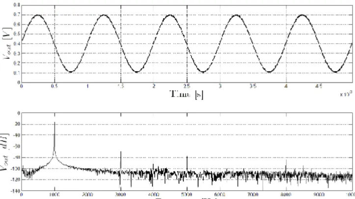
The DDS output sine signal with a frequency of 1 kHz and the correspondent FFT is presented in Fig. 2.
Fig. 2 - Output signal and correspondent FFT from the DDS at 1 kHz.
The signal was measured through an Agilent 54622D Mixed Signal Oscilloscope from Agilent Technologies. Two million samples of the signal were acquired and transferred to
3
a computer where they were processed in the MATLAB environment to obtain the sine signal and its correspondent FFT (Fast Fourier Transform) presented in Fig. 2. The Total Harmonic Distortion (THD) of the signal was also estimated: 51.175365 dB.In this work an AD8250 PGIA from Analog Devices was used. It allows four programmable gains: 1, 2, 5 and 10. The gain is digitally set by the processing unit in order to maximize the voltages at the ADCs inputs, while avoiding saturation of the digitizing channels. This is done in order to obtain a better resolution of the acquired signals.
The two ADCs used were external to the dsPIC. These ADCs are the AD7980 from Analog Devices. The AD7980 is a successive approximation converter with 16-bit resolution and conversion speeds up to 1 MS/s. The AD7980 has the ability to daisy-chain several ADCs on a single data bus.
The sampling frequency of the two ADCs is controlled by the dsPIC through the SPI interface. In order to be possible to use the ADCs maximum conversion speed of 1 MS/s and read the samples of both ADCs (32 bits), it would be necessary an SPI module with at least an operating frequency of 32 MHz, however at the dsPIC’s maximum throughput, 40 MIPS, the SPI module can only operate at a maximum frequency of 10 MHz, and so the maximum sampling frequency possible for this work was greatly reduced. It can attain the maximum value of 178 kS/s.
III. ALGORITHMS
A. Selection of Sampling Frequency
The range of frequencies used in this work goes from 500 Hz to 200 kHz. Since the maximum sampling frequency (FSmax) is 178 kS/s, two cases must be considered for the
acquisition of the signals: the case with no under sampling and the case with under sampling.
In the case with no under sampling, the sampling frequency is chosen in way that allows the acquisition of at least eight periods of the signals.
In the case with under sampling the sampling frequency is chosen according to
where F is the measurement frequency, FS is the selected
sampling frequency, mreal is the number of full folds of the
signal spectrum and mideal is the desired number of folds of
the signal spectrum. The mideal value is chosen in a way that
the acquired signal’s frequency (apparent) will be at the middle of the spectrum, which corresponds to the best case.
B. Three-Parameter Sine-Fitting
The three-parameter sine-fitting algorithm is a non-iterative algorithm that, with the knowledge of the frequency, estimates the amplitude, the phase and the DC component of the acquired sine signal [7].
The acquired sine signals can be represented by
or by with and
where is the amplitude, is the phase and is the DC component of the signal.
The estimated parameter vector is
where is the sample vector
and
N is the number of samples acquired, and is the pseudo inverse matrix of .
The frequency for the three-parameter algorithm was estimated using the FFT and the IpDFT (Interpolated Discrete Fourier Transform) [8] algorithms.
C. Selection of Reference Impedance and PGIAs Gains
The algorithm selects the reference impedance that best matches the magnitude of the impedance under measurement. This is done in order to ensure that the amplitude of the acquired signals is as close as possible to the ADC input range. This way it is possible to maximize the use of the ADC dynamic range. In order to choose the proper reference impedance, it is necessary to perform an initial acquisition and estimate the amplitude of the unknown impedance by resorting to the three-parameter sine fitting algorithm.
4
This algorithm also digitally controls the gains of the PGIAs to have the maximum voltage possible at each ADC input channel in order to obtain a better resolution of the acquired signals across the reference impedance and the impedance under measurement.Given the magnitude of the signals, obtained with the three-parameter sine fitting algorithm, the algorithm determines whether it is possible or not to increase the gains of each amplifier and if so how much. The gains are set according to the values admitted by the amplifiers and in a way that does not exceed the input range of the ADCs.
The reference impedances used in this work were resistors with a tolerance of ±5%. They were characterized using a 3522-50 LCR HiTESTER from HIOKI, to measure the reference impedances in the frequency range from 100 Hz to 100 kHz with 100 Hz intervals. Once the measurements were done, the results were processed in the MATLAB environment to estimate the resistance value (R) that best adapts to the measured values. For this purpose it was used the fminsearch function. This function minimizes the errors between the measured values and the estimated R value, thus obtaining the optimum value for R. Table I presents the estimated R values.
Table I - Estimated R values. Reference
Impedance (Ω) Estimated R Values (Ω) Error
120 118.255608 1.564026 × 10⁻⁶ 220 216.015079 7.630637 × 10⁻⁵ 510 502.384931 2.214254 × 10⁻⁶ 1200 1182.838493 4.618403 × 10⁻⁵ 2200 2161.503298 3.286041 × 10⁻⁶ 5100 5040.373694 3.221815 × 10⁻⁵
The value used for the phase of the reference impedances is zero.
D. Seven-Parameter Sine-Fitting
The seven-parameter sine-fitting algorithm is an iterative algorithm which uses the acquired data from two channels with the same frequency to estimate the amplitude, phase and DC component of both signals, plus their common frequency [9].
Just like in the case of the three-parameter algorithm, the sine signals of each channel can be represented by (6) or by (7) considering the relations in (8) and (9). Since the initial estimates of the parameters are crucial for the algorithm to converge, these values were obtained through the three-parameter sine-fitting.
The algorithm is described in detail in [9].
The iterative process of the algorithm ends when the relative frequency adjustment is below a preset threshold, which is set to in the case of this work. is the frequency correction that updates the estimated common frequency.
With the estimated parameters of this algorithm it is possible to determine the unknown impedance.
IV. SYSTEM’S CONTROL SOFTWARE
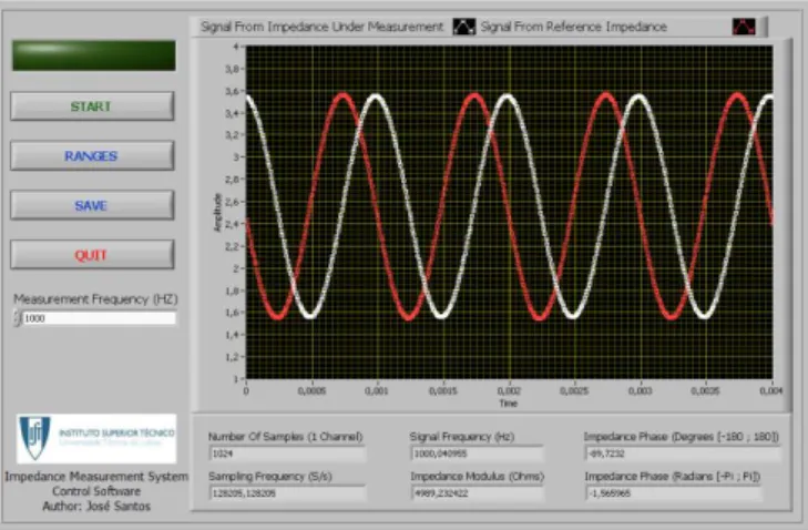
It was implemented a control software which runs in a PC. The software acts as an interface between the user and the device, giving its user the means to interact with it. This software allows the user to choose the frequency at which to perform the measurement of the unknown impedance. Another feature of the software is the ability to communicate with the device in order to obtain information regarding the device’s maximum operating ranges. An important aspect of the software is the fact that it allows the user to view and interpret the acquired samples of the measurements done.
The software was developed in the LabVIEW environment, which provides simple and intuitive programming tools to implement even the most complex program, and also has the capability to easily create an application that can run in a PC, even if it does not have the LabVIEW environment installed.
The main window of the implemented software is represented in Fig. 3.
5
V. EXPERIMENTAL RESULTSThe experimental results regarding the measurement of different impedances are presented. Ten impedances with different amplitudes in the range from 100 Ω to 10 kΩ, and phases in the range from -90º to 90º were tested at 1 kHz and the results are compared to those obtained with the 3522-50 LCR HiTESTER from HIOKI.
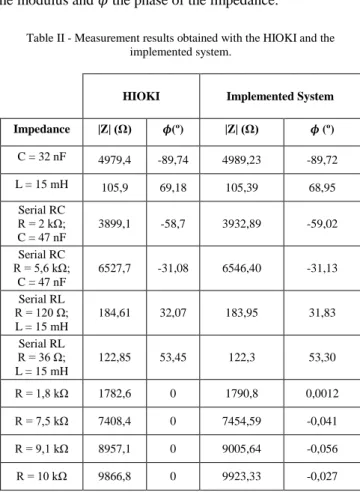
The measurement results are presented in Table II. |Z| is the modulus and the phase of the impedance.
Table II - Measurement results obtained with the HIOKI and the implemented system.
HIOKI Implemented System
Impedance |Z| (Ω) (º) |Z| (Ω) (º) C = 32 nF 4979,4 -89,74 4989,23 -89,72 L = 15 mH 105,9 69,18 105,39 68,95 Serial RC R = 2 kΩ; C = 47 nF 3899,1 -58,7 3932,89 -59,02 Serial RC R = 5,6 kΩ; C = 47 nF 6527,7 -31,08 6546,40 -31,13 Serial RL R = 120 Ω; L = 15 mH 184,61 32,07 183,95 31,83 Serial RL R = 36 Ω; L = 15 mH 122,85 53,45 122,3 53,30 R = 1,8 kΩ 1782,6 0 1790,8 0,0012 R = 7,5 kΩ 7408,4 0 7454,59 -0,041 R = 9,1 kΩ 8957,1 0 9005,64 -0,056 R = 10 kΩ 9866,8 0 9923,33 -0,027
As shown in Table II, the experimental results obtained with the implemented system are quite close to those obtained with the HIOKI, demonstrating that it is possible to implement a low-cost impedance measurement device with comparable accuracy of that of sophisticated measurement equipment.
VI. CONCLUSIONS
Given the high cost of sophisticated equipment dedicated to impedance measurement, it is important to develop new and cheaper ways to make the same type of measurements at a more reduced cost.
The measurement setup proposed in this work is an attempt to do just that. It uses a number of low cost equipment, which by operating together can produce results
with comparable accuracy to those obtained with dedicated measurement equipment. This is possible because of the great processing capability of the processing unit used, the dsPIC, combined with the powerful signal processing techniques applied, the three-parameter sine fitting algorithm and the seven-parameter sine fitting algorithm.
The implemented system facilitates the interaction with its user, since it is possible to connect it to a PC, through a RS-232 connection, to receive commands from the user and allow him to monitor the device and save the results of the measurements done.
The implemented system operates in a wide frequency range, 500 Hz to 200 kHz, and is capable of measuring impedances in the amplitude range from 100 Ω to 10 kΩ.
To operate in this frequency range it was necessary to apply under sampling techniques because of the constraints imposed by the dsPIC in terms of maximum sampling frequency.
The experimental results produced in this work were compared with a commercially available device, the 3522-50 LCR HiTESTER from HIOKI, by measuring ten different impedances in the amplitude range from 100 Ω to 10 kΩ and in the phase range from -90º to 90º at a measurement frequency of 1 kHz. Given the experimental results presented, it was demonstrated that it is possible to implement a low-cost device operating at a wide frequency range, but still with measurement accuracy comparable to that of sophisticated high-cost dedicated impedance measurement systems.
VII. REFERENCES
[1] Olumuyiwa T. Ogunnika, Michael Scharfstein, Roshni C. Cooper, Hongshen Ma, Joel L. Dawson and Seward B. Rutkove, “A Handheld Electrical Impedance Myography Probe for the Assessment of Neuromuscular Disease”, 30th Annual International IEEE EMBS Conference, Vancouver, British Columbia, Canada, August 20-24, 2008.
[2] Michael Scharfstein, “A Reconfigurable Electrode Array for Use in Rotational Electrical Impedance Myography”,
Thesis for the Degree of Master of Engineering in Electrical Engineering and Computer Science, Massachusetts Institute of Technology, September 2007. [3] M. Mancio, J. Zhang and P.J.M. Monteiro,
“Nondestructive surface measurement of corrosion of reinforcing steel in concrete”, Canadian Civil Engineer, v. 21, no. 2, pp. 12-14, May 2004.
[4] Agilent 4294A Precision Impedance Analyzer, Data Sheet, available at www.agilent.com April 2008.
6
[5] The Impedance Measurement Handbook – A Guide toMeasurement Technologies and Techniques, Agilent Technologies Co., 2000.
[6] Pedro M. Ramos, Fernando M. Janeiro, Mouhaydine Tlemçani and A. Cruz Serra, “Recent Developments on Impedance Measurements With DSP-Based Ellipse-Fitting Algorithms”, IEEE Transactions on Instrumentation and Measurement, vol. 58, no. 5, May 2009.
[7] IEEE Std. 1057-1994, Standard for Digitizing Waveform Records, The Institute of Electrical and Electronics Engineers, New York, December 1994.
[8] Tamás Zoltán Bilau, Tamás Megyeri, Attila Sárhegyi, János Márkus, István Kollár, “Four Parameter Fitting Of Sine Wave Testing Result: Iteration and Convergence”,
Computer Standards and Interfaces, Vol. 26, pp. 51-56, 2004.
[9] Pedro M. Ramos, Fernando M. Janeiro, Tomáš Radil, “Comparison of Impedance Measurements in a DSP using Ellipse-fit and Seven-Parameter Sine-fit Algorithms”, Elsevier Editorial System(tm) for Measurement, 2009.