Separating Models of Learning from Correlated and Uncorrelated Data

Separating Models of Learning from

Correlated and Uncorrelated Data

Ariel Elbaz [email protected]

Homin K. Lee [email protected]

Rocco A. Servedio∗ [email protected]

Andrew Wan [email protected]

Department of Computer Science Columbia University

NY, NY 10027, USA

Editors: Peter Auer and Ron Meir

Abstract

We consider a natural framework of learning from correlated data, in which successive examples used for learning are generated according to a random walk over the space of possible examples. A recent paper by Bshouty et al. (2003) shows that the class of polynomial-size DNF formulas is efficiently learnable in this random walk model; this result suggests that the Random Walk model is more powerful than comparable standard models of learning from independent examples, in which similarly efficient DNF learning algorithms are not known. We give strong evidence that the Random Walk model is indeed more powerful than the standard model, by showing that if any cryptographic one-way function exists (a universally held belief in cryptography), then there is a class of functions that can be learned efficiently in the Random Walk setting but not in the standard setting where all examples are independent.

Keywords: random walks, uniform distribution learning, cryptographic hardness, correlated data, PAC learning

1. Introduction

It is a commonly held belief in machine learning that having access to correlated data—for example, having random data points that differ only slightly from each other—is advantageous for learning. Thus it is a natural research goal to rigorously validate this belief from the vantage point of the abilities and limitations of computationally efficient learning.

We study a natural model of learning from correlated data, by considering a framework in which the learning algorithm has access to successive examples that are generated by a random

walk. We give strong evidence that learning is indeed easier, at least for some problems, in this

framework of correlated examples than in the standard framework in which no correlations exist between successive examples.

1.1 Background

In the well-known Probably Approximately Correct (PAC) learning model introduced by Valiant (1984), a learning algorithm is given access to a source EX_D(c)of labeled examples each of which is drawn independently from a fixed probability distribution

D

over the space of possible instances. The goal of the learning algorithm is to construct (with high probability) a high-accuracy hypothesis for the target concept c with respect to

D

.

Aldous and Vazirani (1990) introduced and studied a variant of the PAC learning model in which successive examples are generated according to a Markov process, that is, by taking a random walk on an (exponentially large) graph. Subsequent work by Gamarnik (1999) extended this study to infinite Markov chains and gave bounds on the sample complexity required for learning in terms of the VC dimension and certain mixing properties of the underlying Markov chain. Neither Aldous and Vazirani (1990) nor Gamarnik (1999) considered computational issues for learning algorithms in the Random Walk framework.

In this paper we consider an elegant model of learning from Random Walk examples that is well suited for computational analyses. This model was introduced by Bartlett et al. (2002) and subse-quently studied by Bshouty et al. (2003) and Roch (2006). In this framework (described in detail in Section 2), successive examples for the learning algorithm are produced sequentially according to an unbiased random walk on the Boolean hypercube_{0,1_}n. The PAC goal of constructing a high-accuracy hypothesis for the target concept with high probability (where high-accuracy is measured with respect to the stationary distribution of the random walk, that is, the uniform distribution on_{0,1_}n) is unchanged. This is a natural way of augmenting the model of uniform distribution PAC learn-ing over the Boolean hypercube (which has been extensively studied, see, for example, Blum et al. 1994; Bshouty et al. 1999; Bshouty and Tamon 1996; Jackson 1997; Jackson et al. 2002; Kharitonov 1993; Linial et al. 1993; Verbeurgt 1990 and references therein) with the ability to exploit correlated data.

Bartlett et al. gave polynomial-time learning algorithms in this model for several concept classes including Boolean threshold functions in which each weight is either 0 or 1, parities of two mono-tone conjunctions over x1, . . . ,xn, and Disjunctive Normal Form (DNF) formulas with two terms.

These learning algorithms are proper, meaning that in each case the learning algorithm constructs a hypothesis representation that belongs to the class being learned. Since proper learning algorithms were not known for these concept classes in the standard uniform distribution model, this gave the first evidence that having access to random walk examples rather than uniform independent exam-ples might bestow a computational advantage.

More recently, Bshouty et al. (2003) gave a polynomial-time algorithm for learning the unre-stricted class of all polynomial-size DNF formulas over_{0,1_}n in the Random Walk model. Since no comparable polynomial-time algorithms are known in the standard uniform distribution model— and their existence is a well-studied open question for which an affirmative answer would yield a $1000 prize (see Blum, 2003)—this gives stronger evidence that the Random Walk model is strictly more powerful than the normal uniform distribution model. Thus, it is natural to now ask whether the superiority of random walk learning over uniform distribution learning can be established under some widely accepted hypothesis about efficient computation.

models, as well as in far weaker models, by an algorithm that nondeterministically “guesses” a cir-cuit and then checks consistency with a polynomial-size sample. Thus without some computational hardness assumption, essentially all considerations about the computational complexity of learning would become trivial.)

1.2 Our Results

In this work we give a separation, under a generic cryptographic hardness assumption, between the Random Walk model and the uniform distribution model. Our main result is a proof of the following theorem:

Theorem 1 If any cryptographic one-way function exists, then there is a concept class over_{0,1_}n

that is PAC learnable in poly(n)time in the Random Walk model but is not PAC learnable in poly(n)

time in the standard uniform distribution model.

We emphasize that the separation established by Theorem 1 is computational rather than information-theoretic. It will be evident from our construction that the concept class of Theorem 1 has poly(n)

VC dimension, and thus the class can be learned using poly(n)many examples even in the distribution-independent PAC learning model; the difficulty is in obtaining a polynomial-time algorithm.

We remind the reader that while the existence of any one-way function is a stronger assumption than the assumption that P₆=NP (since at this point it is conceivable that P₆=NP but one-way func-tions do not exist), it is an almost universally accepted assumption in cryptography and complexity theory. (In particular, the existence of one-way functions is the weakest of the many assumptions on which the entire field of public-key cryptography is predicated.) We also remind the reader that all known representation-independent computational hardness results in learning theory (where any efficiently evaluatable hypothesis representation is allowed for the learning algorithm, as is the case in Theorem 1 above) rely on cryptographic hardness assumptions rather than complexity-theoretic assumptions such as P₆=NP.

The rest of the paper is structured as follows: Section 2 gives necessary definitions and back-ground from cryptography and the basics of our random walk model. Section 3 gives a partial separation, and in Section 4 we show how the construction from Section 3 can be used to achieve a total separation and prove Theorem 1.

2. Preliminaries

We denote by[n]the set_{1, . . . ,n_}. For an n-bit string r_{∈ {}0,1_}nand an index i_∈[n], the i-th bit of r is denoted r[i]. We write

U

to denote the uniform distribution on_{0,1_}n.

2.1 Learning Models

Recall that a concept class

C

=_∪n∈N

C

_nis a collection of Boolean functions where each f∈

C

_nmaps

{0,1}n_{→ {0,1}. A uniform example oracle for f is an oracle EX}

U(f)which takes no inputs and,

when invoked, outputs a pair_hx,f(x)_iwhere x is drawn uniformly and independently from_{0,1_}n at each invocation.

Definition 2 (PAC learning) A concept class

C

is uniform distribution PAC-learnable if there is an

is given access to oracle EXU(f)then A runs for poly(n,1_ε,1_δ)time steps and with probability 1−δ

outputs a Boolean circuit h such that Prx_∈U[h(x)6=c(x)]≤ε.

In the (uniform) Random Walk model studied in Bartlett et al. (2002) and Bshouty et al. (2003), a

random walk oracle is an oracle EXRW(f)which, at its first invocation, outputs an examplehx,f(x)i

where x is drawn uniformly at random from_{0,1_}n_{.Subsequent calls to EX}

RW(f)yield examples

generated according to a uniform random walk on the hypercube_{0,1_}n. That is, if x is the i-th example, the i+1-st example is x0, where x0 is chosen by uniformly selecting one of the n bits of x and flipping it.

Definition 3 (PAC learning in the Random Walk model) A concept class

C

is said to be

PAC-learnable in the Random Walk model if there is an algorithm A that satisfies Definition 2 above but

with EXRW(f)in place of EXU(f).

As in Bshouty et al. (2003), it is convenient for us to work with a slight variant of the Random Walk oracle which is of equivalent power; we call this the Updating Random Walk oracle and denote it by EXU RW(f).If the last example generated by EXU RW(f)was x∈ {0,1}n,the Updating Random

Walk oracle chooses a uniform index i_∈[n], but instead of flipping the bit x[i]it replaces x[i]with a uniform random bit from_{0,1_}(i.e., it flips the bit with probability 1/2 and leaves x unchanged with probability 1/2) to obtain the new example x0. We say that such a step updates the i-th bit position.

It is easy to simulate an Updating Random Walk oracle using a Random Walk oracle by, at each time step, flipping a fair coin and with probability 1/2 returning the previous example and with probability 1/2 requesting a new example. Similarly, it is easy to simulate a Random Walk oracle using an Updating Random Walk oracle by invoking the Updating Random Walk oracle until it flips a bit (the probability that this takes more than k invocations is at most 2−k). Thus any concept class that is efficiently learnable from one oracle is also efficiently learnable from the other. We introduce the Updating Random Walk oracle because it is easy to see (and well known) that the updating random walk on the hypercube mixes rapidly. More precisely, we have the following fact which will be useful later:

Fact 4 Let_hx,f(x)_ibe a labeled example that is obtained from EXU RW(f), and lethy,f(y)ibe the

labeled example that EXU RW(f)outputs n lnn_δ draws later. Then with probability at least 1−δ, the

two strings x,y are uniformly and independently distributed over_{0,1_}n.

Proof Since it is clear that x and y are each uniformly distributed, the only thing to check for Fact 4 is independence. This follows since y will be independent of x if and only if all n bit positions are updated in the n lnn_δ draws between x and y. For each draw, the probability that a particular bit is not updated is(1₋1_n). Thus after n lnn_δ draws, the probability that any bit of r has not been updated is at most n(1₋1_n)n lnn_{δ ≤δ. This yields the fact.}

2.2 Background from Cryptography

We write

R

n to denote the set of all 22

n

Boolean functions from _{0,1_}n _{to{0,1}. We refer to a}

function f chosen uniformly at random from

R

nas a truly random function. We write Df to denote

a probabilistic polynomial-time (p.p.t.) algorithm D with black-box oracle access to the function f . Informally, a one-way function is a function f :_{0,1_}n_{→ {}0,1_}nthat is computable by a poly(n)

time algorithm but is hard to invert in the sense that no poly(n)-time algorithm can successfully com-pute f−1 on a nonnegligible fraction of outputs of f.(See Goldreich 2001 for a detailed definition and discussion of one-way functions.) In a celebrated result, H ˚astad et al. (1999) showed that if any one-way function exists, then pseudorandom function families must exist as well.

Definition 5 A pseudorandom function family (Goldreich et al., 1986) is a collection of functions

{fs:{0,1}|s|→ {0,1}}s∈{0,1}∗ with the following two properties:

1. (efficient evaluation) there is a deterministic algorithm which, given an n-bit seed s and an

n-bit input x,runs in time poly(n)and outputs fs(x);

2. (pseudorandomness) for all polynomials Q,all p.p.t. oracle algorithms D,and all sufficiently

large n,we have that

Pr

f∈Rn

[Df(1n)outputs1]₋ Pr

s∈{0,1}n[D

fs₍₁n_)outputs1]

< 1

Q(n).

The argument 1nindicates that the “distinguisher” algorithm D must run in poly(n)time steps since its input is of length n.Intuitively, condition (2) above states that a pseudorandom function cannot be distinguished from a truly random function by any polynomial-time algorithm that has black-box access to the pseudorandom function with an inverse polynomial advantage over random guessing.

3. A Partial Separation

We will first show the difficulties presented with an obvious separation, and then show a partial separation that will be the building block of the full separation.

3.1 A First Attempt

It is clear that in the Random Walk model a learning algorithm will get many pairs of examples that are adjacent vertices of the Hamming cube_{0,1_}n, whereas this will not be the case for a learner in the standard uniform distribution model (with high probability, a set of poly(n)many independent uniform examples from_{0,1_}nwill contain no pair of examples that have Hamming distance less than n/2−O(√n log n)). Thus, in attempting to separate the random walk model from the standard uniform distribution model, it is natural to try to construct a concept class using pseudorandom functions fsbut altered in such a way that seeing the value of the function on adjacent inputs gives

away information about the seed s.

One natural approach is the following: given a pseudorandom function family_{fs:{0,1}k →

{0,1}}s_∈{0,1_}k as follows (so n=k+log k+1):

f_s0(x,i,b) =

(

fs(x) if b=0,

fs(x)⊕s[i] if b=1,

where x is a k-bit string, i is a(log k)-bit string encoding an integer between 1 and k, and b is a single bit. A learning algorithm in the Random Walk model will be able to obtain all bits s[1], . . . ,s[k]of the seed s (by waiting for pairs of successive examples(x,i,b),(x,i,1₋b) in which the final bit

b flips for all k possible values of i), and will thus be able to exactly identify the target concept.

However, even though a standard uniform distribution learner will not obtain any pair of inputs that differ only in the final bit b, it is not clear how to show that no algorithm in the standard uniform distribution model can learn the concept class to high accuracy. Such a proof would require one to show that any polynomial-time uniform distribution learning algorithm could be used to “break” the pseudorandom function family _{fs}, and this seems difficult to do. (Intuitively, this difficulty

arises because the b=1 case of the definition of f_s0 “mixes” bits of the seed with the output of the pseudorandom function, and because of this it is not clear how to simulate f_s0given black-box access to fsfor an unknown seed s.) Thus, we consider alternate constructions.

3.2 A Partial Separation

In this section we describe a concept class and prove that it has the following two properties: (1) A randomly chosen concept from the class is indistinguishable from a truly random function to any polynomial-time algorithm which has an EXU(·)oracle for the concept (and thus no such

al-gorithm can learn to accuracyε=1 2−

1

poly(n)); (2) However, a Random Walk algorithm with access

to EXRW(·)can learn any concept in the class to accuracy 3₄.In the next section we will extend this

construction to fully separate the Random Walk model from the standard uniform model and thus prove Theorem 1.

Our construction uses ideas from Section 3.1; as in the construction proposed there, the con-cepts in our class will reveal information about the seed of a pseudorandom function to learning algorithms that can obtain pairs of points with only the last bit flipped. However, each concept in the class will now be defined by two pseudorandom functions rather than one; this will enable us to prove that the class is indeed hard to learn in the uniform distribution model (but will also prevent a Random Walk learning algorithm from learning to accuracy better than 3/4).

Let

F

be a family of pseudorandom functions_{fr:{0,1}k→ {0,1}}r∈{0,1}k. We construct a

concept class

G

=_{gr,s: r,s∈ {0,1}k}, where gr,stakes an n-bit input that we split into four parts

for convenience. As before, the first k bits x give the “actual” input to the function, while the other parts determine the mode of function that will be applied.

gr,s(x,i,b,y) =

  

 

fs(x) if y=0,b=0,

fs(x)⊕r[i] if y=0,b=1,

fr(x) if y=1.

Here b and y are one bit and i is log k bits to indicate which bit of the seed r is exposed. Thus half of the inputs to gr,sare labeled according to fr, and the other half are labeled according to either fs

The following lemma establishes that

G

is not efficiently PAC-learnable under the uniform distribution, by showing that a random function from

G

is indistinguishable from a truly random function to any algorithm which only has EXU(·)access to the target concept. (A standard argument

shows that an efficient PAC learning algorithm can be used to obtain an efficient distinguisher simply by running the learning algorithm and using its hypothesis to predict a fresh random example. Such an approach must succeed with high probability for any function from the concept class by virtue of the PAC criterion, but no algorithm that has seen only poly(n)many examples of a truly random function can predict its outputs on fresh examples with probability nonnegligibly greater than 1₂.) Lemma 6 Fix any p.p.t. algorithm A.Let gr,s:{0,1}n→ {0,1}be a function from

G

chosen by

selecting r and s uniformly at random from_{0,1_}k, where k satisfies n=k+log k+2. Let f be a

truly random function. Then for anyε=Ω(_poly1_(n)), algorithm A cannot distinguish between having

oracle access to EXU(gr,s)versus oracle access to EXU(f) with success probability greater than

1 2+ε.

Proof The proof is by a hybrid argument. We will construct two intermediate functions, hr and

h0_r. We will show that EXU(gr,s)is indistinguishable from EXU(hr),EXU(hr) from EXU(h0r),and

EXU(h0r)from EXU(f). It will then follow that EXU(gr,s)is indistinguishable from EXU(f).

Consider the function

hr(x,i,b,y) =

  

 

f(x) if y=0,b=0,

f(x)_⊕r[i] if y=0,b=1,

fr(x) if y=1.

(1)

Here we have simply replaced fswith a truly random function. We claim that no p.p.t. algorithm

can distinguish oracle access to EXU(gr,s)from oracle access to EXU(hr); for if such a distinguisher

D existed, we could use it to obtain an algorithm D0to distinguish a randomly chosen fs∈

F

from a

truly random function in the following way. D0picks r at random from_{0,1_}kand runs D, answering

D’s queries to its oracle by choosing i,b and y at random, querying its own oracle to receive a bit

q, and outputting q when both y and b are 0, q_⊕r[i]when y=0 and b=1, and fr(x) when y=1.

It is easy to see that if D0’s oracle is for a truly random function f _∈

R

then this process perfectly simulates access to EXU(hr), and if D0’s oracle is for a randomly chosen fs∈

F

then this process

perfectly simulates access to EXU(gr,s)for r,s chosen uniformly at random.

We now consider the intermediate function

h0_r(x,i,b,y) =

(

f(x) if y=0,

fr(x) if y=1,

and argue that no algorithm that makes only poly(n)many oracle calls can distinguish oracle access to EXU(hr)from access to EXU(h0r) with non-negligible success probability. When y=1 or both

y=0 and b=0, both hrand h0rwill have the same output. Otherwise, if y=0 and b=1 we have

that hr(x,i,b,y) = f(x)⊕ri whereas h0r(x,i,b,y) = f(x). Now, it is easy to see that an algorithm

with black-box query access to hr can easily distinguish hr from h0r (simply because flipping the

penultimate bit b will always cause the value of hr to flip but will only cause the value of h0r to

flip half of the time). But for an algorithm that only has oracle access to EXU(·), conditioned on

probability for any algorithm that makes poly(n)many oracle calls), it is easy to see that whether the oracle is for hror h0r, each output value that the algorithm sees on inputs with y=0 and b=1

will be a fresh independent uniform random bit. (This is simply because a random function f can be viewed as tossing a coin to determine its output on each new input value, so no matter what r[i]

is, XORing it with f(x)yields a fresh independent uniform random bit.)

Finally, it follows from the definition of pseudorandomness that no p.p.t. algorithm can dis-tinguish oracle access to EXU(h0r)from access to EXU(f). We have thus shown that EXU(gr,s)is

indistinguishable from EXU(hr),EXU(hr)from EXU(h0r),and EXU(h0r) from EXU(f). It follows

that EXU(gr,s)is indistinguishable from EXU(f),and the proof is complete.

We now show that gr,sis learnable to accuracy 3₄ in the Random Walk model. The basic idea is

that each time bit b is flipped on an example(x,i,b,y)with y=0, the value of r[i]is revealed, and this happens for all i within poly(n)many steps.

Lemma 7 There is an algorithm A with the following property: for anyδ>0 and any concept gr,s∈

G

, if A is given access to a Random Walk oracle EXRW(gr,s)then A runs in time poly(n,log(1/δ))

and with probability at least 1₋δ, algorithm A outputs an efficiently computable hypothesis h such

that Pr_U[h(x)₆=gr,s(x)]≤1₄.

Proof As described in Section 2, for convenience in this proof we will assume that we have an Updating Random Walk oracle EXU RW(gr,s).

We give an algorithm that, with probability 1₋δ, learns all the bits of r. Once the learner has obtained r she outputs the following (randomized) hypothesis h:

h(x,i,b,y) =

(

$ if y=0,

fr(x) if y=1,

where $ denotes a random coin toss at each invocation. Note that h incurs zero error relative to gr,s

on inputs that have y=1, and has error rate exactly 1₂ on inputs that have y=0. Thus the overall error rate of h is exactly 1₄.

We now show that with probability 1₋δ(over the random examples received from EXU RW(gr,s))

the learner can obtain all of r after receiving T=O(n2k_·log2(n/δ))many examples from EXU RW(gr,s).

The learner does this by looking at pairs of successive examples; we show (Fact 10 below) that after seeing t=O(nk_·log(k/δ))pairs, each of which is independent from all other pairs, we obtain all of r with probability at least 1₋₂δ. To get t independent pairs of successive examples, we look at blocks of t0=O(n log(tn/δ))many consecutive examples, and use only the first two examples from each such block. By Fact 4 we have that for a given pair of consecutive blocks, with probability at least 1_−2tδ the first example from the second block is random even given the pair of examples from the first block. A union bound over the t blocks gives total failure probability at most δ₂ for independence, and thus an overall failure probability of at mostδ.

We have the following simple facts:

Fact 8 If the learner receives two consecutive examples w= (x,i,0,0),w0= (x,i,1,0)and the

Fact 9 For any j∈[k], given a pair of consecutive examples from EXU RW(gr,s), a learning algorithm

can obtain the value of r[j]from this pair with probability at least _4kn1 .

Proof By Fact 8, if the first example is w= (x,i,b,y)with i= j, y=0 and the following example differs in the value of b, then the learner obtains r[j]. The first example (like every example from

EXU RW(gr,s)) is uniformly distributed and thus has i= j, y=0 with probability _2k1.The probability

that the next example from EXU RW(gr,s)flips the value of b is _2n1.

Fact 10 After receiving t=4kn_·log(k/δ0)independent pairs of consecutive examples as described

above, the learner can obtain all k bits of r with probability at least 1₋δ0.

Proof For any j_∈[k], the probability that r[j] is not obtained from a given pair of consecutive examples is at most(1_−4kn1 ). Thus after seeing t independent pairs of consecutive examples, the probability that any bit of r is not obtained is at most k(1_−4kn1 )t_{. This yields the fact.}

Thus the total number of calls to EXU RW(gr,s)that are required is:

T =t_·t0=O(nk log(k/δ))_·O(n log(tn/δ)) =O(n2k log2(n/δ)).

Since k=O(n), Lemma 7 is proved.

4. A Full Separation

We would like to have a concept class for which a Random Walk learner can output anε-accurate hypothesis for anyε>0.The drawback of our construction in Section 3.2 is that a Random Walk learning algorithm can only achieve a particular fixed error rateε= 1₄. Intuitively, a Random Walk learner cannot achieve accuracy better than 3₄ because on half of the inputs the concept’s value is essentially determined by a pseudorandom function whose seed the Random Walk learner cannot discover. It is not difficult to see that for any givenε= _poly1_(n), by altering the parameters of the construction we could obtain a concept class that a Random Walk algorithm can learn to accuracy 1₋ε(and which would still be unlearnable for a standard uniform distribution algorithm). However, this would give us a different concept class for eachε, whereas what we require is a single concept class that can be learned to accuracyεfor eachε>0.

In this section we present a new concept class

G

0and show that it achieves this goal. The idea is to string together many copies of our function from Section 3.2 in a particular way. Instead of depending on two seeds r,s, a concept in

G

0is defined using k seeds r1, . . . ,rkand k−1 subfunctions

gr1,r2,gr2,r3, . . . ,grk−1,rk. These subfunctions are combined in a way that lets the learner learn more

4.1 The Concept Class

G

0

We now describe

G

0in detail. Each concept in

G

0is defined by k seeds r1, . . . ,rk,each of length k.

The concept g0_r1,...,rk is defined by

g0_r1,...,rk(x,i,b,y,z) =

(

grα(z),rα(z)+1(x,i,b,y) ifα(z)∈ {1, . . . ,k−1},

frk(x) ifα(z) =k.

As in the previous section x is a k-bit string, i is a log k-bit string, and b and y are single bits. The new input z is a(k₋1)-bit string, and the valueα(z)_∈[k]is defined as the index of the leftmost bit in z that is 1 (for example if z=0010010111 thenα(z) =3); if z=0k−1thenα(z)is defined to be

k.By this design, the subfunction grj,rj+1 will be used on a 1/2

j _{fraction of the inputs to g0. Note}

that g0maps_{0,1_}nto_{0,1_}where n=2k+log k+1.

4.2 Uniform Distribution Algorithms Cannot Learn

G

0

We first show that

G

0is not efficiently PAC-learnable under the uniform distribution. This is implied by the following lemma:

Lemma 11 Fix any p.p.t. algorithm A.Let g0_r1,...,rk :_{0,1_}n_{→ {}0,1_}be a function from

G

0chosen

by selecting r1, . . . ,rkuniformly at random from{0,1}k, where k satisfies n=2k+log k+1. Let f

be a truly random function. Then for anyε=Ω( 1

poly(n)), algorithm A cannot distinguish between

having access to EXU(g0r1,...,rk)versus access to EXU(f)with success probability greater than

1 2+ε. Proof Again we use a hybrid argument. We define the concept classes

H

(`) =<sub>{</sub>hr1,...,r`; f: r1, . . . ,r`∈

{0,1_}k,f _∈

R

k} for 2≤`≤k. Each function hr1,...,r`; f takes the same n-bit input(x,i,b,y,z) as g0_r1,...,rk. The function hr1,...,r`; f is defined as follows:

hr1,...,r`; f(x,i,b,y,z) =

(

gr_α(z),r_α(z)+1(x,i,b,y) ifα(z)< `,

f(x) otherwise.

Here as before, the valueα(z)_∈[k]denotes the index of the leftmost bit of z that is one (and we

haveα(z) =k if z=0k−1).

We will consider functions that are chosen uniformly at random from

H

(`), that is, r1, . . . ,r`

are chosen randomly from _{0,1_}k and f is a truly random function from

R

k. Using Lemma 6, it

is easy to see that for a distinguisher that is given only oracle access to EXU(·),a random function

from

H

(2) is indistinguishable from a truly random function from

R

n.We will now show that,

for 2_≤` <k, if a random function from

H

(`)is indistinguishable from a truly random function then the same is true for

H

(`+1). This will then imply that a random function from

H

(k) is indistinguishable from a truly random function.

Let hr1,...,r`+1; f be taken randomly from

H

(`+1) and f be a truly random function from

R

n.

Suppose we had a distinguisher D that distinguishes between a random function from

H

(`+1)and a truly random function from

R

n with success probability 1₂+ε, whereε=Ω(_poly1_(n)). Then we

can use D to obtain an algorithm D0for distinguishing a randomly chosen fs∈

F

from a randomly

chosen function f _∈

R

kin the following way. D0first picks strings r1, . . . ,r`at random from{0,1}k.

D0then runs D, simulating its oracle in the following way. At each invocation, D0 draws a random

• Ifα(z)< `, then D0outputsh(x,i,b,y,z),gr_α(z),r_α(z)+1(x,i,b,y)i.

• Ifα(z) =`,then D0calls its oracle to obtain<sub>h</sub>x0,β<sub>i</sub>. If y=b=0 then D0outputs<sub>h</sub>(x0,i,b,y,z),β<sub>i</sub>. If y = 0 but b =1 then D0 outputs h(x0,i,b,y,z),β<sub>⊕</sub>r`[i]i. If y =1 then D0 outputs

h(x0,i,b,y,z),fr`(x)i.

• Ifα(z)> `,D0 outputs the labeled example_h(x,i,b,y,z),r(x)_iwhere r(x)is a fresh random bit for each x. (The pairs(x,r(x))are stored, and if any k-bit string x is drawn twice—which is exponentially unlikely in a sequence of poly(n)many draws—D0uses the same bit r(x)as before.)

It is straightforward to check that if D0’s oracle is EXU(fs)for a random fs∈

F

, then D0simulates

an oracle EXU(hr1,...,r`+1; f)for D,where hr1,...,r`+1; f is drawn uniformly from

H

(`+1). On the other

hand, we claim that if D0’s oracle is EXU(f) for a random f ∈

R

k, then D0 simulates an oracle

that is indistinguishable from EXU(hr1,...,r`; f)for D,where hr1,...,r`; f is drawn uniformly from

H

(`).

Clearly the oracle D0simulates is identical to EXU(hr1,...,r`; f)forα(z)6=`. Forα(z) =`, D0simulates

the function hr` as in Equation 1 in the proof of Lemma 6, which is indistinguishable from a truly

random function as proved in the lemma.

Thus the success probability of the distinguisher D0 is the same as the probability that D suc-ceeds in distinguishing

H

(`+1) from

H

(`). Recall that

H

(`) is indistinguishable from a truly random function, and that D succeeds in distinguishing

H

(`+1)from a truly random function with probability at least 1₂+εby assumption. This implies that D0succeeds in distinguishing a randomly chosen fs∈

F

from a randomly chosen function f ∈

R

k with probability at least 1₂+ε−_ω(poly1_(n)),

but this contradicts the pseudorandomness of

F

.

Finally, we claim that for any p.p.t. algorithm, having oracle access to a random function from

H

(k)is indistinguishable from having oracle access to a random function from

G

0. To see this, note that the functions hr1,...,r`; f and g0r1,...,r` differ only on inputs(x,i,b,y,z)that haveα(z) =k, that is, z=0k−1(on such inputs the function gr1,...,r` will output frk(x)whereas hr1,...,r`; f will output f(x)).

But such inputs are only a _2Ω(n)1 fraction of all possible inputs, so with overwhelmingly high proba-bility a p.p.t. algorithm will never receive such an example.

4.3 Random Walk Algorithms Can Learn

G

0

The following lemma completes the proof of our main result, Theorem 1.

Lemma 12 There is an algorithm B with the following property: for any ε,δ>0, and any

con-cept gr1,...,rk ∈

G

0, if B is given access to a Random Walk oracle EXRW(gr1,...,rk), then B runs in

time poly(n,log(1/δ),1/ε)and can with probability at least 1₋δoutput a hypothesis h such that

PrU[h(x)6=gr1,...,rk(x)]≤ε.

Proof The proof is similar to that of Lemma 7. Again, for convenience we will assume that we have an Updating Random Walk oracle EXU RW(gr1,...,rk). Recall from Lemma 7 that there is an

algorithm A that can obtain the string rj with probability at least 1−δ0given t0=O(nk·log(n/δ0))

independent pairs of successive random walk examples

hw,grj,rj+1(w)i,hw0,grj,rj+1(w0)i

r1 r2

gr1,r2

r2 r3

gr2,r3

r3 r4

gr3,r4

r1 r2

gr1,r2

r2 r3

gr2,r3

r3 r4

gr3,r4

r1 r2

gr1,r2

r2 r3

gr2,r3

r3 r4

gr3,r4

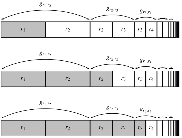
Figure 1: Stages 1, 2 and 3 of Algorithm B. Each row represents the output values of g0_r1,...,rk.After stage j the algorithm “knows” r1, . . . ,rj and can achieve perfect accuracy on the shaded

region.

Algorithm B works in a sequence of v stages. In stage j, the algorithm simply tries to obtain t0 independent example pairs for grj,rj+1and then uses Algorithm A.Assuming the algorithm succeeds

in each stage, after stage v algorithm B has obtained r1, . . . ,rv. It follows directly from the definition

of

G

0 that given r1, . . . ,rv, Algorithm B can construct a hypothesis that has error at most ₂v+32 (see

Figure 1) so we may take v=log1_ε+1 to obtain error at mostε.(Note that this implicitly assumes that log1_ε+1 is at most k; we deal with the case log1_ε+1>k at the end of the proof.)

If the learner fails to obtain r1, . . . ,rv, then either:

1. Independence was not achieved between every pair of examples;

2. Algorithm B fails to acquire t0pairs of examples for grj,rj+1 in some stage j; or

3. Algorithm B acquires t0 pairs of examples for grj,rj+1 but Algorithm A fails to obtain rj in

some stage j.

We choose the total number of examples so that each of these probabilities is bounded byδ/3 to achieve an overall failure probability of at mostδ.

many consecutive examples from the Updating Random Walk oracle. With this choice of s,the same argument as in the proof of Lemma 7 shows that the total failure probability for independence is at most δ₃.

We bound (2) assuming full independence between all pairs of examples. In stage j, Algorithm

B uses 4_·2jt0 pairs of examples. Observe that each pair of examples has both examples from

grj,rj+1 with probability at least 2−

(j+1)_{. By a Chernoff bound, the probability that less than t}0_{of the}

example pairs in stage j are from grj,rj+1 is at most e−

t0

8. Thus the overall probability of failure from

condition (2) is at most ve−t80 which is at mostδ/3 for t0≥ln(3v/δ).

We bound (3) assuming full independence between all pairs of examples as well. In stage j,we know by Fact 10 that after seeing t0=O(nk log(3vk/δ))pairs of examples for grj,rj+1, the probability

of failing to obtain rjis at mostδ/3v.Hence the overall failure probability from condition (3) is at

most δ₃.

We thus may take t0 =O(nk log(3vk/δ)) and achieve an overall failure probability of δ for obtaining r1, . . . ,rv. It follows that the overall number of examples required from the Updating

Random Walk oracle is poly(2v,n,log1_δ) =poly(n,1

ε,log1δ), which is what we required.

Finally, we observe that if log1_ε+1>k, since k=n

2−O(log n)a poly( 1

ε)-time algorithm may

run for, say, 22ntime steps and thus build an explicit truth table for the function. Such a table can be used to exactly identify each seed r1, . . . ,rkand output an exact representation of the target concept.

Acknowledgments

We warmly thank Tal Malkin for helpful discussions and the anonymous referees for useful sugges-tions that improved the presentation and readability of the paper.

References

D. Aldous and U. Vazirani. A Markovian extension of Valiant’s learning model. In Proceedings of

the Thirty-First Symposium on Foundations of Computer Science, pages 392–396, 1990.

P. Bartlett, P. Fischer, and K.U. H ¨offgen. Exploiting random walks for learning. Information and

Computation, 176(2):121–135, 2002.

A. Blum. Learning a function of r relevant variables (open problem). In Proc. 16th Annual COLT, pages 731–733, 2003.

A. Blum, M. Furst, J. Jackson, M. Kearns, Y. Mansour, and S. Rudich. Weakly learning DNF and characterizing statistical query learning using Fourier analysis. In Proceedings of the

Twenty-Sixth Annual Symposium on Theory of Computing, pages 253–262, 1994.

N. Bshouty, J. Jackson, and C. Tamon. More efficient PAC learning of DNF with membership queries under the uniform distribution. In Proceedings of the Twelfth Annual Conference on

Computational Learning Theory, pages 286–295, 1999.

N. Bshouty, E. Mossel, R. O’Donnell, and R. Servedio. Learning DNF from Random Walks. In

Proceedings of the 44th IEEE Symposium on Foundations on Computer Science, pages 189–198,

2003.

D. Gamarnik. Extension of the PAC framework to finite and countable Markov chains. In

Pro-ceedings of the 12th Annual Conference on Computational Learning Theory, pages 308–317,

1999.

O. Goldreich. Foundations of Cryptography: Volume 1, Basic Tools. Cambridge University Press, New York, 2001.

O. Goldreich, S. Goldwasser, and S. Micali. How to construct random functions. Journal of the

Association for Computing Machinery, 33(4):792–807, 1986.

J. H˚astad, R. Impagliazzo, L. Levin, and M. Luby. A pseudorandom generator from any one-way function. SIAM Journal on Computing, 28(4):1364–1396, 1999.

J. Jackson. An efficient membership-query algorithm for learning DNF with respect to the uniform distribution. Journal of Computer and System Sciences, 55:414–440, 1997.

J. Jackson, A. Klivans, and R. Servedio. Learnability beyond AC0. In Proceedings of the 34th ACM

Symposium on Theory of Computing, pages 776–784, 2002.

M. Kharitonov. Cryptographic hardness of distribution-specific learning. In Proceedings of the

Twenty-Fifth Annual Symposium on Theory of Computing, pages 372–381, 1993.

N. Linial, Y. Mansour, and N. Nisan. Constant depth circuits, Fourier transform and learnability.

Journal of the ACM, 40(3):607–620, 1993.

S. Roch. On learning thresholds of parities and unions of rectangles in random walk models.

Ran-dom Structures and Algorithms, 2006.

L. Valiant. A theory of the learnable. Communications of the ACM, 27(11):1134–1142, 1984.

K. Verbeurgt. Learning DNF under the uniform distribution in quasi-polynomial time. In