An Efficient Greedy Method for Unsupervised Feature Selection
Ahmed K. Farahat Ali Ghodsi Mohamed S. Kamel
University of Waterloo Waterloo, Ontario, Canada N2L 3G1 Email:{afarahat, aghodsib, mkamel}@uwaterloo.ca
Abstract—In data mining applications, data instances are typically described by a huge number of features. Most of these features are irrelevant or redundant, which negatively affects the efficiency and effectiveness of different learning algorithms. The selection of relevant features is a crucial task which can be used to allow a better understanding of data or improve the performance of other learning tasks. Although the selection of relevant features has been extensively studied in supervised learning, feature selection with the absence of class labels is still a challenging task. This paper proposes a novel method for unsupervised feature selection, which efficiently selects features in a greedy manner. The paper first defines an effective criterion for unsupervised feature selection which measures the reconstruction error of the data matrix based on the selected subset of features. The paper then presents a novel algorithm for greedily minimizing the reconstruction error based on the features selected so far. The greedy algorithm is based on an efficient recursive formula for calculating the reconstruction error. Experiments on real data sets demonstrate the effectiveness of the proposed algorithm in comparison to the state-of-the-art methods for unsupervised feature selection.
Keywords-Feature Selection; Greedy Algorithms; Unsuper-vised Learning
I. INTRODUCTION
Data instances are typically described by a huge number of features. Most of these features are either redundant, or irrelevant to the data mining task at hand. Having a large number of redundant and irrelevant features negatively affects the performance of the underlying learning algo-rithms, and makes them more computationally demanding. Therefore, reducing the dimensionality of the data is a fundamental task for machine learning and data mining applications.
Throughout past years, two approaches have been pro-posed for dimension reduction; feature selection, and fea-ture extraction. Feafea-ture selection (also known as variable selection or subset selection) searches for a relevant subset of existing features, while feature extraction (also known as feature transformation) learns a new set of features which combines existing features. These methods have been employed with both supervised and unsupervised learning, where in the case of supervised learning class labels are used to guide the selection or extraction of features.
Feature extraction methods produce a set of continuous vectors which represent data instances in the space of the
extracted features. Accordingly, most of these methods ob-tain unique solutions in polynomial time, which make these methods more attractive in terms of computational complex-ity. On the other hand, feature selection is a combinatorial optimization problem which is NP-hard, and most feature selection methods depend on heuristics to obtain a subset of relevant features in a manageable time. Nevertheless, feature extraction methods usually produce features which are difficult to interpret, and accordingly feature selection is more appealing in applications where understanding the meaning of features is crucial for data analysis.
Feature selection methods can be categorized into wrapper and filter methods. Wrapper methods wrap feature selection around the learning process and search for features which enhance the performance of the learning task. Filter methods, on the other hand, analyze the intrinsic properties of the data, and select highly-ranked features according to some criterion before doing the learning task. Wrapper methods are computationally more complex than filter methods as they depend on deploying the learning models many times until a subset of relevant features are found.
This paper presents an effective filter method for un-supervised feature selection. The method is based on a novel criterion for feature selection which measures the reconstruction error of the data matrix based on the subset of selected features. The paper presents a novel recursive formula for calculating the criterion function as well as an efficient greedy algorithm to select features. The greedy algorithm selects at each iteration the most representative feature among the remaining features, and then eliminates the effect of the selected features from the data matrix. This step makes it less likely for the algorithm to select fea-tures that are similar to previously selected feafea-tures, which accordingly reduces the redundancy between the selected features. In addition, the use of the recursive criterion makes the algorithm computationally feasible and memory efficient compared to the state of the art methods for unsupervised feature selection.
The rest of this paper is organized as follows. Section II defines the notations used throughout the paper. Section III discusses previous work on filter methods for unsupervised feature selection. Section IV presents the proposed feature selection criterion. Section V presents a novel recursive for-mula for the feature selection criterion. Section VI proposes
an effective greedy algorithm for feature selection as well as memory and time efficient variants of the algorithm. Section VII presents an empirical evaluation of the proposed method. Finally, Section VIII concludes the paper.
II. NOTATIONS
Throughout the paper, scalars, vectors, sets, and matrices are shown in small, small bold italic, script, and capital letters, respectively. In addition, the following notations are used.
For a vectorx∈Rp:
xi i-th element ofx.
kxk the Euclidean norm (`2-norm) ofx.
For a matrixA∈Rp×q:
Aij (i, j)-th entry ofA. Ai: i-th row ofA.
A:j j-th column of A.
AS: the sub-matrix ofAwhich consists of the set
S of rows.
A:S the sub-matrix ofAwhich consists of the set S of columns.
˜
A a low rank approximation ofA.
˜
AS a rank-kapproximation ofAbased on the set S of columns, where|S|=k.
kAkF the Frobenius norm ofA:kAkF = Σi,jA2ij III. PREVIOUSWORK
Many filter methods for unsupervised feature selection depend on the Principal Component Analysis (PCA) method [1] to search for the most representative features. PCA is the best-known method for unsupervised feature extraction which finds directions with maximum variance in the feature space (namely principal components). The principal compo-nents are also those directions that achieve the minimum reconstruction error for the data matrix. Jolliffe [1] suggests different algorithms to use PCA for unsupervised feature selection. In these algorithms, features are first associated with principal components based on the absolute value of their coefficients, and then features corresponding to the first (or last) principal components are selected (or deleted). This can be done once or recursively (i.e., by first selecting or deleting some features and then recomputing the principal components based on the remaining features). Similarly, sparse PCA [2], a variant of PCA which produces sparse principal components, can also be used for feature selection. This can be done by selecting for each principal component the subset of features with non-zero coefficients. However, Masaeli et al. [3] showed that these sparse coefficients may be distributed across different features and accordingly are not always useful for feature selection. Another iterative ap-proach is suggested by Cui and Dy [4], in which the feature that is most correlated with the first principal component is selected, and then other features are projected onto the direction orthogonal to that feature. These steps are repeated until the required number of features are selected. Lu et al.
[5] suggests a different PCA-based approach which applies k-means clustering to the principal components, and then selects the features that are close to clusters’ centroids. Boutsidis et al. [6], [7] propose a feature selection method that randomly samples features based on probabilities calcu-lated using the k-leading singular values of the data matrix. In [6], random sampling is used to reduce the number of candidate features, and then the required number of features is selected by applying a complex subset selection algorithm on the reduced matrix. In [7], the authors derive a theoretical guarantee for the error of the k-means clustering when features are selected using random sampling. However, the-oretical guarantees for other clustering algorithms were not explored in this work. Recently, Masaeli et al. [3] propose an algorithm called Convex Principal Feature Selection (CPFS). CPFS formulates feature selection as a convex continuous optimization problem which minimizes the mean-squared-reconstruction error of the data matrix (a PCA-like criterion) with sparsity constraints. This is a quadratic programming problem with linear constraints, which was solved using a projected quasi-Newton method.
Another category of unsupervised feature selection meth-ods are based on selecting features that preserve similarities between data instances. Most of these methods first construct a k nearest neighbor graph between data instances, and then select features that preserve the structure of that graph. Examples for these methods include the Laplacian score (LS) [8] and the spectral feature selection method (a.k.a., SPEC) [9]. The Laplacian score (LS) [8] calculates a score for each feature based on the graph Laplacian and degree matrices. This score quantifies how each feature preserves similarity between data instances and their neighbors in the graph. Spectral feature selection [9] extends this idea and presents a general framework for ranking features on a k nearest neighbor graph.
Some methods directly select features which preserve the cluster structure of the data. The Q−α algorithm [10] measures the goodness of a subset of features based on the clustering quality (namely cluster coherence) when data is represented using only those features. The authors define a feature weight vector, and propose an iterative algorithm that alternates between calculating the cluster coherence based on current weight vector and estimating a new weight vector that maximizes that coherence. This algorithm converges to a local minimum of the cluster coherence and produces a sparse weight vector that indicates which features should be selected. Recently, Cai et al. [11] propose an algorithm called Multi-Cluster Feature Selection (MCFS) which selects a subset of features such that the multi-cluster structure of the data is preserved. To achieve that, the authors em-ploy a method similar to spectral clustering [12], which first constructs a k nearest neighbor graph over the data instances, and then solves a generalized eigenproblem over the graph Laplacian and degree matrices. After that, for each
eigenvector, anL1-regularized regression problem is solved to represent each eigenvector using a sparse combination of features. Features are then assigned scores based on these coefficients and highly scored features are selected. The authors show experimentally that the MCFS algorithm outperforms Laplacian score (SC) and theQ−αalgorithm. Another well-known approach for unsupervised feature selection is the Feature Selection using Feature Similarity (FSFS) method suggested by Mitra et al. [13]. The FSFS method groups features into clusters and then selects a representative feature for each cluster. To group features, the algorithm starts by calculating pairwise similarities between features, and then it constructs a k nearest neighbor graph over the features. The algorithm then selects the feature with the most compact neighborhood and removes all its neighbors. This process is repeated on the remaining fea-tures until all feafea-tures are either selected or removed. The authors also suggested a new feature similarity measure, namely maximal information compression, which quantifies the minimum amount of information loss when one feature is represented by the other.
In comparison to previous work, the greedy feature selec-tion method proposed in this paper uses a PCA-like criterion which minimizes the reconstruction error of the data matrix based on the selected subset of features. In contrast to traditional PCA-based methods, the proposed algorithm does not calculate the principal components, which is computa-tionally demanding. Unlike Laplacian score (LS) [8] and its extension [9], the greedy feature selection method does not depend on calculating pairwise similarity between instances. It also does not calculate eigenvalue decomposition over the similarity matrix as the Q −α algorithm [10] and Multi-Cluster Feature Selection (MCFS) [11] do. The feature selection criterion presented in this paper is similar to that of Convex Principal Feature Selection (CPFS) [3] as both minimize the reconstruction error of the data matrix. While the method presented here uses a greedy algorithm to minimize a discrete optimization problem, CPFS solves a quadratic programming problem with sparsity constraints. In addition, the number of features selected by the CPFS depends on a regularization parameter λ which is difficult to tune. Similar to the method proposed by Cui and Dy [4], the method presented in this paper removes the effect of each selected feature by projecting other features to the direction orthogonal to that selected feature. However, the method proposed by Cui and Dy is computationally very complex as it requires the calculation of the first princi-pal component for the whole matrix after each iteration. The Feature Selection using Feature Similarity (FSFS) [13] method employs a similar greedy approach which selects the most representative feature, and then eliminates its neighbors in the feature similarity graph. The FSFS method, however, depends on a computationally complex measure for calculating similarity between features. As shown in
Section VII, experiments on real data sets show that the proposed algorithm outperforms the Feature Selection using Feature Similarity (FSFS) method [13], Laplacian score (SC) [8], and Multi-Cluster Feature Selection (MCFS) [11] when applied with different clustering algorithms.
IV. FEATURESELECTIONCRITERION
This section defines a novel criterion for unsupervised feature selection. The criterion measures the reconstruction error of data matrix based on the selected subset of features. The goal of the proposed feature selection algorithm is to select a subset of features that minimizes this reconstruction error.
Definition 1: (Unsupervised Feature Selection Crite-rion)LetAbe anm×ndata matrix whose rows represent the set of data instances and whose columns represent the set of features. The feature selection criterion is defined as:
F(S) =kA−P(S)Ak2F
whereS is the set of the indices of selected features, and P(S) is an m×m projection matrix which projects the columns ofAonto the span of the setS of columns.
The criterion F(S)represents the sum of squared errors between original data matrixAand its rank-kapproximation based on the selected set of features (wherek=|S|):
˜
AS =P(S)A. (1)
The projection matrix P(S) can be calculated as: P(S)=A:S AT:SA:S
−1
AT:S (2)
where A:S is the sub-matrix of A which consists of the columns corresponding to S. It should be noted that if the subset of featuresS is known, the projection matrixP(S)is
the closed-form solution of the least-squares problem which minimizes F(S).
The goal of the feature selection algorithm presented in this paper is to select a subsetSof features such thatF(S)
is minimized.
Problem 1: (Unsupervised Feature Selection) Find a subset of featuresL such that,
L=arg min S
F(S).
This is an NP-hard combinatorial optimization problem. In Section V, a recursive formula for the selection criterion is presented. This formula allows the development of an efficient algorithm to greedily minimize F(S). The greedy algorithm is presented in Section VI.
V. RECURSIVESELECTIONCRITERION
In this section, a recursive formula is derived for the feature selection criterion presented in Section IV. This formula is based on a recursive formula for the projection matrix P(S) which can be derived as follows.
Lemma 1: Given a set of featuresS. For any P ⊂ S, P(S)=P(P)+R(R)
where R(R) is a projection matrix which projects the
columns of E = A−P(P)A onto the span of the subset
R=S \ P of columns:
R(R)=E:R ET:RE:R −1
E:TR. Proof: Define a matrixB =AT
:SA:S which represents the inner-product over the columns of the sub-matrix A:S. The projection matrix P(S) can be written as:
P(S)=A:SB−1AT:S (3) Without loss of generality, the columns and rows ofA:S andB in Eq. (3) can be rearranged such that the first sets of rows and columns correspond toP:
A:S = A:P A:R , B = BPP BPR BT PR BRR where BPP = AT:PA:P, BPR = AT:PA:R and BRR = AT:RA:R.
LetBRR−BPRT BPP−1BPRbe the Schur complement [14] ofBPP inB. Use the block-wise inversion formula [14] of B−1 and substitute withA
:S andB−1 in Eq. (3): P(S)= A:P A:R BPP−1 +BPP−1BPRS−1BPRT B −1 PP −B −1 PPBPRS−1 −S−1BT PRB− 1 PP S−1 AT :P AT:R
The right-hand side can be simplified to: P(S)=A:PBPP−1A T :P + A:R−A:PBPP−1BPRS−1 AT:R−B T PRB −1 PPA T :P (4) The first term of Eq. (4) is the projection matrix which projects the columns of A onto the span of the subset P of columns:P(P)=A
:PBPP−1AT:P. The second term can be simplified as follows. Let E be an m×n residual matrix which is calculated as: E =A−P(P)A. It can be shown thatE:R=A:R−A:PBPP−1BPR, andS=E:TRE:R. Hence, the second term of Eq. (4) is the projection matrix which projects the columns ofE onto the span of the subsetRof columns:
R(R)=E:R ET:RE:R −1
E:TR. (5) This proves that P(S) can be written in terms ofP(P) and
R as:P(S)=P(P)+R(R)
This means that projection matrixP(S)can be constructed
in a recursive manner by first calculating the projection matrix which projects the columns of A onto the span of the subsetP of columns, and then calculating the projection matrix which projects the columns of the residual matrix
onto the span of the remaining columns. Based on this lemma, a recursive formula can be developed forA˜S.
Corollary 1: Given a matrixA and a subset of columns S. For anyP ⊂ S,
˜
AS = ˜AP + ˜ER
where E =A−P(P)A, and E˜R is the low-rank approxi-mation of E based on the subset R=S \ P of columns.
Proof:Using Lemma (1), and substituting withP(S)in Eq. (1) gives:
˜
AS =P(P)A+E:R E:TRE:R −1
E:TRA (6) The first term is the low-rank approximation of A based on P: AP˜ = P(P)A. The second term is equal to ER˜ as ET:RA = E:TRE. To prove that, multiplying E:TR by E =
A−P(P)A gives:
E:TRE=E:TRA−E:TRP(P)A.
UsingE:R=A:R−P(P)A:R, the expressionE:TRP(P)can be written as:
E:TRP(P)=AT:RP(P)−AT:RP(P)P(P).
This is equal to 0 as P(P)P(P) = P(P) (A property of
projection matrices). This means that ET
:RA=ET:RE. Sub-stituting ET
:RA withE:TRE in Eq. (6) proves the corollary. Based on Corollary (1), a recursive formula for the feature selection criterion can be developed as follows.
Theorem 2: Given a set of featuresS. For any P ⊂ S, F(S) =F(P)− kER˜ k2
F
whereE =A−P(P)A, and E˜
R is the low-rank approxi-mation ofE based on the subset R=S \ P of columns.
Proof: Substituting withP(S)in Eq. (1) gives:
F(S) =kA−AS˜ kF2 =kA−AP˜ −ER˜ k
2
F =kE−ER˜ k
2
F
Using the relation between the Frobenius norm and the trace function1, the right-hand side can be expressed as:
kE−ER˜ k2 F =trace E−E˜(R) T E−ER˜ =trace(ETE−2ETE˜R+ ˜ERTE˜R) AsR(R)R(R)=R(R), the expressionE˜T RE˜Rcan be written as: ˜ ERTE˜R=ETR(R)R(R)E=ETR(R)E=ETE˜R This means that: F(S) = kE−ER˜ k2
F = trace(E TE− ˜ ERE˜R) =kEk2F − kE˜Rk 2 F. Replacing kEk 2 F with F(P) proves the theorem.
The termkE˜Rk2F represents the decrease in reconstruction error achieved by adding the subsetRof features to P. In
1kAk2
the following section, a novel greedy heuristic is presented to optimize the feature selection criterion based on this recursive formula.
VI. GREEDYSELECTIONALGORITHM
This section presents an efficient greedy algorithm to optimize the feature selection criterion presented in Section IV. The algorithm selects at each iteration one feature such that the reconstruction error for the new set of features is minimum. This problem can be formulated as follows.
Problem 2: (Greedy Feature Selection) At iteration t, find featurel such that,
l=arg min i
F(S ∪ {i}) (7) whereS is the set of features selected during the firstt−1
iterations.
A na¨ıve implementation of the greedy algorithm is to calculate the reconstruction error for each candidate feature, and then select the feature with the smallest error. This implementation is however computationally very complex as it requiresO(m2n2)floating-point operations per iteration.
A more efficient approach is to use the recursive formula for calculating the reconstruction error. Using Theorem 2,
F(S ∪ {i}) =F(S)− kE˜{i}k2F,
where E = A −A˜S. Since F(S) is a constant for all candidate features, an equivalent criterion is:
l=arg max i
kE˜{i}k2F (8) This formulation selects the feature l which achieves the maximum decrease in reconstruction error. The new objec-tive function ˜ E{i} 2
F can be simplified as follows:
˜ E{i} 2 F
=traceE˜{i}T E˜{i}=traceETR({i})E
=traceETE:i E:TiE:i −1 E:TiE = 1 ET :iE:i trace ETE:iE:TiE = ETE:i 2 ET :iE:i . This defines the following simplified problem.
Problem 3: (Simplified Greedy Feature Selection) At iterationt, find feature l such that,
l=arg max i ETE:i 2 ET :iE:i (9) where E =A−A˜S, and S is the set of features selected during the firstt−1 iterations.
The computational complexity of this selection criterion isO n2m
per iteration, and it requiresO(nm)memory to store the residual of the whole matrix,E, after each iteration. In the rest of this section, two novel techniques are proposed to reduce the memory and time requirements of this selection criterion.
A. Memory-Efficient Criterion
This section proposes a memory-efficient algorithm to calculate the simplified feature selection criterion without explicitly calculating and storing the residual matrix E at each iteration. The algorithm is based on a recursive formula for calculating the residual matrixE.
LetS(t)denote the set of features selected during the first
t−1 iterations, E(t) denote the residual matrix at the start
of thet-th iteration (i.e.,E(t)=A−A˜
S(t)), andl(t) be the feature selected at iterationt. The following lemma gives a recursive formula for residual matrix at the end of iteration t,E(t+1).
Lemma 2: E(t+1)can be calculated recursively as:
E(t+1)= (E−E:lE T :l ET :lE:l E)(t).
Proof: Using Corollary 1, A˜S∪{l} = A˜S + ˜E{l}. Subtracting both sides fromA, and substitutingA−A˜S∪{l} andA−A˜S withE(t+1) andE(t)respectively gives:
E(t+1)= (E−E˜{l})(t)
Using Eqs (1) and (2), E˜{l} can be expressed as E:l(E:TlE:l)−1E:Tl
E. SubstitutingE˜{l} with this formula in the above equation proves the lemma.
Let G be an n×n which represents the inner-products over the columns of the residual matrixE:G=ETE. The following corollary is a direct result of Lemma 2.
Corollary 3: G(t+1) can be calculated recursively as:
G(t+1)= (G−G:lG T
:l Gll )
(t).
Proof:This corollary can be proved by substituting with E(t+1)T (Lemma 2) in G(t+1) = E(t+1)TE(t+1), and
us-ing the fact that E:l(E:TlE:l)−1ET:l
E:l(E:TlE:l)−1E:Tl
=
E:l(E:TlE:l)−1ET:l.
To simplify the derivation of the memory-efficient algo-rithm, at iteration t, define δ=G:l andω =G:l/
√ Gll= δ/√δl. This means thatG(t+1) can be calculated in terms ofG(t) andω(t) as follows:
G(t+1)= (G−ωωT)(t), (10) or in terms ofA and previousω’s as:
G(t+1)=ATA− t
X
r=1
(ωωT)(r). (11)
δ(t)andω(t)can be calculated in terms ofAand previous
ω’s as follows: δ(t)=ATA:l− t−1 X r=1 ω(lr)ω(r), ω(t)=δ(t)/ q δ(lt).
The simplified feature selection criterion can be expressed in terms ofGas: l=arg max i kG:ik 2 Gii
The following theorem gives recursive formulas for cal-culating the simplified feature selection criterion without explicitly calculatingE nor G.
Theorem 4: Letfi=kG:ik
2
andgi=Giibe the numer-ator and denominnumer-ator of the simplified criterion function for a featurei respectively, f = [fi]i=1..n, and g= [gi]i=1..n. Then, f(t)=f −2ω◦ATAω−Σt−r=12ω(r)Tωω(r) +kωk2(ω◦ω)(t−1), g(t)=g−(ω◦ω) (t−1) .
where◦represents the Hadamard product operator. Proof:Based on Eq. (10), f(it) can be calculated as:
f(it)=kG:ik2 (t) = kG:i−ωiωk2 (t−1) = (G:i−ωiω)T(G:i−ωiω) (t−1) = GT:iG:i−2ωiGT:iω+ω 2 ikωk 2(t−1) = fi−2ωiGT:iω+ω 2 ikωk 2(t−1) . (12)
Similarly, g(it)can be calculated as:
g(it)=Gii(t)= Gii−ω2i(t−1) = gi−ω2i(t−1) . (13) Let f = [fi]i=1..nand g = [gi]i=1..n,f (t) and g(t) can be expressed as: f(t)= f−2 (ω◦Gω) +kωk2(ω◦ω)(t−1) , g(t)= (g−(ω◦ω))(t−1), (14)
where◦represents the Hadamard product operator, andk.k is the `2 norm.
Based on the recursive formula of G (Eq. 11), the term Gωat iteration(t−1)can be expressed as:
Gω=ATA−Σt−r=12 ωωT(r)ω =ATAω−Σrt−=12ω(r)Tωω(r)
(15)
Substitute with Gω in Equation (14) gives the update formulas forf andg
This means that the greedy criterion can be memory-efficient by only maintaining two score variables for each feature,fiandgi, and updating them at each iteration based on their previous values and the selected features so far.
B. Partition-Based Criterion
The simplified feature selection criterion calculates, at each iteration, the inner-products between each candidate feature E:i and other features E. The computational com-plexity of these inner-products isO(nm)per candidate fea-ture (orO(n2m)per iteration). When the memory-efficient
update formulas are used, the computational complexity is reduced toO(nm)per iteration (that of calculatingATAω). However, the complexity of calculating the intial value off
is stillO(n2m).
In order to reduce this computational complexity, a novel partition-based criterion is proposed, which reduces the number of inner products to be calculated at each iteration. The criterion partitions features intocnrandom groups, and selects the feature which best represents the centroids of these groups. LetPj be the set of feature that belong to the j-th partition,P={P1,P2, ...Pc}be a random partitioning of features intoc groups, andB be anm×c matrix whose elementj-th column is the sum of feature vectors that belong to the j-th group: B:j = Pr∈PjA:r. The use of the sum function (instead of mean) weights each column of B with the size of the corresponding group. This avoids any bias towards larger groups when calculating the sum of inner-products.
The simplified selection criterion can be written as: Problem 4: (Simplified Partition-Based Greedy Fea-ture Selection) At iterationt, find feature l such that,
l=arg max i FTE:i 2 ET :iE:i (16)
where E = A−A˜S, S is the set of features selected during the first t−1 iterations, F:j = Pr∈PjE:r, and P = {P1,P2, ...Pc} is a random partitioning of features into c groups.
Similar to E (Lemma 2), F can be calculated in a recursive manner as follows:
F(t+1)= (F−E:lE T
:l E:TlE:l
F)(t).
This means that random partitioning can be done once at the start of the algorithm. After that, F is initialized to B and then updated recursively using the above formula. The computational complexity of calculating B is O(nm)
if the data matrix is full. However, this complexity could be considerably reduced if the data matrix is very sparse.
Further, a memory-efficient variant of the partition-based algorithm can be developed as follows. LetH be anc×n matrix whose elementHji is the inner-product of the cen-troid of thej-th group and the i-th feature, weighted with the size of thej-th group:H =FTE. Similarly, H can be calculated recursively as follows:
H(t+1)= (H−H:lG T
:l Gll )
Defineγ =H:l andυ =H:l/
√
Gll=γ/√δl. H(t+1) can be calculated in terms ofH(t),υ(t) andω(t) as follows:
H(t+1)= (H−υωT)(t), (17) or in terms of Aand previousω’s andυ’s as:
H(t+1)=BTA− t
X
r=1
(υωT)(r). (18)
γ(t)andυ(t)can be calculated in terms ofA,Band previous ω’s andυ’s as follows: γ(t)=BTA:l− t−1 X r=1 ω(lr)υ(r), υ(t)=γ(t)/ q δ(lt).
The simplified partition-based selection criterion can be expressed in terms ofH andGas:
l=arg max i
kH:ik
2
Gii
Similar to Theorem 4, the following theorem derives re-cursive formulas for the simplified partition-based criterion function.
Theorem 5: Let fi = kH:ik2 and gi = Gii be the numerator and denominator of the partition-based simplified criterion function for a featureirespectively,f = [fi]i=1..n, andg= [gi]i=1..n. Then, f(t)=f−2ω◦ATBυ−Σt−r=12υ(r)Tυω(r) +kυk2(ω◦ω)(t−1), g(t)=g−(ω◦ω) (t−1) .
where◦represents the Hadamard product operator. Proof: The proof is similar to that of Theorem 4. It can be easily derived by using the recursive formula forH:i instead of that for G:i.
In these update formulas, ATB can be calculated once and then used in different iterations. This makes the compu-tational complexity of the new update formulas isO(nc)per iteration. Algorithm 1 shows the complete greedy algorithm. The computational complexity of the algorithm is dominated by that of calculating ATA
:l in Step (b) which is of O(mn) per iteration. The other complex step is that of calculating the initialf, which isO(mnc). However, these steps can be implemented in an efficient way if the data matrix is sparse. The total complexity of the algorithm is O(max(mnk, mnc)), wherekis the number of features and c is the number of random partitions.
Algorithm 1Greedy Feature Selection Inputs:Data matrix A, Number of features k
Outputs:Selected featuresS, Steps:
1) InitializeS ={ }, Generate a random partitioningP, Calculate B:B:j=Pr∈PjA:r 2) Initializef(0)i =kBTA :ik2, andg (0) i =AT:iA:i 3) Repeat t= 1→k: a) l=arg max i fi(t)/gi(t), S=S ∪ {l} b) δ(t)=ATA :l−P t−1 r=1ω (r) l ω (r) c) γ(t)=BTA :l−P t−1 r=1ω (r) l υ (r) d) ω(t)=δ(t)/qδ(t) l ,υ (t)=γ(t)/qδ(t) l e) Updatefi’s,gi’s (Theorem 5)
VII. EXPERIMENTS ANDRESULTS
Experiments have been conducted on four benchmark data sets, whose properties are summarized in Table I. These data sets were recently used by Cai et al. [11] to evaluate different feature selection methods in comparison to the Multi-Cluster Feature Selection (MCFS) method2.
In this section, seven methods for unsupervised feature selection are compared3:
1) PCA-LRG: is a PCA-based method that selects fea-tures associated with the firstk principal components [1]. It has been shown that by Masaeli et al. [3] that this method achieves a low reconstruction error of the data matrix compared to other PCA-based methods4. 2) FSFS: is the Feature Selection using Feature
Sim-ilarity [13] method with the maximal information compression as the feature similarity measure. 3) LS: is the Laplacian Score (LS) [8] method.
4) SPEC: is the spectral feature selection method [9] using all the eigenvectors of the graph Laplacian. 5) MCFS: is the Multi-Cluster Feature Selection [11]
method which has been shown to outperform other methods that preserve the cluster struture of the data. 6) GreedyFS: The basic greedy algorithm presented in this paper (using recursive update formulas forf and
g but without random partitioning).
7) PartGreedyFS: The partition-based greedy algorithm (Algorithm 1).
2Data sets are available at:
http://www.zjucadcg.cn/dengcai/Data/FaceData.html http://www.zjucadcg.cn/dengcai/Data/MLData.html
3The following implementations were used:
FSFS: http://www.facweb.iitkgp.ernet.in/∼pabitra/paper/fsfs.tar.gz
LS: http://www.zjucadcg.cn/dengcai/Data/code/LaplacianScore.m SPEC: http://featureselection.asu.edu/algorithms/fs uns spec.zip MCFS: http://www.zjucadcg.cn/dengcai/Data/code/MCFS p.m
4The CPFA method was not included in the comparison as its imple-mentation details were not completely specified in [3].
Similar to previous work [8], [11], the feature selection methods were compared based on their performance in clustering tasks. Two clustering algorithms were used to compare different methods: the well-known k-means algo-rithm [15], and the state-of-the-art affinity propagation (AP) algorithm [16]. For each feature selection method, the k -means algorithm is applied to the rows of the data matrix whose columns are the subset of the selected features. For the affinity propagation, a distance matrix is first calculated based on the selected subset of features, and then the algorithm is applied to the negative of this distance matrix. The preference vector, which controls the number of clusters, is set to the median of each column of the similarity matrix, as suggested by Frey and Dueck [16]. After the clustering is performed using the subset of selected features, the cluster labels are compared to ground-truth labels provided by human annotators and the Normalized Mutual Information (NMI) [17] between clustering labels and the class labels is calculated. The clustering performance with all features is also calculated and used as a baseline. In addition to clustering performance, the run times of different feature selection methods are compared. This run time includes the time for selecting features only, and not the run time of the clustering algorithm.
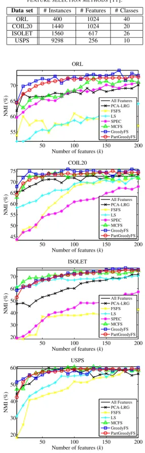
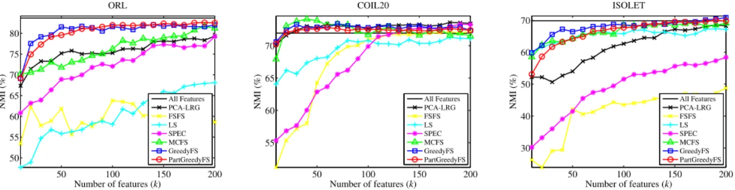
Figures 1 and 2 show the clustering performance for the k-means and affinity propagation (AP) algorithms respec-tively5. It can be observed from results that the greedy feature selection methods (GreedyFS and PartGreedyFS) outperforms thePCA-LRG,FSFS,LS, andSPECmethods for almost all data sets. TheGreedyFSmethod outperforms MCFSfor many data sets, while its partition-based variant, PartGreedyFS, outperformsMCFS for some data sets and shows comparable performance for others.
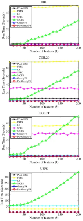
Figure 3 shows the run times of different feature selection methods. It can be observed that FSFSis computationally more expensive than other methods as it depends on cal-culating complex similarities between features. TheMCFS method, however efficient, is more computationally complex than Laplacian score (LS) and the proposed greedy methods. It can be also observed that for data sets with large number of instances (like USPS), theMCFSmethod, the Laplacian score (LS) and theSPECbecome very computationally de-manding as they depend on calculating pairwise similarities between instances. Figure 4 shows the run times of the PCA-LRG and Laplacian score (LS) methods in comparison to the proposed greedy methods. It can be observed that the complexity of the Laplacian score increases as the size of the data set increases. It can also be observed that the partition-based greedy feature selection (PartGreedyFS) is more efficient than the basic greedy feature selection (GreedyFS).
5The implementations of SPEC and AP do not scale to run on the USPS data set on the used simulation machine.
Table I
THE PROPERTIES OF DATA SETS USED TO EVALUATE DIFFERENT
FEATURE SELECTION METHODS[11].
Data set # Instances # Features # Classes
ORL 400 1024 40 COIL20 1440 1024 20 ISOLET 1560 617 26 USPS 9298 256 10 50 100 150 200 55 60 65 70 ORL Number of features (k) N M I (% ) All Features PCA-LRG FSFS LS SPEC MCFS GreedyFS PartGreedyFS 50 100 150 200 45 50 55 60 65 70 75 COIL20 Number of features (k) N M I (% ) All Features PCA-LRG FSFS LS SPEC MCFS GreedyFS PartGreedyFS 50 100 150 200 20 30 40 50 60 70 ISOLET Number of features (k) N M I (% ) All Features PCA-LRG FSFS LS SPEC MCFS GreedyFS PartGreedyFS 50 100 150 200 20 30 40 50 60 USPS Number of features (k) N M I (% ) All Features PCA-LRG FSFS LS MCFS GreedyFS PartGreedyFS
Figure 1. The k-means clustering performance of different feature selection methods.
50 100 150 200 50 55 60 65 70 75 80 ORL Number of features (k) N M I (% ) All Features PCA-LRG FSFS LS SPEC MCFS GreedyFS PartGreedyFS 50 100 150 200 55 60 65 70 COIL20 Number of features (k) N M I (% ) All Features PCA-LRG FSFS LS SPEC MCFS GreedyFS PartGreedyFS 50 100 150 200 30 40 50 60 70 ISOLET Number of features (k) N M I (% ) All Features PCA-LRG FSFS LS SPEC MCFS GreedyFS PartGreedyFS
Figure 2. The affinity propagation (AP) clustering performance of different feature selection methods.
VIII. CONCLUSIONS
This paper presents a novel greedy algorithm for unsuper-vised feature selection. The algorithm optimizes a feature selection criterion which measures the reconstruction error of the data matrix based on the subset of selected features. The paper proposes a novel recursive formula for calculating the feature selection criterion, which is then employed to develop an efficient greedy algorithm for feature selection. In addition, two memory and time efficient variants of the feature selection algorithm are proposed. It has been empirically shown that the proposed algorithm achieves better clustering performance compared to state-of-the-art methods for feature selection, and is less computationally demanding than methods that give comparable clustering performance.
REFERENCES
[1] I. Jolliffe,Principal Component Analysis, 2nd ed. Springer, 2002.
[2] H. Zou, T. Hastie, and R. Tibshirani, “Sparse principal component analysis,”J. Comput. Graph. Stat., vol. 15, no. 2, pp. 265–286, 2006.
[3] M. Masaeli, Y. Yan, Y. Cui, G. Fung, and J. Dy, “Convex prin-cipal feature selection,” inProceedings of SIAM International Conference on Data Mining (SDM), 2010, pp. 619–628. [4] Y. Cui and J. Dy, “Orthogonal principal feature selection,” in
the Sparse Optimization and Variable Selection Workshop at the International Conference on Machine Learning (ICML), 2008.
[5] Y. Lu, I. Cohen, X. Zhou, and Q. Tian, “Feature selection using principal feature analysis,” inProceedings of the 15th International Conference on Multimedia. New York, NY, USA: ACM, 2007, pp. 301–304.
[6] C. Boutsidis, M. W. Mahoney, and P. Drineas, “Unsupervised feature selection for principal components analysis,” in Pro-ceeding of the 14th ACM SIGKDD International Conference
on Knowledge Discovery and Data Mining (KDD’08). New
York, NY, USA: ACM, 2008, pp. 61–69.
[7] C. Boutsidis, M. Mahoney, and P. Drineas, “Unsupervised feature selection for the k-means clustering problem,” in Advances in Neural Information Processing Systems 22, Y. Bengio, D. Schuurmans, J. Lafferty, C. K. I. Williams, and A. Culotta, Eds., 2009, pp. 153–161.
[8] X. He, D. Cai, and P. Niyogi, “Laplacian score for feature selection,” in Advances in Neural Information Processing Systems 18, Y. Weiss, B. Sch¨olkopf, and J. Platt, Eds. Cam-bridge, MA, USA: MIT Press, 2006, pp. 507–514.
[9] Z. Zhao and H. Liu, “Spectral feature selection for supervised and unsupervised learning,” inProceedings of the 24th Inter-national Conference on Machine learning. New York, NY, USA: ACM, 2007, pp. 1151–1157.
[10] L. Wolf and A. Shashua, “Feature selection for unsupervised and supervised inference: The emergence of sparsity in a weight-based approach,” J. Mach. Learn. Res., vol. 6, pp. 1855–1887, 2005.
[11] D. Cai, C. Zhang, and X. He, “Unsupervised feature selection for multi-cluster data,” in Proceedings of the 16th ACM SIGKDD International Conference on Knowledge Discovery
and Data Mining (KDD’10). New York, NY, USA: ACM,
2010, pp. 333–342.
[12] A. Ng, M. Jordan, and Y. Weiss, “On spectral clustering: Analysis and an algorithm,” inAdvances in Neural
Informa-tion Processing Systems 14 (NIPS’01). Cambridge, MA,
USA: MIT Press, 2001, pp. 849–856.
[13] P. Mitra, C. Murthy, and S. Pal, “Unsupervised feature se-lection using feature similarity,” IEEE Trans. Pattern Anal. Mach. Intell., vol. 24, no. 3, pp. 301–312, 2002.
[14] H. L¨utkepohl,Handbook of Matrices. John Wiley & Sons Inc, 1996.
[15] A. Jain and R. Dubes, Algorithms for Clustering Data. Prentice-Hall, Inc., 1988.
[16] B. Frey and D. Dueck, “Clustering by passing messages between data points,” Science, vol. 315, no. 5814, p. 972, 2007.
[17] A. Strehl and J. Ghosh, “Cluster ensembles—a knowledge reuse framework for combining multiple partitions,”J. Mach. Learn. Res., vol. 3, pp. 583–617, 2003.
50 100 150 200 10 20 30 40 ORL Number of features (k) Ru n T im e (S ec o n d s) PCA-LRG FSFS LS SPEC MCFS GreedyFS PartGreedyFS 50 100 150 200 20 40 60 80 COIL20 Number of features (k) Ru n T im e (S ec o n d s) PCA-LRG FSFS LS SPEC MCFS GreedyFS PartGreedyFS 50 100 150 200 10 20 30 40 ISOLET Number of features (k) Ru n T im e (S ec o n d s) PCA-LRG FSFS LS SPEC MCFS GreedyFS PartGreedyFS 50 100 150 200 50 100 150 200 250 300 USPS Number of features (k) Ru n T im e (S ec o n d s) PCA-LRG FSFS LS MCFS GreedyFS PartGreedyFS
Figure 3. The run times of different feature selection methods.
50 100 150 200 0.5 1 1.5 2 2.5 ORL Number of features (k) Ru n T im e (S ec o n d s) PCA-LRG LS GreedyFS PartGreedyFS 50 100 150 200 1 2 3 4 5 6 7 COIL20 Number of features (k) Ru n T im e (S ec o n d s) PCA-LRG LS GreedyFS PartGreedyFS 50 100 150 200 0.2 0.4 0.6 0.8 1 1.2 1.4 ISOLET Number of features (k) Ru n T im e (S ec o n d s) PCA-LRG LS GreedyFS PartGreedyFS 50 100 150 200 10 20 30 40 50 USPS Number of features (k) Ru n T im e (S ec o n d s) PCA-LRG LS GreedyFS PartGreedyFS
Figure 4. The run times ofPCA-LRGandLSmethods in comparison to the proposed greedy algorithms.