Robust fixed-order
H
∞
Controller Design for Spectral Models by
Convex Optimization
Alireza Karimi, Gorka Galdos and Roland Longchamp
Abstract— A new approach for robust fixed-orderH∞
con-troller design by convex optimization is proposed. Linear time-invariant single-input single-output systems represented by a finite set of complex values in the frequency domain are consid-ered. It is shown that theH∞robust performance condition can
be approximated by a set of linear or convex constraints with respect to the parameters of a linearly parameterized controller in the Nyquist diagram. Multimodel and frequency-domain uncertainty can be directly considered in the proposed approach by increasing the number of constraints. The proposed method is compared with the standard H∞ control problem. It is
shown by an example that for an unstable uncertain model, a PID controller can be designed with the proposed approach which gives betterH∞performance than a 7th order unstable
controller obtained by the standardH∞solution. I. INTRODUCTION
Spectral models (or frequency function models) can be easily identified from input/output data using Fourier or spec-tral analysis. These models are represented by a finite set of complex values and give some important information about the bandwidth and the static gain of the system. Although spectral models are largely used in practice, controller design methods based on this type of models are rather limited. The first systematic controller design methods were based on loop shaping with graphical tools in Bode diagrams or in Nichols chart and are discussed in classical textbooks for design and analysis of control systems. These approaches are very intuitive and work well for simple systems that can be approximated by a low-order model with relatively small delay. For unstable and non minimum phase systems and systems with parametric and frequency-domain uncertainty, more advanced methods should be used. A well-known method is the Quantitative Feedback Theory (QFT) [1] which is based on loop shaping in the Nichols chart. Frequency-domain approaches lead usually to low-order controllers and the design procedures need some expertise and are based on trial and error. Although recently optimization approaches are used to compute controllers in the QFT framework [2], [3],H2andH∞control criteria for spectral models have not been considered.
With new progress in numerical methods for solving convex optimization problems, new approaches for controller design with convex objectives and constraints have been developed. These techniques have been also applied to controller design for spectral models. In [4], [5] a convex
The authors are with the Laboratoire d’Automatique of Ecole Polytech-nique F´ed´erale de Lausanne (EPFL), 1015 Lausanne, Switzerland.
This research work is financially supported by the Swiss National Science Foundation under Grant No. 200020-107872.
Corresponding author:[email protected]
optimization method for PID controller tuning by open-loop shaping in the frequency-domain is proposed. The infinity-norm of the difference between the desired open-loop trans-fer function and the achieved one weighted by a so-called target sensitivity function is minimized. For open-loop stable systems, it is shown through the small gain theorem that if the infinity norm is less than 1, then the nominal closed-loop system is stable. This is a sufficient condition which depends on the choice of the target sensitivity function. The condition for the stability of multiple models becomes more conservative as for each model a reasonable target sensitivity function should be available.
In [6] a robust fixed-order controller design using linear programming is proposed. The main feature of this method is that the stability and some robustness margins are guaranteed by linear constraints in the Nyquist diagram and the method is applicable to multiple models as well. However, the performance specifications are limited to the choice of a lower bound for crossover frequency and minimization of the integral of the tracking error. The results are improved by open-loop and closed-loop shaping using quadratic pro-gramming in [7].
In this paper, based on the idea proposed in [6], [7] a new approach for robust fixed-order controller design is devel-oped. It is shown that robust fixed-order linearly parameter-ized controllers for Linear Time Invariant Single-Input Single Output (LTI-SISO) systems represented by nonparametric spectral models can be computed by convex optimization. The performance specification, like the standardH∞control problem, is a constraint on the infinity norm of the weighted sensitivity function. It should be mentioned that the set of all fixed-order stabilizing controllers is a nonconvex set. In this paper, a convex approximation of this set is given by a set of linear constraints in the Nyquist diagram. The proposed method can be used for PID controllers as well as for higher order linearly parametrized controllers in discrete or continuous time. The case of unstable open-loop systems can also be considered if a stabilizing controller is available. The main idea is to define new constraints such that the designed open-loop system has the winding number satisfying the Nyquist stability criterion. Another important feature is that, by contrast with the standard H∞ problem, this approach can treat the case of multimodel uncertainty as well. The effectiveness of the proposed approach is illustrated by com-parison with the standardH∞control design in a simulation example.
This paper is organized as follows: In Section II the class of models, controllers and the control objectives are defined.
Section III introduces the control design methodology based on the linear and convex constraints in the Nyquist diagram. Simulation results and comparison with the standardH∞ de-sign are given in Section IV. Advantages and disadvantages of the proposed method are discussed in Section V. Finally, Section VI gives some concluding remarks.
II. PROBLEMFORMULATION A. Class of models
The class of continuous-time LTI-SISO systems with bounded infinity norm is considered. However, the results can be applied directly to the discrete-time systems. It is assumed that the plant model belongs to a setG that is the convex combination ofmspectral models with a sufficiently large number of frequency pointsN:
G= ( m X i=1 λiGi(jωk) : m X i=1 λi= 1;k= 1, N ) (1) where λi are real positive numbers. By sufficiently large number of frequency points we mean that the open-loop frequency response of the system in the Nyquist diagram between two adjacent frequency points can be well ap-proximated by linear interpolation. The set G represents multimodel and unstructured frequency-domain uncertainty. In the sequel, for the sake of simplicity, we consider a nominal modelG∈ Gand represent the robust performance conditions for a single nominal model with frequency-domain uncertainty. It will be shown that the multimodel uncertainty can be considered by repeating the constraints for each model.
B. Class of controllers
Linearly parameterized controllers are given by :
K(s) =ρTφ(s) (2) where ρT = [ρ
1, ρ2, . . . , ρn], φT(s) = [φ1(s), φ2(s), . . . ,
φn(s)], nis the number of controller parameters and φi(s) are stable transfer functions with possible poles on the imag-inary axis chosen from a set of orthogonal basis functions. It is clear that PID controllers belong to this set. The main property of this parameterization is that every point on the Nyquist diagram of L(jω) = K(jω)G(jω) can be written as a linear function of the controller parametersρ:
K(jωk)G(jωk) = ρTφ(jωk)G(jωk)
= ρTR(ωk) +jρTI(ωk) (3) whereR(ωk)andI(ωk)are respectively the real and imag-inary parts ofφ(jωk)G(jωk).
C. Design Specifications
Let the sensitivity function S(s) = [1 + L(s)]−1, the complementary sensitivity functionT(s) =L(s)[1+L(s)]−1 and the crossover frequency ωc be defined. The proposed approach can consider very simple specifications for the design of simple PID controllers as well as standard perfor-mance specifications for H∞ control problems. For simple
controller design, a lower bound on the modulus margin (the inverse of the infinity norm of the sensitivity function that ensures a lower bound on the gain and the phase margin) and a desired value for the crossover frequency can be considered. While more advanced control problems in which the performance and robust stability are defined by constraints on the infinity norm of the weighted sensitivity functions can also be treated for fixed-order controller design. A very standard robust control problem is to design a controller that satisfies kW1Sk∞ <1 for a set of models, where W1(s) is the performance weighting filter. If the set of models is represented by multiplicative uncertainty, i.e.
Gm(s) = G(s)[1 +W2(s)∆(s)] with k∆k∞ < 1, the necessary and sufficient condition for robust performance is given by [8]:
k|W1S|+|W2T |k∞<1 (4) There is no analytical solution to this problem, however, in the standard H∞ framework a solution to the following approximate problem can be found:
W1S W2T ∞ <√1 2 (5)
This solution is conservative and leads to high order con-trollers. The proposed approach in this paper is based on some linear or convex constraints on the Nyquist diagram such that the following constraints are satisfied :
|W1(jωk)S(jωk)|+|W2(jωk)T(jωk)|<1 (6) fork= 1, . . . , N. For models with additive uncertainty, i.e.
Ga(s) = G(s) +W3(s)∆(s) with k∆k∞ < 1, the robust performance condition is given by:
|W1(jωk)S(jωk)|+|W3(jωk)K(jωk)S(jωk)| < 1 (7) for k = 1, . . . , N. The use of linear or convex constraints instead of the above non-convex constraints leads also to a conservative solution. It will be shown that this conservatism can be significantly reduced if a desired open-loop transfer function Ld(s) is available and a norm ofL(s)−Ld(s) is minimized under the robust performance constraints.
The choice of Ld(s)has already been discussed in open-loop shaping design methods and we do not intend to inves-tigate this choice in this contribution. However, some simple choices are recalled that usually lead to good results for simple models. For exampleLd(s) =ωc/sis an appropriate choice for low-order stable systems. If a desired reference model M(s)for the closed-loop system is available, Ld(s) can be chosen equal to M(s)[1 −M(s)]−1. The choice of Ld(s) is more important for unstable systems. In this case the winding number ofLd(s) around the critical point in the Nyquist diagram should satisfy the Nyquist stability criterion. For this purpose, the number of unstable poles of the plant model should be known or a stabilizing controller
K0(s) should be available. It should be mentioned that a nonrealistic choice of Ld(s) (with respect to plant model and controller structure) will only increase the conservatism
of the approach and never leads to a destabilizing controller. A reasonable approach, known as windsurfing [9], is to start with a modest choice ofLd(s)(with a small bandwidth) and increase iteratively the closed-loop bandwidth.
III. ROBUSTCONTROLLERDESIGN INNYQUIST
DIAGRAM A. Robust performance constraints
The basic idea is to approximate the nonconvex robust performance constraints in (6) and (7) by linear constraints. This way, the controller design is represented by a convex feasibility problem. We start by multiplying the robust per-formance condition in (6) by|1 +L(jωk)|to obtain:
|W1(jωk)|+|W2(jωk)L(jωk)|<|1 +L(jωk)|
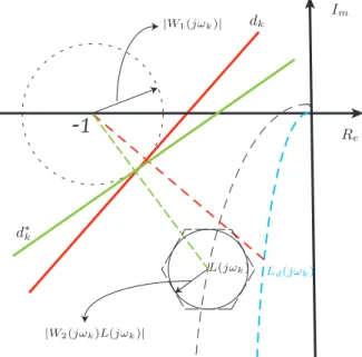
for k= 1, N (8) Note that|1 +L(jωk)| is the distance between the critical point and L(jωk). Hence, this constraint is satisfied if and only if there is no intersection in the Nyquist diagram between a circle centered at the critical point with a ra-dius of |W1(jωk)| and a circle centered at L(jωk) with a radius of |W2(jωk)L(jωk)| at each frequency ωk [8]. Now, consider a straight line d∗
k which is tangent to the circle with radius |W1(jωk)| and orthogonal to the line between the critical point andL(jωk). Therefore, the robust performance condition in (6) is satisfied if and only if the circle centered at L(jωk) does not intersect d∗
k and is completely in the side that excludes the critical point (at the right hand side in Fig. 1). This condition cannot be represented as a convex constraint becaused∗
kis a function of the controller parameters. However,d∗
k can be approximated bydk which is tangent to the circle with radius|W1(jωk)| but orthogonal to the line connecting the critical point to
Ld(jω) (see Fig. 1). It should be noted that the equation ofdk at each frequencyωk depends only onW1(jωk)and
Ld(jωk). If we name x and y, respectively, the real and imaginary parts of a point on the complex plane, the equation ofdk at each frequencyωk becomes :
|W1(jωk)[1 +Ld(jωk)]| −Im{Ld(jωk)}y−
[1 +Re{Ld(jωk)}][1 +x] = 0 (9) whereRe{·} andIm{·} represent real and imaginary parts of a complex value, respectively. Therefore, the condition that L(jωk) for all ωk is located in the side of dk that excludes the critical point can be given by the following linear constraints :
|W1(jωk)[1 +Ld(jωk)]| −Im{Ld(jωk)}ρTI(jωk)− [1+Re{Ld(jωk)}][1+ρTR(jωk)]<0 for k= 1, . . . , N
There exists two alternatives in order that this condition to be satisfied for all models in the uncertainty set represented by a circle centered at L(jωk). The first alternative is to approximate the uncertainty circle by a polygon of m >2 vertices. Then, the robust performance condition in (6) is
-1
|W1(jωk)| |W2(jωk)L(jωk)| Ld(jωk) d∗ k dk Re Im L(jωk)Fig. 1. Linear constraints for robust performance in Nyquist diagram
satisfied if all vertices are located in the right side of dk. This can be represented by the following constraints :
|W1(jωk)[1 +Ld(jωk)]| −Im{Ld(jωk)}ρTIi(jωk)− [1 +Re{Ld(jωk)}][1 +ρTRi(jωk)]<0
for k= 1, . . . , N and i= 1, . . . , m (10)
whereRi(jωk) andIi(jωk)are the real and the imaginary parts ofφ(jωk)Gi(jωk)with
Gi(jωk) =G(jωk)[1 + |
W2(jωk)| cosπ/m e
j2πi/m] (11)
It can be observed that the number of linear constraints are multiplied bymwhen the uncertainty circle is approximated by a polygon ofm vertices.
The second alternative is to consider for each frequency only one constraint for the closest point of the circle to
dk. It is clear that if this point is at the side of dk that excludes the critical point, then the whole uncertainty circle is in the correct side. The coordinates of the closest point of the uncertainty circle fromdk can be computed as :
x=ρTR(jωk)− |W2(jωk)ρTφ(jωk)G(jωk)| ×1 +Re{Ld(jωk)} |1 +Ld(jωk)| (12) y=ρTI(jωk)− |W 2(jωk)ρTφ(jωk)G(jωk)| ×Im{Ld(jωk)} |1 +Ld(jωk)| (13) Using these coordinates and the equation of dk in (9) the robust performance constraints obtained are no longer linear but convex with respect to the controller parameter vector
ρ:
|W1(jωk)[1 +Ld(jωk)]| −Im{Ld(jωk)}ρTI(jωk)+ |W2(jωk)ρTφ(jωk)G(jωk)[1 +Ld(jωk)]|−
[1 +Re{Ld(jωk)}][1 +ρTR(jωk)]<0
for k= 1, . . . , N (14) This alternative has less constraints and no conservatism but leads to a bit more complex convex optimization problem (convex constraints instead of linear constraints).
Remarks:
1) The same approach can be applied while an addi-tive uncertainty model is available. In this case the robust performance condition in (7) can be repre-sented by linear constraints in (10) or by convex con-straints in (14) with the difference that |W2(jωk)| = |W3(jωk)|/|G(jωk)|.
2) Individual shaping of the sensitivity functions is also possible using the constraints in (6) and (7) and putting one of the filters equal to zero. For example, in many applications we need to put some constraints on the magnitude of the input sensitivity function U(s) =
K(s)[1 +L(s)]−1in order to reduce the control effort. This can be done by defining a weighting frequency functionW3(jωk), usually a high pass filter, and using the constraints in (7) withW1(jω)≡0.
3) Multimodel uncertainty can be directly taken into account in the proposed approach. We only should repeat the constraints for each model in the model set. 4) The robust performance can be improved by defining
the following constraint :
k|W1S|+|W2T |k∞< γ (15) and minimizingγ. In the proposed approach an upper bound for γ can be computed by an iterative bisec-tion algorithm. At each iterabisec-tion for a fixed γi, we replace W1 and W2 with W1/γi and W2/γi and we solve the feasibility problem represented by the linear constraints in (10) or convex constraints in (14). If the problem is feasibleγi+1will be chosen smaller thanγi and if the problem is infeasibleγi+1 will be increased.
B. Optimization criterion
Up to now, it has been shown that the robust performance condition can be represented in the Nyquist diagram by a set of linear or convex constraints. Hence, fixed-order robust performance control problem becomes a feasibility problem with linear or convex constraints. The major drawback of the proposed approach with respect to the standard H∞ control problem is the need for a desired open-loop frequency functionLd(jω). However, it should be noted that the per-formance specification is defined by the weighting frequency function W1(jω) and Ld(jω) plays only an intermediate role to reduce the conservatism of the solution and not the solution itself. This means that even without knowing
Ld(jω), a straight line with a fixed slope for all frequencies can divide the Nyquist plane into two half planes and leads to a set of linear constraints for robust performance [6]. Therefore, Ld(jω) just adjusts the slope of dk to enlarge the set of admissible controllers defined by the constraints. As a result, a non properly chosen Ld(jω) may lead to a infeasible solution. By a non properly chosen Ld(jω) we mean a frequency function which is not coherent with the performance specification (with a bandwidth much larger than that specified byW1) and is far from achievable for the plant model with given uncertainty set and restricted order and structure of the controller. For example, if we consider an integrator in the controller but we do not put it inLd(jω) we will have evidently a non properly chosen Ld(jω). A suitable choice of Ld(jω) is a simple choice that satisfies the Nyquist stability criterion and has essentially the poles on the imaginary axis of the controller and the plant model. If Ld(jω)is chosen such that it represents some desired control specifications, then it is judicious to minimize a norm of L−Ld under the robust performance constraints. We propose either a quadratic programming approach in which an approximation of the two norm of L−Ld is minimized under some linear constraints :
min ρ N X k=1 |ρTφ(jωk)G(jωk)−Ld(jωk)|2 Subject to: |W1(jωk)[1 +Ld(jωk)]| −Im{Ld(jωk)}ρTIi(jωk)− [1 +Re{Ld(jωk)}][1 +ρTRi(jωk)]<0 for k= 1, . . . , N and i= 1, . . . , m (16) or a convex optimization approach in which an approxima-tion of the infinity norm ofL−Ldis minimized under some convex constraints : min ρ maxk |ρ Tφ(jωk)G(jωk) −Ld(jωk)| Subject to: |W1(jωk)[1 +Ld(jωk)]| −Im{Ld(jωk)}ρTI(jωk)+ |W2(jωk)ρTφ(jωk)G(jωk)[1 +Ld(jωk)]|− [1 +Re{Ld(jωk)}][1 +ρTR(jωk)]<0 for k= 1, . . . , N (17) It is interesting to notice that a large value of the criterion for the optimal solution shows that the choice of Ld(jω) has not been appropriate and with a better choice better performance may be achieved. Based on this observation a practical algorithm for improving the control performance can be suggested. We can start with a simple Ld(jω) and compute a first controller, sayK0(s), then we can compute a newLd(jω)equal toK0(jω)G(jω)and run the optimization problem with tighter specifications (e.g. larger|W1|). In this new optimization the conservatism is significantly reduced because LandLd and consequentlyd∗k anddk are close to each other at all frequencies.
C. Unstable systems
One of the main interest of the proposed approach with respect to other frequency-domain methods is that it can
be applied to the unstable systems. The essential condition is that the desired open-loop frequency function Ld(jω) should satisfy the Nyquist stability criterion. It means that
Ld(jω) has to encircle the critical point np times, where
np is the number of unstable poles of G(s) (knowing that the controller K(s) has no poles in the right half plane). Under this condition,L(jω) will encircle the critical point
np times too if the constraints in (10) or (14) are satisfied. The reason is as follows : ifLd(jω)encircles np times the critical point, then the vector1 +Ld(jω) anddk which is orthogonal to this vector will turnnptimes around the critical point. Hence, sinceL(jω)and all models in the uncertainty circle are always in the side ofdk that excludes the critical point, they will also encircle the critical pointnp times.
If the unstable poles of the plant model are known, a good choice ofLd(jω) includes these poles. If these poles are unknown,Ld(jω) should contain the same number of unstable poles as the plant model. Finally, if a stabiliz-ing controller K0(s) is known, an appropriate choice is
Ld(jω) =K0(jω)G(jω). In this case,Lddoes not represent a desired open-loop transfer function so it is not necessary to minimize a norm ofL−Ld in the optimization problem and only a feasibility problem can be solved instead.
IV. SIMULATION RESULTS
This example is taken from [10] where a robust perfor-mance problem is defined for an unstable plant. Consider the family of plants described by the following multiplicative uncertainty model: P(s) = (s+ 1)(s+ 10) (s+ 2)(s+ 4)(s−1)[1 + W2(s)∆(s)] (18) where W2(s) = 0.8 1.1337s2+ 6.8857s+ 9 (s+ 1)(s+ 10) (19) The nominal performance is defined bykW1Sk∞<1with :
W1(s) = 2
(20s+ 1)2 (20) The objective is to compute a controller K(s) that opti-mizes the robust performance by minimizingγin (15).
The standard H∞ solution that solves an approximate problem leads to γopt = 0.844 for this problem with the controllerK(s) =N∞/D∞ where N∞= 7.409e6s6+ 1.266e8s5+ 6.335e8s4+ 1.152e9s3 + 6.911e8s2+ 5.442e7s+ 9.37e5 (21) and D∞=s7+9.07e5s6+1.901e7s5+1.043e8s4+4.416e7s3 −4.682e7s2−4.962e6s−1.262e5 (22) This 7th-order controller is unstable and has a pair of complex conjugate poles very close to the imaginary axis.
Now, the proposed method is applied to design a PID controller represented by : K(s) = [Kp, Ki, Kd][1,1 s, s 1 +Tfs] T
where the time constant of the derivative part of the PID controllerTf is set to 0.01 s. The frequency response of the model is computed at N = 50 logarithmically spaced fre-quency points between10−3 and103rad/s. The uncertainty circle at each frequency is approximated by an outbounding polygon withm= 8vertices. The plant model contains one unstable pole and the controller an integrator, so the desired open-loop transfer function is chosen as
Ld(s) =β s+ 1
s(s−1) (23) where β > 1 satisfies the Nyquist stability condition for
Ld(s). In this example, we choose β = 2. It should be noted that this choice ofLd(s)is not compatible with desired performances so the difference betweenL(s)andLd(s)will not be minimized. In order to obtain the controller giving the minimal value for γ, the bisection algorithm explained in Remark 4 is used with the linear constraints in (10) that leads to
k|W1S|+|W2T |k∞= 0.7233 The resulting PID controller is :
K0(s) =
2.426s2+ 6.675s+ 11.11
0.01s2+s (24) It is interesting to observe that this PID controller gives better performance than the H∞ controller. Moreover, it is stable and easily implementable on a real system. The performance can be further improved using a newLd(s)based onK0(s). With this new Ld(s)the optimal controller is given by :
K(s) = 3.416s
2+ 26.28s+ 25.08
0.01s2+s (25) which leads to γopt= 0.7213.
In order to study the sensitivity of the solutions to the choice ofLd(s), the value ofβ in (23) is changed from 2 to 97 with a step size of 5. For each value ofβ the minimum ofγ is computed. The mean value of optimalγ’s is 0.7549 and its standard deviation 0.0228. This shows that although the optimal solution depends on the choice ofLd(s), it is not very sensitive to this choice. Moreover, the results obtained by this approach, whatever the choice of β between 2 and 97, are better than the standardH∞ optimal solution.
V. DISCUSSION
It should be mentioned that the problem of robust fixed-order controller design is a non-convex NP-hard problem and all solutions to this problem, including ours, are based on some approximations. For example, if we consider the standard H∞ control problem for design of a fixed-order controller for a system with multiple models and frequency-domain uncertainty, we have the following approximations : 1) Approximation of the structured multimodel uncer-tainty with unstructured frequency-domain unceruncer-tainty.
2) Approximation of the frequency-domain uncertainty with a reduced-order weighting filter.
3) Approximation of the real robust performance condi-tion in (4) with the condicondi-tion given in (5).
4) Approximation of the resulting high-order controller with a fixed-order controller. In this operation, it is dif-ficult to even guarantee the stability and performance for the reduced-order controller.
The proposed method considers directly the multimodel and frequency-domain uncertainty and designs directly a fixed-order controller. However, it seems that this method has some drawbacks which are discussed below :
1) The plant and uncertainties are defined only in N
frequency points, so the performance and stability conditions are satisfied only inN points. It is clear that
N should be sufficiently large such that the Nyquist diagram ofL(jωk)is a good approximation ofL(jω). For discrete-time controller design, since the frequency domain is limited to the half of sampling frequency, by increasingN the quality of approximation can be improved. This will increase the number of constraints but will not make a serious problem for linear and quadratic programming methods which are able to deal with more than hundred thousand of linear constraints. For continuous-time controller design, the choice ofN
and the sampling frequency should be done cautiously. This will need some information about the plant and the desired closed-loop specifications.
2) The controller is linearly parameterized so the denom-inator of the controller is fixed and it should be chosen prior to design. In practice, some of the poles of the controller are usually fixed to achieve certain closed-loop performances. For example a pole at origin, an integrator, or a pair of complex poles in a certain frequency are fixed in order to reject the disturbances (internal model principle). Therefore, this condition is not restrictive for low-order controller design. For higher order controller design the use of a set of orthogonal basis function is proposed. It is known that by increasing the controller order any stable transfer function can be approximated with such a set. On the other hand, this restriction ensures the stability of the controller which is required in many applications and cannot be guaranteed by a full controller parameteri-zation.
3) The robust performance condition in (4) is approxi-mated by a set of linear constraints in (10) or convex constraints in (14). It is discussed in the paper that the quality of this approximation depends on the choice of a desired open-loop transfer function.
It is too difficult (if not impossible) to compare, by a the-oretical analysis, the overall approximation or conservatism of different approaches to fixed-order controller design. In this paper we tried to show the effectiveness of the proposed approach by means of a simulation example and compare it with the standardH∞ method.
VI. CONCLUSIONS
A new fixed-order robust controller design method in the Nyquist diagram for spectral models has been developed. The method is based on an approximation of the robust per-formance condition in theH∞framework that leads to linear or convex constraints with respect to linearly parameterized controllers. The advantages of this approach are summarized below:
1) The method uses only the frequency response of the system and no parametric model is required. The frequency response of the model and the uncertainty at each frequency can be obtained directly by discrete Fourier transform from a set of periodic data, so the method can be considered as completely “data-driven”. Of course, the method can be applied as well if a parametric model with an uncertainty set is available. 2) The method is very simple, at least as simple as open-loop shaping methods in Bode diagram or in Nichols chart currently used in textbooks for undergraduate courses in control systems. For instance, it can be used to design of PID controllers ensuring a given modulus margin and optimizing for a desired crossover frequency by a quadratic programming optimization approach. Moreover, the case of multimodel uncer-tainty can be handled easily just by increasing the number of linear constraints while the mentioned clas-sical frequency-domain approaches cannot deal with this type of uncertainty.
3) Higher order controllers for unstable systems withH∞ type specifications can also be designed within the same framework.
REFERENCES
[1] I. M. Horowitz. Quantitative Feedback Theory (QFT). QFT Publica-tions Boulder, Colorado, 1993.
[2] G. F. Bryant and G. D. Halikias. Optimal loop shaping for systems with large parameter uncertainty via linear programming. International
Journal of Control, 62:557–568, 1995.
[3] G. D. Halikias, A. C. Zolotas, and R. Nandakumar. Design of optimal robust fixed-structure controllers using the quantitative feedback theory approach. Proceedings of the Institution of Mechanical Engineers, Part
I: Journal of Systems and Control Engineering, 221(4):697–716, 2007.
[4] E. Grassi and K. Tsakalis. PID controller tuning by frequency loop shaping. In 35th IEEE Conference on Decision and Control, pages 4776–4781, Kobe, Japan, 1996.
[5] E. Grassi, K. S. Tsakalis, S. V. Gaikwad S. Dash, W. MacArthur, and G. Stein. Integrated system identification and PID controller tuning by frequency loop-shaping. IEEE Transactions on Control Systems
Technology, 9(2):285–294, 2001.
[6] A. Karimi, M. Kunze, and R. Longchamp. Robust controller design by linear programming with application to a double-axis positioning system. Control Engineering Practice, 15(2):197–208, February 2007. [7] G. Galdos, A. Karimi, and R. Longchamp. Robust loop shaping controller design for spectral models by quadratic programming. In
46th IEEE Conference on Decision and Control, pages 171–176, New
Orleans, USA, 2007.
[8] C. J. Doyle, B. A. Francis, and A. R. Tannenbaum. Feedback Control
Theory. Mc Millan, New York, 1992.
[9] B. D. O. Anderson. Windsurfing approach to iterative control design. In P. Albertos and A. Sala, editors, Iterative Identification and Control:
Advances in Theory and Applications,. Springer-Verlag, Berlin, 2002.
[10] T. E. Djaferis. Robust Control Design: A Polynomial Approach.