Statistics Preprints Statistics
4-2015
A Multi-level Trend-Renewal Process for Modeling
Systems with Recurrence Data
Zhibing Xu
Virginia Tech
Yili Hong
Virginia Tech
William Q. Meeker
Iowa State University, [email protected]
Brock E. Osborn
GE Global Research Center
Kati Illouz
GE Global Research Center
Follow this and additional works at:http://lib.dr.iastate.edu/stat_las_preprints Part of theStatistics and Probability Commons
This Article is brought to you for free and open access by the Statistics at Iowa State University Digital Repository. It has been accepted for inclusion in Statistics Preprints by an authorized administrator of Iowa State University Digital Repository. For more information, please contact
Recommended Citation
Xu, Zhibing; Hong, Yili; Meeker, William Q.; Osborn, Brock E.; and Illouz, Kati, "A Multi-level Trend-Renewal Process for Modeling Systems with Recurrence Data" (2015).Statistics Preprints. 126.
A Multi-level Trend-Renewal Process for Modeling Systems with
Recurrence Data
Abstract
A repairable system is a system that can be restored to an operational state after a repair event. The system may experience multiple events over time, which are called recurrent events. To model the recurrent event data, the renewal process (RP), the nonhomogeneous Poisson process (NHPP), and the trend-renewal process (TRP) are often used. Compared to the RP and NHPP, the TRP is more flexible for modeling, because it includes both RP and NHPP as special cases. However, for a multi-level system (e.g., system, subsystem, and component levels), the original TRP model may not be adequate if the repair is effected by a subsystem replacement and if subsystem level replacement events affect the rate of occurrence of the component-level replacement events. In this paper, we propose a general class of models to describe replacement events in a multilevel repairable system by extending the TRP model. We also develop procedures for estimation of model parameters and prediction of future events based on historical data. The proposed model and method are validated by simulation studies and are illustrated by an industrial application.
Keywords
multi-level repairable systems, Nonhomogeneous Poisson process, renewal process, random effect, time-dependent covariate, trend-renewal process
Disciplines
Statistics and Probability
Comments
This preprint was published as Zhibing Xu, Yili Hong, William Q. Meeker, Brock E. Osborn, and Kati Illouz, "A Multi-level Trend-Renewal Process for Modeling Systems with Recurrence Data".
A Multi-level Trend-Renewal Process for Modeling
Systems with Recurrence Data
Zhibing Xu
1, Yili Hong
1, William Q. Meeker
2,
Brock E. Osborn
3, and Kati Illouz
3Abstract
A repairable system is a system that can be restored to an operational state after a repair event. The system may experience multiple events over time, which are called recurrent events. To model the recurrent event data, the renewal process (RP), the nonhomogeneous Poisson process (NHPP), and the trend-renewal process (TRP) are often used. Compared to the RP and NHPP, the TRP is more flexible for modeling, because it includes both RP and NHPP as special cases. However, for a multi-level system (e.g., system, subsystem, and component levels), the original TRP model may not be adequate if the repair is effected by a subsystem replacement and if subsystem-level replacement events affect the rate of occurrence of the component-subsystem-level replacement events. In this paper, we propose a general class of models to describe replacement events in a multi-level repairable system by extending the TRP model. We also develop procedures for estimation of model parameters and prediction of future events based on historical data. The proposed model and method are validated by simulation studies and are illustrated by an industrial application.
Key Words: Multi-level repairable systems, Nonhomogeneous Poisson process, Re-newal process, Random effect, Time-dependent covariate, Trend-reRe-newal process.
1
Zhibing Xu and Yili Hong are with the Department of Statistics, Virginia Tech, Blacksburg, VA, 24061, USA (e-mail: [email protected]; [email protected])
2
William Q. Meeker is with the Department of Statistics, Iowa State University, Ames, IA, 50011, USA (e-mail: [email protected])
3
Brock E. Osborn is formerly with and Kati Illouz is with the Applied Statistics Laboratory, GE Global Research Center, Niskayuna, NY, 12309, USA (e-mail: [email protected]; [email protected])
1
Introduction
1.1
Background
A repairable system is defined as a system that will be restored to an operational state after a repair. In practice, a repairable system may experience multiple replacement events at different levels over time. For example, we consider a repairable vehicle with three levels: system (e.g., a truck), subsystem (e.g., the truck engine), and component (e.g., the oil pump). The replacement events can be the replacement of the oil pump (may be new or refurbished) or the replacement of the entire engine (may be new or refurbished). For some other examples, the failure of a computer motherboard can be repaired by replacing the whole motherboard or just by replacing the failed capacitors on the motherboard. The failure of a gearbox can be repaired by replacing the whole gearbox or just by replacing the failed gear.
In this paper, we consider a two-level repairable system where repair events can occur at the subsystem level, or the component (within a subsystem) level. We focus on a specific subsystem (e.g., the engine) in a vehicle and a particular component within that subsystem (e.g., the oil pump), although a subsystem may have many components. In particular,
• The replacement of a subsystem is called a subsystem event. In this case, the system can only be fixed by a subsystem replacement.
• The replacement of a component is called a component event. In this case, the system is fixed by a component replacement.
Often, the failed subsystems or components are replaced with refurbished units that are not as good as new units. When the subsystem is replaced, of course, the components inside the subsystem will be replaced at the same time leading to a change of the risk of having a failure at the component level. This repair information at multiple levels is available through maintenance records. In addition to replacement event times, dynamic covariates, such as system usage information, loading, and shocks may also be available.
One important goal of the modeling of the replacement events is to do field failure pre-diction, which is useful for purposes such as prognostics, maintenance scheduling, and spare parts provisioning. Prediction of component replacement events is difficult when there are also subsystem replacements. The objective of this paper is to use replacement information at multiple levels and system usage information to make field failure predictions for a critical
component in a subsystem. We need a model that can incorporate the effects of system usage information and other possibly unobservable factors, and the effects that replacements at dif-ferent levels have on the component failure process. The model can also handle situations in which replacements may not be perfect and there are possible system-to-system differences.
1.2
Motivating Application
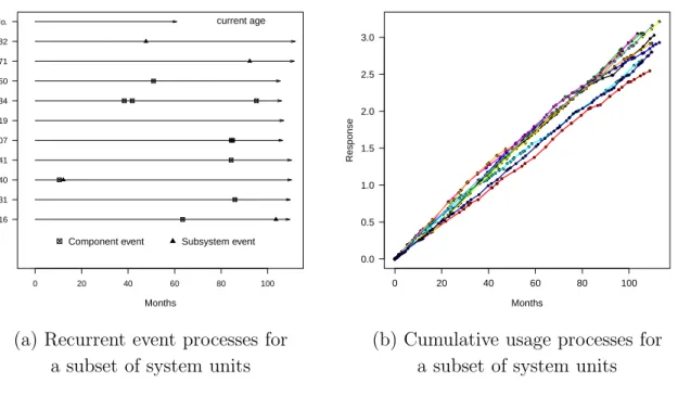
This paper is motivated by the need to model recurrent events from a fleet of industrial systems, which we call Vehicle B. Vehicle B is a two-level repairable system, and it may experience subsystem (engine) and component (oil pump) events over time. To protect sensitive and proprietary information, names, the scales of time and the covariates have been changed in the following analysis. There are n = 203 systems being tracked in the field, and the data freeze date (DFD) is around 110 months after the first installation. The total number of component events and subsystem events are 219 and 44, respectively. The event histories of ten randomly selected units from the Vehicle B fleet are shown in Figure 1(a).
In addition to the event histories, several time-dependent covariates were also recorded. All the covariates, however, have a strong linear relationship to each other indicating that after using one covariate, there is little or no additional information in the others. Thus we used the cumulative usage covariate. Figure 1(b) shows the cumulative usage for ten randomly selected units from the Vehicle B fleet. Compared to the length of running times of the systems, the time needed to effect a repair is ignorable and is assumed to be zero. A prediction of the total number of component events in a future time period is needed in this application.
1.3
Related Literature and This Work
The nonhomogeneous Poisson process (NHPP) and the renewal process (RP) are the two most commonly used models in the analysis of recurrent event data (e.g., Zhao and Liu 2003, Leemis 2004, and Hong et al. 2013) with the assumption that the effect of repair is perfect or minimal, respectively. For general repairs, Brown and Proschan (1983) proposed an imperfect repair model. Kijima (1989) introduced two types of virtual age models by reducing the age of the system after each repair. Lawless and Thiagarajah (1996) used a proportional intensity model to incorporate renewals and time trends. Wang and Pham (1996) proposed a quasi renewal process with the consideration of maintenance cost. Doyen and Gaudoin (2004) proposed two new classes of imperfect models.
Months 16 31 40 41 107 119 134 150 171 182 ID No. 0 20 40 60 80 100 current age
Component event Subsystem event
0 20 40 60 80 100 0.0 0.5 1.0 1.5 2.0 2.5 3.0 Months Response
(a) Recurrent event processes for (b) Cumulative usage processes for
a subset of system units a subset of system units
Figure 1: Plots of event processes and cumulative usage processes for ten randomly selected units in the Vehicle B fleet.
Lindqvist et al. (2003) and Lindqvist (2006) introduced a trend-renewal process (TRP) which includes the NHPP and RP as special cases. The TRP model has been widely used in the literature (e.g., Yang et al. 2012, and Pietzner and Wienke 2013). Heggland and Lindqvist (2007) derived the non-parametric maximum likelihood estimator of the intensity function for the TRP. Franz et al. (2013) proposed methods for point prediction and interval prediction for the first time to failure using simulation. For virtual age models, Ya´nez et al. (2002) and Yu et al. (2013) proposed methods to estimate the expected number of failures using Monte Carlo simulation and an analytic approach, respectively.
For multi-level repairable system analysis, some papers have focused on the reliability analysis of a system by combining information from different levels using Bayesian methods. Examples include Johnson et al. (2005), Wilson et al. (2006), and Liu et al. (2011). We know of no previous work that has been done for reliability estimation and prediction for multi-level repairable systems with the consideration of the effect of subsystem events on component events.
Motivated by the Vehicle B application, we propose a multi-level trend renewal process (MTRP) with time-dependent covariates in the modeling of component events. Based on the MTRP model, we also develop procedures for obtaining point predictions and prediction
intervals for the number of component events in a future time. To incorporate system-to-system variability, random effects are introduced in the MTRP model and the parameters are estimated by the Metropolis-within-Gibbs algorithm. Finite-sample properties of the estimators and prediction method are validated by simulation studies and illustrated with the Vehicle B application.
1.4
Overview
The rest of the paper is organized as follows. Section 2 introduces existing models and the proposed MTRP model. Section 3 develops estimation methods for the unknown parameters in the proposed MTRP model. Section 4 develops procedures for point predictions and prediction intervals (PI) based on Monte Carlo simulation. Section 5 validates the proposed methods by simulations. Section 6 illustrates the methods of modeling and predictions based on the Vehicle B application. Section 7 gives a summary and some related future research topics.
2
Repairable System Models
2.1
Existing Models
Let 0< T1· · · < Ti <· · · be the event times from a repairable system. Let N(t) denote the
counting process for the number of events that occur in time interval (0, t], and let Ft be the
event history up to time t. The event intensity for the counting process is
λ(t|Ft−) = lim
∆t→0
Pr{N(t+ ∆t)−N(t) = 1|Ft−}
∆t ,
where Ft− is the event history immediately prior to time t. The cumulative event intensity function is defined as Λ(t) =R0tλ(u|Fu−) du.
The RP, denoted by RP(F), corresponds to a perfect repair (i.e., replacement with a new unit), and the gaps between event times are independently and identically distributed (iid) withF. HereF is a cumulative distribution function (cdf). That is,Ti+1−Ti
iid
∼F, i= 1,2,· · ·. Let h(z) be the hazard function corresponding to F. The event intensity function of the RP is λ(t|Ft−) = h[t−TN(t−)], where TN(t−) is the last event time before time t. The NHPP corresponds to a minimal repair (e.g., adjustment or replacement of a small part of a large unit). The intensity function is λ(t|Ft−) =λ(t), which does not depend on the event history. For the NHPP, the transformed event times Λ(Ti) can be described by a homogeneous Poisson
process (HPP) with a mean of one. The gaps between the transformed times are iid with an exponential distribution with mean one. That is, Λ(Ti+1)−Λ(Ti)
iid
∼Exp(1), i= 1,2,· · · .
The TRP model describes situations that are in-between NHPP and RP, and contains the NHPP and RP models as special cases. The gaps between the transformed event times are iid with RP(F). That is, Λ(Ti+1)−Λ(Ti)
iid
∼ F, i = 1,2,· · ·. We denote the TRP by TRP(F, λ), where λ(t) = dΛ(t)/dt is called the trend function and F is called the renewal distribution function. The event intensity function is λ(t|Ft−) =h{Λ(t)−Λ[TN(t−)]}λ(t). The trend function λ(t) reflects system deterioration (or improvement) overtime, independent of replacement events or other repair-related events. The factorh{Λ(t)−Λ[TN(t−)]} reflects the effect of the most recent repair at time TN(t−). After each repair, there is a change in the event intensity function. The behavior of the change is determined by the hazard function of the renewal distribution function F.
2.2
Notation for Data
We consider a fleet of n multi-level repairable systems, which are under observation over the time interval (0, τi], where i= 1,· · · , n. The subsystem consists of many components and we
focus on the replacement of one particular critical component that had been carefully tracked. Let Ni(t) = Nis(t) +Nic(t) be the total number of replacement events up to time t, where
Nis(t) and Nic(t) are the number of subsystem events and the number of component events
up to time t for system i, respectively. Let 0 < ts
i1 < · · · < tsi,Nis(τi) < τi be the times for
subsystem events, and let 0< tc
i1 <· · ·< tci,Nic(τi) < τi be the times for component events. The
replacement event times, regardless of the types, are denoted by 0< ti1 <· · ·< ti,N(τi) < τi.
In the Vehicle B data, the time-dependent covariate (i.e., cumulative usage) at time t is denoted by Xi(t) for system i, where i= 1,· · · , n. The time-dependent covariate process for
system i is denoted by Xi(t), where Xi(t) = {Xi(u) : 0 < u ≤ t}. The covariate process Xi(t) is recorded at timetik, wherek = 1,· · · , mi, and mi is the number of time points where
the covariate information is available for system i before the end of observation τi.
With the consideration of the time-dependent covariate, the replacement events history up to time t isFt ={Nic(u), Nis(u), Xi(u) : 0 < u≤ t}, and the history of subsystem events up
to timet isFs
2.3
The Proposed Multi-level Trend-renewal Process
In a two-level repairable system i, the intensity functions for the subsystem and component level events are modeled as follows:
Subsystem level: λs⋆i (t|Fts−;θ s) =hs⋆ {Λ⋆i(t)−Λ⋆i[tsi,Nis(t−)];θ s }λ⋆i(t;θs), (1) Component level: λci(t|Ft−;θc) =hc Λsi(t|Fts−)−Λ s i ti,Ni(t−)| F s t− i,Ni(t−) ;θc λsi(t|Fts−;θ c). (2) In (1), we use a TRP model, TRP(Fs⋆, λ⋆
i), without random effects, to describe the
subsystem-level events. The unknown model parameters in (1) are denoted by θs. Here, we use “⋆” to
denote the functions used in the model for subsystem replacement events. LetFs⋆ denote the
renewal distribution for the subsystem-event process, hs⋆(·) denote the corresponding hazard
function, and Λ⋆ i(t) =
Rt
0 λ
⋆
i(u;θs)du denote the cumulative intensity function. The function
λ⋆
i(t;θs) =λ⋆b(t) exp{κg[Xi(t)]} is the intensity trend function for system i with λ⋆b(t) as the
baseline intensity function and κ as the coefficient of a transformed function of the time-dependent covariate (i.e., g[Xi(t)]). In the rest of this paper, we use g[Xi(t)] = log[Xi(t)] as
the function of the time-dependent covariate.
The proposed MTRP model for component events in (2) is an extension of the TRP in the sense that we use an additional trend function λs
i(t|Fts−;θ
c) for the component-event process
that can incorporate the effect of subsystem events on the component events, because the intensity of component events may be affected by the subsystem events. In particular,
λsi(t|Fts−;θ
c) =hs
{Λi(t)−Λi[tsi,Nis(t−)]}λi(t;θ
c), (3)
where θc = (θc
1,· · · , θpc)′ denotes a vector of unknown parameters with length of p in (2).
The function hs(·) in (3) describes the effect that subsystem events have on the intensity of
component events. As in (1), the form of hs(·) can be taken to be a hazard function, and its
corresponding cdf form is Fs(·). The function λ
i(t;θc) describes the effect of covariate and
other unknown factors on the component intensity function. Here, Λi(t) = Rt
0λi(u;θ
c) du.
The renewal distribution function of the component-event model in (2) is denoted by
Fc(·). We use fc(t), Sc(t) = 1 −Fc(t), and hc(t) to denote, respectively, the probability
density function (pdf), survival function, and hazard function corresponding to Fc. Also, let
Λs i(t|Fts−) = Rt 0 λ s i(u|Fus−;θ c)du, and Λ i(t) =R0tλi(u;θc)du. Note thatλsi(t|Fts−;θ c
) in (3) has the same parametric form of the TRP intensity model for subsystem events [i.e., λs⋆
i (t|Fts−;θ
s
of θs. The trend function λs
i(t|Fts−;θ
c) in (3) reflects the effect that subsystem events have
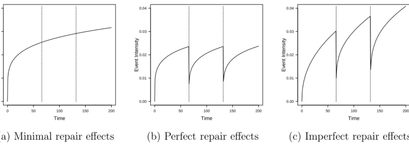
on the component-event intensity. For example, when hs(·) is a constant function, subsystem
events have no effect on components [e.g., Figure 2(a)]; when λi(t;θc) in (3) is a constant
function over time and hs(·) is not a constant function, a subsystem event corresponds to a
perfect repair and results in an immediate reduction of the intensity function [e.g., Figure 2(b)]; when neither λi(t;θc) nor hs(·) is a constant function, the subsystem events are imperfect
repairs [e.g., Figure 2(c)]. Thus, (3) is a flexible trend function for describing the effect that subsystem events have on the component-event intensity. Figure 3 illustrates the intensity function of component events in the MTRP model (2) for a simulated event history. In Figure 3, the intensity function of component events is affected by both the subsystem and component events.
Similar to the subsystem-event process, the incorporation of the time-dependent covariate can be achieved by
λi(t;θc) = λb(t) exp{γlog[Xi(t)]} i= 1,· · · , n. (4)
Here, λb(t) denotes the baseline intensity trend function if no component/subsystem
replace-ment events occur, and γ is the coefficient of the function of the time-dependent covariate. The MTRP with a time-dependent covariate can be denoted by MTRP(Fc, Fs, λ
i). We want
to point out that model (4) provides a flexible way of including time-dependent covariates into the event intensity function. Also, model (4) can be generalized, without difficulty, to include multiple time-dependent covariates.
To incorporate unit-to-unit variability in a component-event process, we use random effects in the intensity function (4) as follows,
λi(t;θc) =λb(t) exp{γlog[Xi(t)] +wi} i= 1,· · ·, n, (5)
where the random effect for system i, wi, is iid with N(0, σ2r). Here, σr2 is the variance of
the normal distribution, and is not contained in θc. Define w = (w1, w2,· · · , wn)′. The
heterogeneous MTRP for component events in system i is denoted by HMTRP(Fc, Fs, λ i).
2.4
Properties and Special Cases of MTRP
From another perspective, the MTRP model in (2) includes two TRP models in a hierarchical structure. The higher-level TRP model is used to describe the effect of subsystem events on
0 50 100 150 200 0.00 0.01 0.02 0.03 0.04 Time Ev ent Intensity 0 50 100 150 200 0.00 0.01 0.02 0.03 0.04 Time Ev ent Intensity 0 50 100 150 200 0.00 0.01 0.02 0.03 0.04 Time Ev ent Intensity
(a) Minimal repair effects (b) Perfect repair effects (c) Imperfect repair effects Figure 2: Different cases of the trend function in (3). The vertical dotted lines indicate the occurrence of subsystem event.
0 50 100 150 200 0.00 0.02 0.04 0.06 0.08 Time Ev ent Intensity
Figure 3: Illustration of the intensity function of component events in the MTRP model (2) for a simulated event history. The vertical solid (dashed) lines indicate the subsystem (component) event times.
the intensity of component events. The lower-level TRP model is used to model the component events with the higher-level TRP intensity function as its trend function. Thus, the MTRP can be defined as,
Λi(Ti,js +1)−Λi(Tijs) iid ∼Fs(·), Λs i(Tijc|FTsc ij−)−Λ s i " Ti,Ni(Tc ij−)| F s T− i,Ni(T c ij−) # iid ∼Fc(·), i= 1,· · · , n, j = 1,2,· · ·. For system i,Tc
ij is component event time j, andTNi(Tijc−) denotes the most recent event time
before Tc
ij. The cumulative intensity function for component events is computed as
Λci(t|Ft−) = Z t 0 λci(u|Fu−;θc) du =Hc Λsi(t|Fts−)−Λ s i[ti,Ni(t−)|F s t− i,N(t−) ] + NXi(t−) j=1 HchΛsi(tij|Fts− ij)−Λ s i(ti,j−1|Fts− i,j−1 )i,
where Hc(t) = R0thc(u) du is the cumulative hazard function corresponding to Fc.
The MTRP model is a general model that includes the TRP, RP, NHPP and HPP models as special cases. Here, the application of the special cases, TRP, RP, NHPP, and HPP models, are slightly different from the usual application of these models because subsystem events induce censoring during system operation. For example, if a subsystem is replaced, then observation is terminated on the components in that subsystem. The intensity function (2) of the MTRP model reduces to the TRP model if hs(·) is a constant function indicating
no subsystem repair effect (i.e., only minimal repair effects from subsystem events). When both hs(·) and λ
i(t;θc) are constant functions, the MTRP model reduces to the RP model,
indicating that subsystem events have no effect on component events, and component events are perfect repairs. When hc(·), and hs(·) are constant functions and λ
i(t;θc) is a function
of t, the MTRP model reduces to an NHPP model, indicating component events are minimal repairs and there are no subsystem-event effects. When Fc(·) is an Exp(1) distribution and
both hs(·) and λ
i(t;θc) are constant functions, the MTRP model reduces to the HPP model.
The likelihood ratio test can be used in the comparison and selection of these nested models. More details on the subject of model selection in the context of the TRP model can be found in Lindqvist et al. (2003).
3
Parameter Estimation
The estimate of parameter θs in (1) can be obtained by using the method of Lindqvist et al.
(2003). So we focus on the estimation of the parameters in the component-event model in (2).
3.1
The Likelihood Function
Note that component events for system i follow MTRP(Fc, Fs, λ
i). For convenience in the
expression of the likelihood function, the component events are denoted by {tij, δijc}, where
i = 1,· · · , n, and j = 1,· · · , Ni(τi). Here, tij is the event time for system i, and δcij is
the component-event indicator. If the replacement is for a component, then the indicator is equal to one, and zero otherwise. Let ti0 = 0, ti,Ni(τi)+1 = τi, Λ
c
i(0|F0) = Λsi(0|F0s) = 0,
δc
i,Ni(τi)+1 = 0, and F = {Nic(u), Nis(u), Xi(u) : 0 < u ≤ τi, i = 1,· · · , n}. The likelihood
function for component events in the MTRP model can be expressed as
L(θc;F) = n Y i=1 NiY(τi)+1 j=1 [λci(tij|Ft− ij; θc)]δcij ×exp[−Λ c i(τi|Fτ− i )] = n Y i=1 Ni(Yτi)+1 j=1 n fc[Λsi(tij|Fts− ij)−Λ s i(ti,j−1|Fts− i,j−1)]λ s i(tij|Fts− ij; θc)oδ c ij ×nSc[Λsi(tij|Fts− ij)−Λ s i(ti,j−1|Fts− i,j−1 )]o1−δ c ij . (6)
3.2
Estimation Procedure
We first discuss the estimation procedure for the unknown parameters in the model with random effects (i.e., HMTRP). Bayesian methods using diffuse prior distributions provide a convenient method to obtain the estimates of the unknown parameters. We suggest a Metropolis-within-Gibbs algorithm because some conditional distributions do not have closed forms. Define υ = 1/σ2
r as the precision of the random effects distribution, and let υ ∼ Gamma(a1, a2) be the conjugate prior distribution for the random effects. Here, a1 is the
shape parameter and a2 is the rate parameter of a gamma distribution. Gelman (2006) and
DePalma (2013) suggested using 0.001 for botha1 and a2. Then the mean and variance of the
prior distribution ofυ are 1 and 1000, respectively. We use a uniform distribution to describe the prior information on θc. Define Li(θc|Fτ
i, wi) as the conditional likelihood function of
likelihood function for alln systems. Then, the pdf of the full joint distribution of parameters in the MTRP model is
P(θc,w, υ|F)∝L(θc|F,w)P(w|υ)P(υ), (7)
where P(w|υ) is the pdf of a multivariate normal distribution with mean 0 and
variance-covariance matrix Σr. That is w∼N(0,Σr =I/υ), where I is ann×n identity matrix. The
pdf of Gamma(a1, a2) is denoted byP(υ). Based on the full joint distribution, we can obtain
the joint posterior distribution of the parameters in the model as follows,
wi|θc, υ ∝Li(θc|Fτi, wi)υ 1/2exp −υw 2 i 2 (8) υ|w,θc ∝Gamma n 2 +a1, w′w 2 +a2 (9) θc|w, υ ∝L(θc|F,w). (10) Algorithm 1:
1. Initialize all the parametersw(0), υ(0) and θc(0);
2. Update wi(j), i= 1,· · · , n using Metropolis algorithm at step j: a) Sample w∗
i ∼N(wi(j−1), σw2i), where σ
2
wi is the variance of the proposed distribution
for unit i; b) Accept w∗
i as w
(j)
i with the probability
min Li(θc(j−1)|Fτi,w∗i)exp −υ (j−1)w∗2 i 2 Li θc(j−1)|F τi,w(ij−1) exp −υ (j−1)w(ij−1) 2 2 ,1 , otherwise, set w(ij) =w(ij−1). 3. Sample υ(j) ∼Gamma n/2 +a1,w(j) ′ w(j)/2 +a2;
4. Update values of elements of θc(j) = (θc(j)
1 ,· · · , θ c(j) i ,· · · , θ c(j) p )′ successively at step j. Letθc(j) i−1 = (θ c(j) 1 ,· · · , θ c(j) i−1, θ c(j−1) i ,· · · , θ c(j−1) p )′. Note that θ0c(j)=θc(j−1). a) Sample θc∗ i ∼ N(θci(j−1), σθ2c i), where σ 2 θc
i is the variance of the proposed distribution.
Letθc∗ i = (θ c(j) 1 ,· · · , θ c(j) i−1, θci∗, θ c(j−1) i+1 ,· · ·, θ c(j−1) p )′. b) Accept θc∗ i as θ c(j) i in θ c(j)
i with the probability
min L[θc∗ i |F,w(j)] L[θc(j)|F,w(j)],1 , otherwise, set θci(j)=θic(j−1) inθc(j) i .
c) Repeat steps a) and b) fori= 1,· · ·, p at the given j. Let θc(j) =θc(j)
p .
5. Repeat steps 2-4 until a large number (e.g., 10,000) draws from the joint posterior distribution have been obtained.
To achieve optimal acceptance rates (around .44 according to Gelman et al. 1997 and Roberts and Rosenthal 2001), the tuning parameters σwi and σθic, i = 1,· · · , p can be adjusted by
applying the method given in Roberts and Rosenthal (2009).
For a model without random effects (MTRP),Algorithm 1 can still be used by omitting steps 1-3. With no random effect parameters, however, it is straightforward to estimate the unknown parameters by using the maximum likelihood (ML) method based on the likelihood function (6).
Once the parameters estimates in the MTRP/HMTRP model are obtained, the residuals of the model can be estimated by using the cumulative hazard function. Specifically, the residuals can be estimated by evaluating Rij = Hc[Λsi(tij|Fts−
ij
)−Λs
i(ti,j−1|Fts−
i,j−1
)] using the values of the parameter estimates. The residuals (Rij, δcij = 1) are expected to behave as
samples from the Exp(1) distribution, which can be used to evaluate the goodness of fit of the model.
4
Prediction for Component Events
4.1
Point Prediction
Accurate prediction of future events is important to product manufacturers who provide ser-vice contracts, or to the operators of fleets of systems, for purposes of controlling operating costs, optimizing the number of spare components, and assessing the risk of excessive repair expenses or warranty returns. Here, we focus on the prediction of events at the component level.
Let θx denote the parameters in the model for the time-dependent covariate, and let Xi(t1, t2) = {Xi(t); t1 < t≤ t2}. The predicted cumulative number of component events in
the future time period t∗ for a fleet of n units can be obtained by: Nc(t∗;θc,θs,θx) = n X i=1 Nic(t∗;θc,θs,θx) = n X i=1 EXi(τi,τi+t∗)|X(τi)Ewi Nic[t∗,Xi(τi, τi+t∗), wi;θc,θs,θx] , (11)
where Nic(t∗;θc,θs,θx) is the predicted cumulative number of component events in system
i in the future time period t∗. Because the trend function of the component-event intensity depends on the history of subsystem events, the component-event model will also depend on the subsystem-event model. Hence, the prediction of component events will depend on the parameter vector of the subsystem-event model, θs. Because a closed form for (11) is not
available, numerical methods or Monte Carlo simulation must be used. For prediction in the general recurrent process, Monte Carlo simulation is more common and easier for computation as illustrated in Ya´nez et al. (2002) and Franz et al. (2013).
The simulation of Nc(t∗;θc,θs,θx) can be achieved by using the following steps.
• Simulate the time-dependent covariates;
• Simulate the subsystem events with the TRP model;
• Simulate the component events with the MTRP/HMTRP model.
4.2
Prediction for the Time-Dependent Covariate
To predict future recurrent events for a system with a time-dependent covariate, it is necessary to have a parametric model for the covariate process. Based on the covariate pattern shown in Figure 1(b), we use a linear mixed effects model to describe the dynamic covariate data. In particular,
Xi(tik) = tik(βx+νi) +ǫi(tik) i= 1,· · ·, n, k = 1,· · ·, mi, (12)
where βx is the coefficient of time, νi is the random effect, and ǫi(tik) is the error term. We
assume that νi iid ∼ N(0, σ2 ν), and ǫi(tik) iid ∼ N(0, σ2
x) is independent of νi. The parameters in
(12) are denoted by θx = (βx, σν, σx)′. The estimation of θx in the covariate model can be
accomplished by using existing software packages (e.g., using the R functionlme).
We use an approach that is similar to that used by Hong and Meeker (2013) for the covariate prediction for a different kind of failure-time model. Let ti = (ti1,· · · , tim)′,
tit∗ = (ti,mi+1,· · ·, ti,mi+zi)′ be the observed time points before τi and the predicted time points during (τi, τi + t∗], respectively. Let Xi(ti) = [Xi(ti1),· · · , Xi(timi)]
′, X
i(tit∗) = [Xi(ti,mi+1),· · · , Xi(ti,mi+zi)]
′ be the corresponding time-dependent covariate processes. Here,
zi is the number of predicted time points for system i. The joint distribution of Xi(ti) and
Xi(tit∗) can be expressed as " Xi(ti) Xi(tit∗) # ∼N " ti tit∗ ! βx, Σi11 Σi12 Σi21 Σi22 !# , where Σi11=σ2 νtit′i+σx2Imi, Σi22=σ 2 νtit∗t′it∗ +σ 2 xIzi, and Σi12 =σ 2 νtit′it∗. Here, Imi and Izi
are mi×mi and zi×zi identity matrices. The conditional distribution of Xi(ti)|Xi(tit∗) is N
tit∗βx+Σi21Σi−111[Xi(ti)−tiβx], Σi22−Σi21Σ−i111Σi12
. (13) The derivation of (13) is given in Appendix A. Based on (13), the time-dependent covariate processes can be predicted.
4.3
Subsystem Event Simulations
Because the model for component events depends on the history of subsystem events, the simulation of subsystem events is needed in the prediction of component events. Letςi =τi+t∗
be the prediction ending time of system i,Fbs⋆ be the estimate of renewal distribution function
Fs⋆,Λb⋆
i be the estimate of Λ⋆i, andΛb⋆i−1(·) be the corresponding inverse function given bθ s
and
b
θx. Here, θbs and θbx are ML estimates of θs and θx, respectively. Based on the definition of
the TRP model, the gaps between two consecutive transformed subsystem event times follow distributionFs⋆. That is, Λ⋆
i(tsi,j+1)−Λ⋆i(tsij)
iid
∼Fs⋆, where i= 1,· · · , nand j = 1,2,· · ·. The
subsystem events can be simulated as follows. Algorithm 2
1. Simulate a realization of Xi(tit∗), the ith time-dependent covariate process, based on
b
θx using the conditional distribution (13).
2. Compute Λb⋆
i(ςi) as the prediction ending time for unit i.
3. Generate a sequence of random variables Uij from distribution Fbs⋆ and obtain the
se-quence of simulated event times in a transformed time scale,Tij∗ =Λb⋆i[tsi,Nis(τi)]+
Pj k=1Uik, j = 1,· · · , Cs i, until Ti,C∗ s i+1 > Λb ⋆
the transformed time scale according to the RP(Fs⋆) model. Then, Cs
i is the random
number of simulated subsystem events for unit i. 4. Compute the simulated subsystem event times Ts
ij =Λb⋆i−1(Tij∗), j = 1,· · · , Cis.
5. Repeat steps 1-4 for each system i, where i= 1,· · · , n.
Note that in step 3, the time of the first simulated subsystem event Ts
i1 should be larger than
τi, because the simulation is conditioned on the history. Otherwise it needs to be re-simulated.
4.4
Computation of Point Predictions
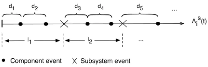
According to the definition of the MTRP model, the gaps (i.e., d1, d2,· · ·) between the
com-ponent event and the most recent event (either comcom-ponent event or subsystem event) in the transformed time scale [i.e., Λs(t)] follow the Fc distribution as shown in Figure 4. Because
the component-event process is censored by the subsystem events, the component events can be simulated in the intervals (i.e., I1, I2, ... in Figure 4) of the subsystem events under the
transformed time [i.e., Λs(t)] scale. In particular, for each system,
Λsi(Tijc|FTsc ij−)−Λ s i " Ti,Ni(Tc ij−)| F s T− i,Ni(T c ij−) # iid ∼Fc(·),
where i = 1,· · · , n and j = 1,2,· · ·. Let bθc and υb be the mean of posterior distributions
of θc and υ, respectively. The prediction of the cumulative number of component events,
b
Nc(t∗;θb c
,θbs,θbx), can be computed by using the following algorithm.
Algorithm 3
1. Repeat Algorithm 2 steps 1-4. Then the predicted covariate process and simulated times of subsystem events for system i are obtained. The simulated subsystem events times are denoted by ts
i,Nis(τi)+1,· · ·, t s
i,Nis(τi)+Cis. Here C s
i is the simulated number of
subsystem events. Set ts
i,Nis(τi)+0=t s
i,Nis(τi) and t s
i,Nis(τi)+Csi+1 =ςi.
2. The random effect wi can be obtained by the Metropolis algorithm. The conditional pdf
of wi is proportional to the product ofLi
b
θc|Ft, wi and P(wi|bθc,bυ). For the MTRP
d1 d2 d3 d4 d5 ...
I1 I2 ...
Λis(t)
Component event Subsystem event
Figure 4: Illustration of the component event simulation.
3. Calculate the simulated time intervals which are separated by the simulated subsystem events for system i in the transformed time scale. That is Iik = ΛbsibΛi(tsi,Nis(τi)+k)− b
Λs
ibΛi(tsi,Nis(τi)+k−1)
, k = 1,· · · , Cs
i + 1, where Λbsi(·) andΛbi(·) are the estimates of Λsi(·)
and Λi(·) based on the estimates bθ c
and θbx, respectively.
4. For each simulated time interval, generate random variables Uikl from distribution Fbc,
while PlUikl≤Iik. The number of generated Uikl values is recorded asCikc .
5. Calculate the number of simulated component events in system i. That is Cc
i =
PCi+1 k=1 Cikc.
6. Repeat steps 1-5 for each system i, where i= 1,· · · , n.
7. Repeat steps 1-6 B times and a series of Cic(b), b = 1,· · ·, B, i = 1,· · ·, n are ob-tained. Then, the point prediction for the number of events between τi and τi +t∗ is
b Nc(t∗;θb c ,bθs,θbx) =Pn i=1 PB b=1C c(b) i /B.
Note that in step 4 the time of the first simulated component event should be larger than τi.
Otherwise it needs to be re-simulated.
4.5
Prediction Interval Computing
In order to obtain PIs for the cumulative number of events, we also need to take into account the distribution of estimated parameters as well as the uncertainty in the future values of the time-dependent covariate. Instead of sampling the posterior distributions, we use a multivariate normal distribution to approximate the distributions of the parameter estimators for fast computing. We focus on the PI for the cumulative number of component events. The algorithm is described as follows.
Algorithm 4
1. Simulate θbx∗, θbs∗, bθc∗, and υb∗ from N(bθx,Σbb
θx), N(bθ s ,Σbθbs), N(bθ c ,Σbbθc) and N(υ,b bσ2 b υ), respectively.
2. Replacebθxbybθx∗,bθsbybθs∗,bθc bybθc∗, andbυbybυ∗, and repeat steps 1-7 inAlgorithm 3
to obtain Nb∗
c(t∗;θb c∗
,θbs∗,bθx∗).
3. Repeat steps 1-2 B times to obtain Nbc∗(b)(t∗;bθ c∗
,bθs∗,bθx∗), where b= 1,· · ·, B.
4. The 100(1−α)% PI for Nc is the (α/2,1−α/2) quantile of the B ordered values of b
Nc∗(b)(t∗;bθ c∗
,θbs∗,bθx∗).
5
Finite-Sample Performance of Estimation Methods
In this section, we use simulation to study the effect that sample size and number of events has on the performance of the estimation methods.
5.1
Design of Simulations
In the simulation, time is defined as the calendar time of system, and the time for repair is ignored. Only one time-dependent covariate is considered with the form of (12) and 30 time points per system. The parameter settings are θx = (βx, σν, σx)′ = (0.02,0.004,0.05)′ which
are similar to the Vehicle B application.
The subsystem events follow a TRP model with trend function λ⋆
i(t;θs) =
ata−1exp{κlog[X
i(t)]}and the renewal distribution function Fs⋆. We set Fs⋆ to be a Weibull
distribution and the corresponding hazard function is h⋆(t) = (β/η)(t/η)β−1, where η is the
scale parameter (also the approximate 0.63 quantile) and β is the shape parameter. Because the mean of renewal function is restricted to one, the corresponding hazard function can be expressed as h⋆(t) = Γ(1 +σ)σ1t 1 σ−1 1 σ , (14)
where σ = 1/β. The parameters for the subsystem areθs = (a, σ, κ)′ = (0.3,0.8,0.8)′.
Given the above simulated subsystem events, the simulation of component events is based on the HMTRP model with the consideration of time-dependent covariate and random effects.
Letλb = (α/ϕ)(t/ϕ)α−1. The trend function of system i in (5) can be denoted by λi(t;θc) =
(α/ϕ)(t/ϕ)α−1exp{γlog[X
i(t)] +wi}, where wi ∼ N(0, σ2r). Here, ϕ is set to be one in the
HMTRP model. The renewal distributions for the subsystem Fs and the component Fc are
both Weibull distributions with mean one. The mean-one restriction is used so that all model parameters are identifiable (Lindqvist et al. 2003). Similar to (14), the hazard functions can be expressed as hc(t) = Γ(1 + σ
0)1/σ0t1/σ0−1(1/σ0), and hs(t) = Γ(1 + σ1)1/σ1t1/σ1−1(1/σ1),
respectively. Then the intensity function of HMTRP can be expressed as
λci(t|Ft−) = hc Λsi(t|Fts−)−Λ s i ti,Ni(t−)| F s t− i,Ni(t−) hs Λi(t)−Λi[tsi,Nis(t−)] λi(t;θc), (15) where λi(t;θc) = (α/ϕ)(t/ϕ)α−1exp{γlog[Xi(t)] +wi}.
The parameters for the component-event intensity areθc = (α, σ0, σ1, γ)′ = (0.4,0.6,0.75,0.9)′
and σr = 0.5.
The number of systems n was selected to be 50, 100, and 200. For each value of n, we simulated data 1000 times based on the parameter settings. By selecting different DFDs, the expected number of subsystem events (q1) and component events (q2) in each sample size (i.e.,
n = 50,100, and 200) were controlled to the following three combinations (q1, q2): (0.7, 1.3),
(1.7, 4.3), and (3.9, 12.7).
5.2
Simulation Results
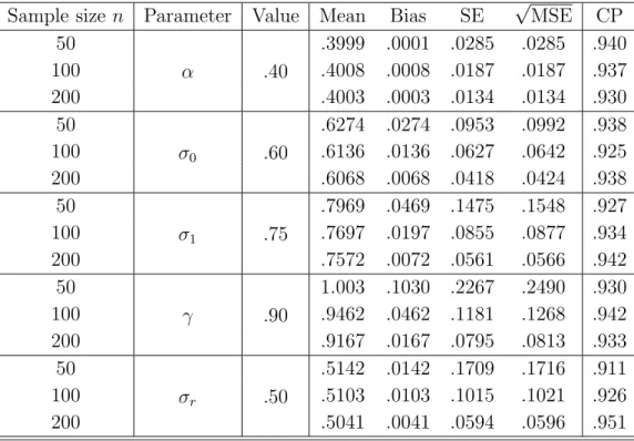
Based on theAlgorithm 1, the estimated parameters and corresponding standard errors (SE) for the component-event model were obtained and are shown in Tables 1-3. In the results, the estimates are close to the true values of the parameters, and they are approximately equal to the true settings as the sample size (n) and the length of study time (DFD) increase. Also, the coverage probability (CP) of the confidence interval procedure for each parameter is close to the nominal value of 0.95. The results show that our proposed estimation procedure can estimate the parameters well.
6
Application for the Vehicle B Data
In this section, we use the Vehicle B data to illustrate our proposed method for estimation and prediction of component events. Considering that the difference of the number of
com-Table 1: Summary of the simulation studies of the HMTRP given average number of subsystem events q1 = 0.7 and component events q2 = 1.3. Here “SE” stands for “standard error”, and
“CP” stands for “coverage probability”.
Sample size n Parameter Value Mean Bias SE √MSE CP
50 α .40 .3999 .0001 .0285 .0285 .940 100 .4008 .0008 .0187 .0187 .937 200 .4003 .0003 .0134 .0134 .930 50 σ0 .60 .6274 .0274 .0953 .0992 .938 100 .6136 .0136 .0627 .0642 .925 200 .6068 .0068 .0418 .0424 .938 50 σ1 .75 .7969 .0469 .1475 .1548 .927 100 .7697 .0197 .0855 .0877 .934 200 .7572 .0072 .0561 .0566 .942 50 γ .90 1.003 .1030 .2267 .2490 .930 100 .9462 .0462 .1181 .1268 .942 200 .9167 .0167 .0795 .0813 .933 50 σr .50 .5142 .0142 .1709 .1716 .911 100 .5103 .0103 .1015 .1021 .926 200 .5041 .0041 .0594 .0596 .951
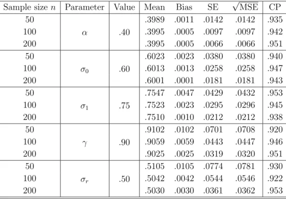
Table 2: Summary of the simulation studies of the HMTRP given average number of subsystem events q1 = 1.7 and component events q2 = 4.3. Here “SE” stands for “standard error”, and
“CP” stands for “coverage probability”.
Sample size n Parameter Value Mean Bias SE √MSE CP
50 α .40 .3989 .0011 .0142 .0142 .935 100 .3995 .0005 .0097 .0097 .942 200 .3995 .0005 .0066 .0066 .951 50 σ0 .60 .6023 .0023 .0380 .0380 .940 100 .6013 .0013 .0258 .0258 .947 200 .6001 .0001 .0181 .0181 .943 50 σ1 .75 .7547 .0047 .0429 .0432 .953 100 .7523 .0023 .0295 .0296 .945 200 .7510 .0010 .0212 .0212 .938 50 γ .90 .9102 .0102 .0701 .0708 .920 100 .9059 .0059 .0443 .0447 .946 200 .9025 .0025 .0319 .0320 .951 50 σr .50 .5105 .0105 .0774 .0781 .930 100 .5042 .0042 .0544 .0546 .922 200 .5030 .0030 .0361 .0362 .953
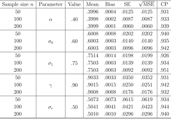
Table 3: Summary of the simulation studies of the HMTRP given average number of subsystem events q1 = 3.9 and component events q2 = 12.7. Here “SE” stands for “standard error”, and
“CP” stands for “coverage probability”.
Sample size n Parameter Value Mean Bias SE √MSE CP
50 α .40 .3996 .0004 .0125 .0125 .931 100 .3998 .0002 .0087 .0087 .933 200 .3999 .0001 .0060 .0060 .939 50 σ0 .60 .6008 .0008 .0202 .0202 .940 100 .6003 .0003 .0140 .0140 .935 200 .6003 .0003 .0096 .0096 .942 50 σ1 .75 .7514 .0014 .0198 .0199 .926 100 .7503 .0003 .0139 .0139 .934 200 .7503 .0003 .0092 .0092 .951 50 γ .90 .9033 .0033 .0350 .0352 .931 100 .9015 .0015 .0250 .0251 .942 200 .9008 .0008 .0176 .0176 .932 50 σr .50 .5073 .0073 .0615 .0619 .934 100 .5041 .0041 .0421 .0423 .944 200 .5010 .0010 .0296 .0296 .940
ponent events among different units is small, we assume that the prior distribution P(υ) is Gamma(a1, a2) with a1 = 10 and a2 = 0.06 in the HMTRP model indicating a small mean of
σr = 1/√υ. The intensity function of the component events in the HMTRP model is similar
to (15) using a Weibull distribution as renewal functions forFc and Fs. We fit the subsystem
events with the TRP model using λ⋆
i(t;θs) = ata−1exp{κlog[Xi(t)]} as trend function and a
Weibull distribution for the renewal function (Fs⋆).
6.1
Parameter Estimation
Table 4 lists the estimates and standard errors of parameters in the covariate model (12), subsystem-event model and component-event models. The Vehicle B data is also fitted by the HMTRP sub-models (i.e., HTRP, HRP and HNHPP). In the TRP model of subsystem events, the value of the Weibull shape parameter 1/σ is greater than one indicating the trend of the hazard function corresponding to the renewal function is increasing for subsystem events.
For the component events, several sub-models are compared to the HMTRP model. We use the deviance information criterion (DIC) as a criterion for Bayesian model selection. Sim-ilar to the Akaike information criterion (AIC), it considers both model adequacy and model complexity. Define the deviance as D(θ) = −2 log[f(y|θ)] + 2 log[g(y)], where θ denotes the
vector of unknown parameters, f(y|θ) is the likelihood function and g(y) is a standardizing
term. Then, the DIC can be expressed as DIC = ¯D+pD, where ¯D indicates the goodness of
fit with the form of ¯D=Eθ|y[D(θ)] =Eθ|y[−2 lnf(y|θ)] by settingg(y) = 1, andpD indicates
the penalty for model complexity with the form pD = ¯D−D(¯θ). Here, ¯θ is the posterior
mean of θ. By simple transformation, DIC can be re-expressed as DIC = D(¯θ) + 2pD, which
is similar to the form of AIC. More information about DIC can be found in Spiegelhalter et al. (2002), and Berg et al. (2004).
The DIC is easy to compute via the MCMC method. The estimate of ¯D and pD can be
computed by ¯D = PBb=1[−2L(θc(b)|Ft,w(b))]/B and pD = ¯D−[−2L(θbc|Ft,wb)] with θbc =
PB b=1θ c(b) /B and wb = PB b=1w(b)/B, respectively. Here, θ c(b)
and w(b) are the simulated
posterior estimates after burn in. The results of DIC in Table 4 show that the HMTRP model fits the data better than other sub-models because of the smallest value of DIC. However, the fit of the HMTRP model is just slightly better than the HTRP model due to the small number of subsystem events and component events. The value of 1/σ1 is larger than one, indicating
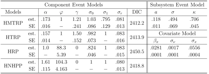
Table 4: Parameter estimates and standard errors for the component-event, subsystem-event, and covariate models, based on the Vehicle B data.
Component Event Models Subsystem Event Model
Models α ϕ γ σ0 σ1 σr DIC a σ κ
HMTRP est. .173 1 1.21 1.03 .795 .081 2412.2 .118 .494 .706
SE .016 − .241 .086 .129 .013 .011 .069 .045
HTRP est. .157 1 1.50 .982 1 .083 2413.9 Covariate Model
SE .014 − .152 .073 − .016 βx σν σx
HRP est. 1.0 88.3 0 .824 1 .083 2450.5 .0281 .0017 .0556
SE − 5.39 − .046 − .015 .0001 .0001 .0004
HNHPP est. 1.61 104.3 0 1 1 .080 2418.8
SE .115 4.163 − − − .013
intensity trend of component events. The value of 1/σ0 is close to one indicating that the
replacement of a component does not change the intensity trend of component events (i.e., minimal repairs).
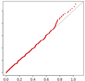
To check the goodness of fit of the model, we can use the Cox-Snell residual plot. The estimated residuals Rbij (with δijc as the censoring indicator) are expected to behave like a
censored sample from an Exp(1) distribution. Figure 5 is a Cox-Snell residual plot which shows that the HMTRP model provides a good fit to the data, as most of the points align well with the diagonal line.
6.2
Prediction Results
The cumulative number of component events is shown in Figure 6. From Figure 6, we observe that the trend of the increase of component events drops down in the last 10 months. This is due to the occurrence of the scheduled subsystem replacements which can be requested by the customers after usage covariate has reached a critical value according to the system service plan. There were 132 scheduled subsystem events during the last 15 months before the DFD.
The model in (1) only describes the unscheduled (randomly occurred) subsystem events. For prediction, it is important to incorporate the effect of scheduled subsystem events because it also affects the component-event intensity. After some exploratory analysis, we found that the scheduled subsystem event times T can be modeled adequately by a lognormal distribu-tion. Specifically, log(T)∼N(µ∗, σ∗2), where µ∗ and σ∗ are the location parameter and scale
0.0 0.2 0.4 0.6 0.8 1.0 0.0 0.2 0.4 0.6 0.8 1.0 Residuals T ransf or med Residuals
Figure 5: Residual plot for HMTRP model and the Vehicle B data.
parameter for the distribution of log(T), respectively. The ML estimates are µb∗ = 1.026 and
b
σ∗ = 0.115.
However, in the validation of the prediction algorithm, we setτi back 15 months to obtain
the subset of the Vehicle B data that does not include the information of scheduled subsystem events. Thus, in the simulation of the component events, we need to simulate the scheduled subsystem events based on the lognormal distribution. Then, the subsystem and component events are simulated by treating the scheduled subsystem events as subsystem events, based
onAlgorithms 2 and 3.
The prediction of the component events are shown in Figure 7(a). The actual cumulative numbers of component events are close to the predicted values and inside the 95% PIs, indi-cating a good prediction performance. Using the Vehicle B data and prediction procedures described in Algorithms 3 and 4, we predict the cumulative number of component events in the next 30 months after the DFD which is shown in Figure 7(b). The results show that the expected total number of component events in the following 30 months will not exceed 80 with a 95% confidence level.
0 20 40 60 80 100 0 50 100 150 200 Months Cum ulativ e Number of Ev ents
Figure 6: Plots of cumulative number of component events in Vehicle B dataset.
0 5 10 15 0 10 20 30 40 50 Months after DFD Cum ulativ e Number of Ev ents Actual number Predicted number 95% PI 0 5 10 15 20 25 30 0 20 40 60 80 Months after DFD Cum ulativ e Number of Ev ents Predicted mean 95% PI
(a) Back test based on an early subset of the data (b) Prediction of future events Figure 7: Plots of predicted cumulative number of component events for Vehicle B.
7
Conclusion and Discussion
In this paper, we propose an MTRP model to describe component events in a multi-level re-pairable systems, extending the TRP model. Based on the MTRP, we also give Monte Carlo based procedures to provide point predictions and PIs for the cumulative number of future re-placement events. The proposed MTRP model is a general recurrence process which includes the TRP, RP, and NHPP models as special cases. Using likelihood ratio tests or other criteria (e.g., AIC and DIC), an analyst can select the appropriate sub-model and determine the exis-tence of effects from subsystem replacement events and component replacement events as well as the shape of the respective intensity functions. In order to explain more system-to-system variability, time-dependent covariates as well as random effects are introduced into the het-erogeneous MTRP model (i.e., HMTRP). A Metropolis-within-Gibbs algorithm is suggested to estimate the unknown parameters in the HMTRP model. Performance of the estimation and prediction methods were checked with simulation studies. The Vehicle B industrial ap-plication is also used to illustrate the proposed method. Although only one time-dependent covariate was used in our application, the extension to multiple covariates is straightforward.
In the future related research, several possible areas can be continued.
• The proposed model and methods can apply to the system with more than two levels.
• A more complex system with multiple types of events (e.g., different failure modes) at the component level and at the subsystem level can be considered.
• The current model could also be extended to consider events that occur in many sub-systems, with the possibility of interaction among subsystems.
• In some applications, there will be an opportunity to relate physical models for failure to the empirical replacement data and models for cumulative damage.
A
Appendix
LetXi(tij) andXi(tik) denote two random variables of the time-dependent covariate. Based on
tikβx, Var[Xi(tij)] =σν2t2ij, Var[Xi(tik)] =σν2t2ik, and
Cov[Xi(tij), Xi(tij)] =Cov[tij(βx+νi) +ǫi(tij), tik(βx+νi) +ǫi(tik)]
=Cov[tijνi, tikνi]
=σ2
νtijtik.
Then, we can easily obtain the variance and covariance expressions for Xi(ti) and Xi(tit∗): Σi11 =σ2 νtit′i+σx2Imi, Σi22 =σ 2 νtit∗t′it∗+σ 2 xIzi, and Σi12=σ 2
νtit′it∗. Based on the joint distri-bution of Xi(ti) and Xi(tit∗), we can obtain the conditional distribution of Xi(ti)|Xi(tit∗):
N tit∗βx+Σi21Σi−111[Xi(ti)−tiβx], Σi22−Σi21Σ−i111Σi12 .
References
Berg, A., R. Meyer, and J. Yu (2004). Deviance information criterion for comparing stochas-tic volatility models. Journal of Business and Economic Statistics 22, 107–120.
Brown, M. and F. Proschan (1983). Imperfect repair. Journal of Applied Probability 20, 851–859.
DePalma, G. (2013). Bugs Bayesian inference using gibbs sampling. URL
http://www.stat.purdue.edu/ gdepalma/Sec
Doyen, L. and O. Gaudoin (2004). Classes of imperfect repair models based on reduction of failure intensity or virtual age.Reliability Engineering and System Safety 84, 45–56. Franz, J., A. Jokiel-Rokita, and R. Magiera (2013). Prediction in trend-renewal processes
for repairable systems. Statistics and Computing, DOI 10.1007/s11222–013–9393–5. Gelman, A. (2006). Prior distributions for variance parameters in hierarchical models.
Bayesian Analysis 1, 515–533.
Gelman, A., W. R. Gilks, and G. O. Roberts (1997). Weak convergence and optimal scaling of random walk Metropolis algorithms. Annals of Applied Probability 7, 110–120. Heggland, K. and B. Lindqvist (2007). A non-parametric monotone maximum likelihood
estimator of time trend for repairable system data. Reliability Engineering & System Safety 92, 575–584.
Hong, Y., M. Li, and B. Osborn (2013). System unavailability analysis based on window-observed recurrent event data. Applied Stochastic Models in Business and Industry. doi: 10.1002/asmb.1984.
Hong, Y. and W. Q. Meeker (2013). Field-failure predictions based on failure-time data with dynamic covariate information. Technometrics 55, 135–149.
Johnson, V. E., A. Moosman, and P. Cotter (2005). A hierarchical model for estimating the early reliability of complex systems. IEEE Transactions on Reliability 54, 224–231. Kijima, M. (1989). Some results for repairable systems with general repair. Journal of
Applied Probability 26, 89–102.
Lawless, J. and K. Thiagarajah (1996). A point-process model incorporating renewals and time trends, with application to repairable systems. Technometrics 38, 131–138.
Leemis, L. M. (2004). Technical note: Nonparametric estimation and variate generation for a nonhomogeneous Poisson process from event count data. IIE Transactions 36, 1155–1160.
Lindqvist, B. (2006). On the statistical modeling and analysis of repairable systems. Statis-tical Science 21, 532–551.
Lindqvist, B., G. Elvebakk, and K. Heggland (2003). The trend-renewal process for statis-tical analysis of repairable systems. Technometrics 45, 31–44.
Liu, J., J. Li, and B. U. Kim (2011). Bayesian reliability modeling of multi-level system with interdependent subsystems and components. IEEE International Conference on Intelligence and Security Informatics, 252–257.
Pietzner, D. and A. Wienke (2013). The trend-renewal process: a useful model for medical recurrence data. Statistics in Medicine 32, 142–152.
Roberts, G. O. and J. S. Rosenthal (2001). Optimal scaling for various Metropolis-Hastings algorithms. Statistical Science 16, 351–367.
Roberts, G. O. and J. S. Rosenthal (2009). Examples of adaptive MCMC.Journal of Com-putational and Graphical Statistics 18, 349–367.
Spiegelhalter, D. J., N. G. Best, B. P. Carlin, and A. van der Linde (2002). Bayesian measures of model complexity and fit. Journal of the Royal Statistifcal Society: Series B 64, 583–639.
Wang, H. and H. Pham (1996). A quasi renewal process and its applications in imperfect maintenance. International Journal of Systems Science 27, 1055–1062.
Wilson, A. G., T. L. Graves, M. S. Hamada, and C. S. Reese (2006). Advances in data com-bination, analysis and collection for system reliability assessment.Statistical Science 21, 514–531.
Ya´nez, M., F. Joglar, and M. Modarres (2002). Generalized renewal process for analysis of repairable systems with limited failure experience. Reliability Engineering and System Safety 77, 167–180.
Yang, Q., Y. Hong, Y. Chen, and J. Shi (2012). Failure profile analysis of complex repairable systems with multiple failure modes. IEEE Transactions on Reliability 61, 180–191. Yu, Q., H. Guo, and H. Liao (2013). An analytical approach to failure prediction for systems
subject to general repairs.IEEE Transactions on Reliability 62, 714–721.
Zhao, R. and B. Liu (2003). Renewal process with fuzzy interarrival times and rewards.
International Journal of Uncertainty, Fuzziness and Knowledge-Based Systems 11, 573– 586.