Research Online
Research Online
Centre for Statistical & Survey Methodology
Working Paper Series
Faculty of Engineering and Information
Sciences
2013
Disease mapping via negative binomial M-quantile regression
Disease mapping via negative binomial M-quantile regression
Ray Chambers
University of Wollongong, [email protected]
Emanuela Dreassi
University of Florence
Nicola Salvati
University of PisaFollow this and additional works at: https://ro.uow.edu.au/cssmwp
Recommended Citation
Recommended Citation
Chambers, Ray; Dreassi, Emanuela; and Salvati, Nicola, Disease mapping via negative binomial M-quantile regression, Centre for Statistical and Survey Methodology, University of Wollongong, Working Paper 13-13, 2013, 22.
https://ro.uow.edu.au/cssmwp/115
Research Online is the open access institutional repository for the University of Wollongong. For further information contact the UOW Library: [email protected]
Copyright © 2013 by the National Institute for Applied Statistics Research Australia, UOW.
Work in progress, no part of this paper may be reproduced without permission from the Institute.
National Institute for Applied Statistics Research Australia, University of Wollongong,
Wollongong NSW 2522. Phone +61 2 4221 5435, Fax +61 2 4221 4845. Email:
National Institute for Applied Statistics Research
Australia
The University of Wollongong
Working Paper
13-13
Disease Mapping via Negative Binomial M-quantile Regression
doi:10.1093/biostatistics/nbmqarticle
Disease Mapping via Negative Binomial
M-quantile Regression
RAY CHAMBERS
National Institute for Applied Statistics Research Australia, University of Wollongong, New South Wales 2522, Australia
[email protected] EMANUELA DREASSI∗ Dipartimento di Statistica “G. Parenti”,
Universit`a degli Studi di Firenze, Viale Morgagni, 59 - I 50134 Florence, Italy [email protected]
NICOLA SALVATI
Dipartimento di Statistica e Matematica Applicata all’Economia, Universit`a di Pisa, Via Ridolfi, 10 - I 56124 Pisa, Italy
Summary
A new approach to ecological regression for disease mapping is introduced, based on semi-parametric M-quantile regression models. In particular, we define a Negative Binomial M-quantile model as an alternative to Empirical Bayes or fully Bayesian approaches to disease mapping. The area-level covariates used in ecological regression are usually measured with error, and the pro-posed M-quantile modelling approach is easily made robust against outlying data in the model covariates. Differences between the M-quantile model and the usual random effects models are discussed, and these alternative approaches are compared using the well-known Scottish Lip can-cer data and a simulation experiment. The Lip Cancan-cer data example shows that the Negative Binomial M-quantile model confirms results obtained by other methods, but also seems to have less shrinkage than the Empirical Bayes method, so reducing the problem of oversmoothing. The simulation experiment suggests that the new model leads to estimates with smaller mean square error. We also show how the Negative Binomial M-quantile can be extended to account for spatial correlation between areas using a Geographically Weighted Regression strategy.
Key words: Ecological regression; Overdispersed count data; Robust models; Spatial correlation.
∗Corresponding author.
c
1. Introduction
Disease mapping involves the analysis of disease incidence or mortality data often available as aggregate counts over a geographical region subdivided for administrative purposes. Such data are often relatively easy to be obtained from government sources. More difficult is to obtain data, at aggregated level, on explanatory covariates that could be considered as known or putative risk factors.
Ecological regression on disease mapping mainly focuses on the estimation of risk in ad-ministrative regions and on the analysis of the association between risk factors and disease. In ecological analysis related to disease mapping, data usually exhibit overdispersion. Hence, Clay-ton and Kaldor (1987) proposed the use of a Poisson-gamma model for relative risks using an Empirical Bayes approach (referred to as EB below). This model was generalized by Besagand others (1991) into a fully Bayesian setting using a Hierarchical Bayesian model with or without a spatial structure (hereafter BYM). Ecological disease mapping typically relies on regression models that use both covariates and random effects to explain variation between areas and to take the overdispersion into account. These models depend on strong distributional assumptions and require a formal specification of the random part of the model. On several real examples, the use of spatial area data requires more flexible forms than the usual linear predictor for modelling the dependence of responses on covariates (see, for example, space varying coefficients models: Assuncao, 2003). Moreover, the standard models do not easily allow for outlier-robust inference because of covariates at area level that could be measure-type error prone (i.e. MacNab, 2009; MacNab,2010;Wakefield,2007).
Ecological regression on disease mapping can be regarded as a special case of application of small area methodology (Rao,2003, Chapter 9). The EB method provides reliable estimators of risk by borrowing strength across areas. It belongs to the family of predictors obtained by fitting generalized linear mixed models. EB is applicable to different models, ranging from models for binary or count data to normal linear mixed models. In the latter case, EB and Empirical Best Linear Unbiased Predictor estimators coincide (Rao,2003, Chapter 9). In the case of a continuous response variable, Chambers and Tzavidis (2006) proposed an approach based on M-quantile regression to small area estimation that controls for the effect of outliers and relaxes some of the conventional assumptions on the model. This approach requests weaker parametric assumptions while the use of M-estimation guarantees outlier robust estimation. For these reasons,Chambers
and others (2012) proposed a new approach to small area estimation for discrete data based on a M-quantile model extending the robust version of the estimating equations for generalized linear models byCantoni and Ronchetti(2001) to the M-quantile case.
In this paper, we extend the method byChambersand others (2012) to the case of Negative Binomial M-quantile regression (referred to as NBMQ below) for the ecological disease mapping. Roughly speaking, the underlying idea is to model quantiles like parameters of the conditional distribution of the target variable given the covariates. Unlike usual random effects models, NBMQ models do not depend on strong distributional assumptions and are robust to the presence of outliers due to measure-type error on covariates.
In disease mapping, data are usually spatially structured and the model should include a suitable spatial component to take this fact into account. In the NBMQ models introduced in this paper, the spatial structure is captured by appropriate weights at the estimation step (see Salvati and others, 2012) using a Geographically Weighting Regression philosophy (referred to as NBMQGWR below).
Negative Binomial M-quantile and usual random effects models are compared using the Scot-tish Lip cancer example and a simulation experiment. The example shows that the Negative
Binomial M-quantile model confirms results obtained by other methods, but it seems to have less shrinkage effect than the Empirical Bayes method, so reducing the problem of oversmoothing. The inclusion of the spatial structure in the model gives results very similar toBesagand others
(1991) spatial model. The simulation experiment suggests that the new model presents smaller root mean square error.
This paper is organized as follows. In Section 2, the Negative Binomial model to describe overdispersed count data and disease mapping is reviewed. In Section 3, the Negative Binomial robust model, extending the class of models introduced byCantoni and Ronchetti(2001), is in-troduced. In Section 4, the Negative Binomial M-quantile model for overdispersed count data is proposed and applied in disease mapping. Moreover, in the same Section, we propose a non-parametric bootstrap method for estimating the MSE, that is easy to implement by extending existing approach byChambersand others (2012). In Section 5, differences between NBMQ and random effects models such as EB and BYM are discussed and compared using the Scottish Lip cancer example. In Section6, for comparing bias and root mean squared error of the considered models, a simulation study is conducted. In Section7, the NBMQGWR is introduced and it is compared with theBesagand others (1991) when a set of spatially structured random terms are considered. Conclusions are reported in Section8.
2. Overdispersed count data
Usually, the Poisson model is useful for describing the mean but underestimates the variance of the data. The are essentially three ways for dealing with this fact. One is to use the same estimating function for the mean, but to base inference on the more robust sandwich covariance matrix estimator. The second is to use a Quasi-Poisson model. The third is modeling overdispersed count data by a Negative Binomial distribution which can arise as a Gamma mixture of Poisson distributions. This paper focus on the latter way.
Let Y ∼ Poisson(λ) and λ ∼ Gamma(θ, α). The compound model is a Negative Binomial distribution p(y;θ, α) = y+θ−1 θ−1 α 1 +α θ 1 1 +α y
for y = 0,1,2, . . . (number of failure to obtain θ success), with p = α/(1 +α) the success
probability. We obtain E[Y] =θ/αand Var[Y] =θ/α+θ/α2, so thatθ/α2represent the Poisson overdispersion. Parameterizing according the mean valueµ=θ/α, one obtainsα=θ/µand
p(y;µ, θ) =Γ(y+θ) Γ(θ)y! θ µ+θ θ µ µ+θ y
where nowE[Y] =µ, Var[Y] =V[µ] =µ+µθ2. It must be noted that the variance is now equal to the Poisson varianceµplus the extra-variance component. Because the variance is a quadratic function of the mean, this model is referred to as the NEGBIN2 or NB2 model inCameron and Trivedi (1998). The value 1/θ is directly related to the amount of overdispersion in the data: increasing values of 1/θsuggest increasing amounts of overdispersion. For every fixedθ, Negative Binomial distribution is a member of the exponential family.
Since our interest is in ecological regression, when a log-linear specification is used,Y repre-sents the response variable andxap×1 vector of explanatory variables (including the constant). A Poisson model would stipulate that the distribution ofYigivenxi is Poisson with mean equal
to µ(xTi ) = expηi = exp(xTiβ), with β is a vector ofp regression parameters. Similarly,
considers as mean parameter µ(xi) = expηi = exp(xTiβ). Considering n observations we have
log(µ) = η = Xβ. This is a special case of the Generalized Linear Model (GLM), while the Negative Binomial model is an exponential family forθfixed but not in general. However, in line with a standard practice (McCullagh and Nelder, 1989; Breslow, 1984; Lawless, 1987), a GLM methodology can be used as well, after replacing θ with a suitable estimate ˆθ (obtained, e.g., using the method of moments) and by iterating estimation ofβ given ˆθ.
Log-linear models for count data represent the basic models to estimate relative risks of mortality when a set of deaths counts are available at aggregate level on a map. In the next section, the ‘standard’ methods used for disease mapping are reviewed. These methods will be the cornerstone to evaluate the performances of our approach.
2.1 Models for disease mapping
Consider a region partitioned intonareas. Letyidenote the observed number of deaths for area
i = 1, . . . , n. Each yi is assumed to be a realization of a random variableYi, where Y1, . . . , Yn
are independent with Yi ∼ Poisson(µi). Here, µi = Eiλi where Ei represents the expected
cases in area i-th and λi the relative risk. This is the basic model, when no covariates are
considered. The likelihood function for the entire data is the corresponding product of Poisson terms. The MLE estimates for λi is SMRi =yi/Ei, the so called Standardized Mortality Rate.
Since this type of data typically exhibits substantial overdispersion, James-Stein type estimators are preferred (see Efron and Morris, 1973). Following Clayton and Kaldor (1987) the λi are
assumed independently and identically distributed as a Gamma(θ, α). The compound model is a Negative Binomial model with mean θ(Ei/α) and variance θ(Ei/α) +θ(Ei/α)2. Each λi,
conditionally to the others parameters and data, has a posteriori Gamma distribution with mean E[λi | yi, θ, α] = (yi+θ)/(Ei+α). This is the empirical Bayes estimate once the parameters
αand θ are replaced by their estimates (using the method of moments or maximum likelihood estimation). These values could be considered as a weighed mean between SMR and the prior mean for λi, with the weights depend on Ei. We can easily include into the model a set of
covariates to perform an ecological regression.
The Empirical Bayes method has been extended to a fully Bayesian one byBesagand others
(1991). Following their standard model
log(λi) =β0+
p−1
X
j=1
βjxij+ui+vi
whereβ0represents an intercept, such as an overall risk level;β1, . . . , βp−1is a set of coefficients;
uiis a spatially structured random effect (calledclustering) andvia spatially unstructured (called
heterogeneity) random effect. The prior distributions for the model parameters are as follows. The intercept β0 is given a flat non-informative distribution. The coefficients βj are given an
unin-formative normal distribution with mean zero. The heterogeneity termsviare independent, each
vi being Normal with mean 0 and variance ψv−1, where ψv represents the precision parameter.
The clustering termsui, using Gaussian Markov random fields (GMRFs) models in order to cope
the spatial structure, are modeled conditionally on ul∼i terms, as Normal ( ¯ui,(λuni)−1) where
¯
ui =Pl∼i unl
i. Herel ∼ i (l = 1, . . . , n) indicates adjacent areas to i-th ones (adjacent means
that two areas share an edge) and ni represents their number. The hyperprior distributions of
the precision parameters ψv and ψu are assumed to be Gamma (0.5,0.0005) as suggested by
Kensall and Wakefield (1999). The marginal posterior distributions of the parameters of inter-est are approximated by Monte Carlo Markov Chain methods. The model could be considered
without any spatially structured random effectsui (named BYM) or considering these (hereafter
BYMspatial) to take into account for the spatial characteristic of the data.
3. Robust estimation for Negative Binomial model
Cantoni and Ronchetti(2001) propose a robust inference for generalized linear models based on quasi-likelihood. They consider a general class of M-estimators of Mallows’s type, where the in-fluence of deviations onyand onXare bounded separately. The robust version of the generalized linear model estimating equations is
n−1 n X i=1 φ(yi, µi) =0 (3.1) where φ(yi, µi) =v(yi, µi)w(xi)µ0i−a(β), E[Yi] =µi,V[Yi] =V(µi), µi =µi(β) =g−1(xTi β),
µ0i is its derivative anda(β) = 1
n Pn
i=1E[v(yi, µi)]w(xi)µ0i ensures the Fisher consistency of the
estimator. The bounded v(y, µ) function is introduced to control deviation in y-space, whereas weights w(X) are used to down-weight the leverage points. When w(xi) = 1 ∀ i Cantoni and
Ronchetti(2001) call the estimator the Huber quasi-likelihood estimator. The authors present the robust estimation for Binomial and Poisson models by using the Pearson residuals and the Huber bounded function. The solution of the estimating equations (3.1) can be obtained numerically by a Fisher scoring procedure.
In this Section we extend the robust estimation to the Negative Binomial model. This model, when parametrized by the mean, with the parameter θ fixed, is an exponential family (see Cameron and Trivedi,1998). Under Negative Binomial model we use the estimating equations
Ψ(β) :=n−1 n X i=1 ψ(yi, µi) =0 (3.2) where ψ(yi, µi) = n ψ(ri)w(xi)V1/21(µi)µ 0 i −a(β) o
, ri = Vy1i/−2(µµii) are the Pearson residuals, ψ
is the Huber Proposal 2 influence function, ψ(r) = r I(−c < r < c) +csgn(r)I(|r| >c), c is the tuning constant, µi = tiexp (xTiβ), ti is the offset term, µ0i =µixTi , V(µi) = µi+
µ2
i
θ and
θ > 0 is a shape parameter. The correction term a(β) = 1/nPn
i=1E[ψ(ri)]V−1/2(µi)µ0i can be
computed explicitly for the Negative Binomial model, as shown in Appendix. The parameterθ
has to be estimated by using a robust method to maintain the robustness properties gained in the estimation of β. We propose the robust scale Huber’s Proposal 2 estimator (Huber, 1981) defined by n−1 n X i=1 ψ2(ri)−E ψ2 Y i−µi V1/2(µ i) =0, (3.3) whereEhψ2 Yi−µi V1/2(µi) i
is a constant that ensures Fisher consistency for the estimation ofθ(see the Appendix for its computation) andψcan be chosen as in (3.2). The equations (3.2) and (3.3) have to be solved simultaneously, but in practice a two-step procedure is often used: (i) starting from a first guess for θ, an estimate ofβ is obtained, which in turn is used in (3.3), and so on until convergence; (ii) estimatingθ by using residuals of robust Quasi-Poisson model and then, given this estimate,β is obtained by solving (3.2).
FollowingCantoni and Ronchetti(2001) for estimating the variance of the estimated regression coefficients ˆβ, assuming thatψ(·) is a bounded and non-decreasing function, we can write down
a sandwich-type estimator as
Var( ˆβ) =W−1V(WT)−1. (3.4) In expression (3.4) the matrices W and V can be computed for the Mallows quasi-likelihood estimator:
V= 1
nX
TDX−a(β)a(β)T, (3.5)
whereDis a diagonal matrix with elementsdi=E[ψ2(ri)]w2(xi)V(1µ
i) ∂µ i ∂ηi 2 withηi=g(xTi β) = xTi β, and W= 1 nX TBX, (3.6)
whereBis a diagonal matrix with elementsbi=E[ψ(ri) ∂ ∂µi logh(yi|xi, µi)]V1/21(µi)w(xi) ∂µ i ∂ηi 2
withh(·) is the conditional density ofyi|xiand ∂log(h∂µ(yi;θ,µi))
i =
Pn i=1
yi−µi
V(µi) and the elements of
DandBare computed in Appendix. An estimator of the first order approximation (3.4) is then
d
Var( ˆβ) = ˆW−1Vˆ( ˆWT)−1. (3.7)
4. Negative Binomial M-quantile regression
We define an extension of linear M-quantile regression to overdispersed count data. To begin with, the M-quantile regression (Breckling and Chambers,1988) is a ‘quantile-like’ generalization of regression based on the influence function (M-regression). The relationship between sample M-quantiles and standard M-estimates of a regression function is the same as that between sample quantiles and sample median. In fact, the M-quantile regression line of orderq,q∈(0,1), of a random variable Y with continuous distribution function F(·) is defined as the solution
Qq(X;ψ) =Xβq to E ψq Y −Q q(X;ψ) σq = 0, (4.8)
where σq is a suitable measure of the scale of the random variable Y − Qq(X;ψ),
ψq(r) = 2ψ(r/σq) [q I(r >0) + (1−q)I(r60)] andψ is an appropriately chosen influence
func-tion. Here βq is the p×1 vector of the regression coefficients at quantile qth. The general M-estimator ofβq can be obtained by solving the set of estimating equations
n−1
n X
i=1
ψq(riq)xi=0, (4.9)
with respect toβq withriq=yi−xTi βq andσq is estimated bys, a robust estimate of scale, e.g.
the median absolute deviation estimates= median|riq|/0.6745. Being a robust regression model,
it can be fitted using an IRLS algorithm that guarantees the convergence to a unique solution (Kokicand others, 1997).
There are no agreed definitions of an M-quantile regression function whenY is overdispersed count data (rates parameterized). The most appealing, of course, is using a log-linear specification under the Negative Binomial model
where ηq = Xβq is the linear predictor and t is the vector of offset terms (expected cases of death).
We consider the extensions of (3.1) to the M-quantile case. Under the M-quantile framework the estimating equations can be written as
Ψ(βq) :=n−1 n X i=1 ψq(yi, Qq(xi;ψ)) =0, (4.11) whereψq(yi, Qq(xi;ψ)) = h ψq(riq)w(xi) Q0q(xi;ψ) V1/2(Qq(xi;ψ))−a(βq) i ,riq= yi−Qq(xi;ψ) V1/2(Qq(xi;ψ)),V(Qq(xi;ψ)) = Qq(xi;ψ) + Qq(xi;ψ)2 θq ,θq >0 is a shape parameter,Q 0 q(xi;ψ) =Qq(xi;ψ)xi. In addition, by using
the results in the Appendix for robust NEGBIN2,
a(βq) = n−1Pn i=12wq(riq)w(xi) n −c P(Yi 6j1) +c P(Yi >j2+ 1) + Qq(xi;ψ) V1/2(Qq(xi;ψ))P(Yi=j1) 1 + j1 θq − − Qq(xi;ψ) V1/2(Qq(xi;ψ))P(Yi=j2) 1 + j2 θq o V−1/2(Q q(xi;ψ))Qq(xi;ψ)xi where j1 =bQq(xi;ψ)−cV1/2(Qq(xi;ψ))c, j2 =bQq(xi;ψ) +cV1/2(Qq(xi;ψ))cand wq(riq) =
[q I(riq>0) + (1−q)I(riq60)]. The regression coefficients are estimated by the Fisher scoring.
As in previous Section, the parameterθq is estimated by a robust method:
n−1 n X i=1 ψ2q(riq)−E ψq2 Y i−Qq(xi;ψ) V1/2(Q q(xi;ψ)) =0, (4.12) where Ehψ2q Y i−Qq(xi;ψ) V1/2(Qq(xi;ψ)) i
is a constant that ensures Fisher consistency for the estimation of θq andψq can be chosen to be the same as that in (4.11). The parameter θq is estimated by
using residuals of Poisson M-quantile model at quantile qth and then, given this estimate, βq
is obtained by solving (4.11). Alternative procedures can be implemented and this is an avenue for future research. RoutinesRfor estimation and inference on M-quantile regression models for overdispersed count data data are available from the authors.
A drawback for all quantile-type fitted regression functions is the phenomenon of quantile crossing. This occurs when two or more estimated quantile or M-quantile functions cross or overlap. He (1997) proposed a posteriori restrict quantile regression to avoid the occurrence of crossing andPratesiand others(2009) adapted this procedure to p-splines M-quantile regression. The issue of quantile crossing is addressed by adapting the posteriori technique proposed byHe (1997) to obtained NBMQ curves do not cross. This could be a direction for future research.
Hierarchical Bayesian models assume that variability associated with the conditional distri-bution ofY givenxcan be explained (at least partially) by spatially structured and unstructured terms (see Section 2). An alternative approach to modelling the variability in this conditional distribution is via NBMQ regression, which does not depend on a hierarchical structure. A key concept in the application of NBMQ methods to data in disease mapping is identification of a unique ‘M-quantile coefficient’ associated with each observed datum.
For areaiwith values yi andxi, the area-specific M-quantile coefficient is the valueqi such
that ˆQq(xi;ψ)≈yi. The M-quantile coefficients are estimated by defining a fine grid of values
on the interval (0,1) and using the data to fit the NBMQ regression models at each valueq on this grid. In the continuousy case the M-quantile coefficient for areai is simply defined as the unique solutionqito the equation ˆQq(xi;ψ) =yi. However,with count data andQq(xi;ψ) defined
by (4.10), observed values of yi can never be part of the strictly positive domain of Qq(xi;ψ)
(Chambersand others,2012). To overcome this problem we suggest the following definition:
ˆ
Qqi(xi;ψ) =
k(xi) yi= 0
yi yi= 1,2, . . .
where k(xi) denotes an appropriate strictly positive boundary function for the data set. Note
that this cannot be its convex hull, since that will take the value zero whereyi= 0. A possibility
is k(xi) = ˆQqmin(xi;ψ) where qmin denotes the smallestq-value in the grid of q-values used to
determine theqivalues of the observed units. However this mean thatqi =qminwheneveryi= 0,
irrespective of the value ofxi, which seems wrong. One way to tackle this is to follow the same
line of argument that Chambers and others (2012) used in motivating the definition of qi for
the Bernoulli case. This implies that an observation with value y1= 0 corresponds to a smaller
q-value then another with value y2 = 0 when ˆQ0.5(x1;ψ)>Qˆ0.5(x2;ψ). This suggests that we define k(xi) =min{1−,[ ˆQ0.5(xi;ψ)]−1}, where >0 is a small positive constant. This value
can be fixed equal to −median(xT
iβ0.5), i = 1, . . . , n, so that half the points with y = 0 have
q >0.5 and the remainder haveq60.5. Then the M-quantile coefficient for areaiisqi, where
ˆ Qqi(xi;ψ) = ( minn1−, 1 tiexp(xTi ˆ β0.5) o yi= 0 yi yi= 1,2, . . .
Note that under (4.10), solution of the above equation is identical to solution of
y?i =x T i βˆqi = ( minnln(1−) + ln(ti),−xTiβˆ0.5 o −2 ln(ti) yi= 0 ln(yi)−ln(ti) yi= 1,2, . . .
For a detailed discussion seeChambersand others (2012).
The NBMQ modelling approach captures the residual between-area variation by the deviation of the area-specific M-quantile regression coefficientβq
i from the ‘median’ M-quantile coefficient β0.5. Following Chambers and Tzavidis(2006) this allows to write the NBMQ regression model in a form that mimics the Hierarchical Bayesian Models form, via the identity
Qq(xi;ψ) =tiexp(xTiβ0.5+x
T
i(βqi−β0.5)). (4.13)
The last term on the right-hand side of (4.13) can be interpreted as a pseudo-random effect for areai and it allows for capturing the area effects. The M-quantile predictor of the rate in areai
is then
ˆ
Qqi(xi;ψ) =tiexp(x
T
i βˆqi). (4.14)
For estimating the MSE of the ˆQqi(xi;ψ) we propose a nonparametric bootstrap-based
es-timator (hereafter NPB) by constructing a finite artificial population of observed deaths count that imitates the real population, and then from it the bootstrap estimators can be obtained. This procedure is an extension for count data of the method proposed byChambersand others
(2012).
Given the finite population of values yi (a count variable) the steps of the nonparametric
bootstrap procedure are summarized as follows:
step 1. Fit model (4.10) to the initial data and obtain predictors ˆQqi(xi;ψ). For each area compute
the pseudo-random effect ˆuN BM Qi = ¯xT i ( ˆβqi −
ˆ
β0.5) and the ˆθN BM Q
qi at q = qi. It is
convenient to re-scale the elements ˆuN BM Q so that they have sample mean exactly equal to zero.
step 2. Sample with replacement from a set{1, . . . , n}in order to construct the vector ˆuN BM Q∗= {uˆN BM Q1 ∗, . . . ,uˆN BM Q∗ n }Tand ˆθ N BM Q∗ ={θˆN BM Q∗ q1 , . . . , ˆ θN BM Q∗ qn } T. In particular, ˆuN BM Q∗ i = ˆ uN BM Qh and ˆθN BM Q∗ qi = ˆθ N BM Q qh where h= srswr({1,..., n},1).
step 3. Generate a bootstrap data of sizen, by generating values of a Negative Binomial distribution with
µ∗i =tiexp{xTiβˆ0.5+ ˆu
N BM Q∗
i },
θq∗i= ˆθqN BM Qi ∗, i= 1, . . . , n,
and obtain the bootstrap quantity of interesty∗i,i= 1, . . . , n.
step 4. Fit model (4.10) to the bootstrap data and calculate bootstrap predictor ˆQ∗qi(xi;ψ), i=
1, . . . , n.
step 5. Repeat steps 2-4 B times. In the bth bootstrap replication, let yi∗(b) be the quantity of interest for areai, ˆQ∗qi(b)(xi;ψ) be the bootstrap Negative Binomial M-quantile predictor.
step 6. A bootstrap estimator of MSE is
mseN P B( ˆQqi(xi;ψ)) =B −1 B X b=1 ˆ Q∗qi(b)(xi;ψ)−y∗ (b) i 2 . (4.15) 5. Real example
Clayton and Kaldor (1987) and many others (e.g. Breslow and Clayton, 1993 and Wakefield, 2007) analyzed observed and expected numbers of male lip cancer incidence data collected in the 56 administrative areas of Scotland over the period 1975-1980. The data consist of the observed and expected numbers of cases (based on the age population in each county) and a covariate measuring the proportion of the population engaged in agriculture, fishing, or forestry (AFF). This covariate has been chosen because all three occupations involve outdoor work, exposure to sunlight, the principal known risk factor for lip cancer. Values for the exposure variable AFF are 0 (for 5 areas), 1 (11 areas), 7 (14 areas), 10 (12 areas), 16 (10 areas) and 24 (4 areas). The values are just six, since it was read from a map key, so AFF is a typical measured with error covariate (as suggested also by Wakefield,2007).
In the present paper, we analyse this data using EB, BYM (without spatially structured random terms) and NBMQ models. As in many other papers, we consider the covariate values divided by ten.
Estimates have been obtained usingRsoftware. For EB theeBayesfunction onSpatialEpi
library has been used, while for BYM model theBRugs library (anRinterface to the OpenBUGS
software) has been used. For NBMQ model we have used an originalR function,glm.mq.nbon
CountMQlibrary available from the authors.
Figure 1 shows how for each area we define the belonging quantile using a first estimation M-quantile procedure considering a fine grid from 0.10 to 0.90, by step of 0.05. For a clearer representation, we report in Figure1only three quantilesq={0.25,0.50,0.75}. We consider that each area is ascribed to the estimated quantile of the conditional distributions which is closest to SMR (Yi/Ei) of the area itself. Geographical location of each area is showed on the right hand of
the Figure1. Then, for each area estimation using NBMQ model for the belonging quantile has been performed.
Figure 1. Observed data and predicted values of quantilesq={0.25,0.50,0.75}from NBMQ model
Figure2describes the conditional distribution of number of cases of male lip cancer at different quantiles. In each plot of Figure2, a dashed line interpolates 17 point estimates (filled dots) of
βqj, 0.0106q 60.90, j = 0,1. The effect due to the AFF affects the distribution at the tails. Most notably, the estimate of the parameter ‘jumps’ by a 50% increase in magnitude within the relatively short interval of quantile points comprised between 0.65 and 0.80.
Figure3shows estimates of relative risk for considered models (EB, BYM and NBMQ). Re-sults from different models are quite similar: estimates values lies closed the diagonal. Correlation between estimates obtained from EB and NBMQ is 0.97. Figure4describes the box-plot for rel-ative risks estimates using different methods. Negrel-ative Binomial M-quantile model seems to have a minor oversmoothing effects than random effects models (behavior criticized among other by Louis,1984,Ghosh,1992andGreen and Richardson,2002). Figure5reports the maps for relative risks estimates confirming the plausibility of suggested NBMQ model.
6. Model-Based Simulation Experiment
We carry out a model-based simulation experiment to compare the performance of the different methods for estimating relative risks in disease mapping. The simulated data are generated from model
yi=tiexp (−0.35 + 0.72xi+ui)
using expected casesti, covariate xi of the previous example and values of the fitted coefficients
(−0.35,0.72) using EB. Hereuiis drawn from a normal distribution with zero mean andσ2equal
Figure 2. Conditional NBMQ quantilesq={0.10,0.15, . . . ,0.50, . . . ,0.85,0.90}estimated by model (4.10)
Figure 3. Relative risks estimates using different models: EB, BYM and NBMQ
sample, k = 1, . . . , K, is perturbed for values of −0.8 on the measure of the covariate on four areas (chosen randomly from the 51 that present a value for the covariate greater than 0.8).
Then, different models are fitted to each samplej for estimating the relative risks for disease mapping: the Negative Binomial linear models under an M-quantile approach (NBMQ), the Empirical Bayesian approach (EB) and the fully Bayesian non spatially structured model (BYM). The performances of different estimators is evaluated with respect to two basic criteria: the bias (Bias) and the root mean squared error (RMSE). In more details, the Bias is computed, for
Figure 4. Relative risks estimates using different models: SMR, EB, BYM and NBMQ
estimator ˆδik fork-th sample of theδi parameter in area ias:
Biasi= 1 K K X k=1 (ˆδik−δi),
wherej indicates the iteration number, and the RMSE is obtained as
RMSEi= v u u t 1 K K X k=1 (ˆδik−δi)2.
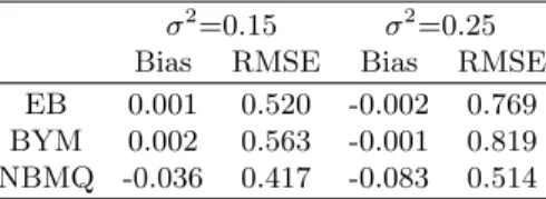
The mean values of Bias and RMSE over areas are set out in Table1. The bias results reported in Table 1 confirm our expectations: under both scenarios (σ2=0.15,0.25) the EB and the BYM perform better than the NBMQ predictors, whereas from the RMSE results we see that claims in the literature (Chambers and Tzavidis,2006) about the superior outlier robustness of M-quantile compared with the EB and BYM certainly hold true. A smearing-type estimator could reduce the bias of the NBMQ predictor. Note, however, that the cost of this bias-adjusted estimator is the inconsistency of (4.14), reflecting the usual bias-variance trade-off in outlier-robust estimation.
Table 1. Model-based simulation results: performances of predictors of relative risks for disease mapping
σ2=0.15 σ2=0.25 Bias RMSE Bias RMSE EB 0.001 0.520 -0.002 0.769 BYM 0.002 0.563 -0.001 0.819 NBMQ -0.036 0.417 -0.083 0.514
We now examine the performance of the nonparametric MSE estimator (4.15). Figure6shows the area-specific values of RMSE and average-estimated RMSE in case of σ2 = 0.15, 0.25. Estimator (4.15) performs well: it track the true RMSE, exhibiting a good stability and showing only a small amount of over-coverage.
Figure 5. Relative risks estimates using models: SMR, EB, BYM and NBMQ
7. Negative Binomial M-quantile Geographically Weighted regression
In environmental and epidemiological applications, observations that are spatially close may be more alike than observations that are further apart. One approach for incorporating spatial in-formation in a NBMQ regression model is to assume that the model coefficients themselves vary spatially across the geography of interest. Geographically Weighted Regression (GWR) (Fother-inghamand others,1997;Fotheringhamand others,2002;Yu and Wu,2004) models this spatial variation by using local rather than global parameters in the regression model. The GWR model
Figure 6. Area-specific values of RMSE (solid line) and average-estimated RMSE (dashed line) underσ2
equal to 0.15 (left) and 0.25 (right)
is a linear model for the conditional expectation ofygivenXat locationu. That is, a GWR model assumes spatial non-stationarity of the conditional mean of the variable of interest. In this Section we define a spatial extension to NBMQ regression based on Geographically Weighted regression by using the same approach bySalvatiand others(2012) for M-quantile GWR model. Givenn obser-vation at a set ofLlocations{ul;l= 1, . . . , L;L6n}, withnldata values{yil,xil;i= 1, . . . , nl}
observed at location ul, the NBMQGWR model can be defined by extending (4.10) to specify
a log-linear model for the M-quantile of orderq of the conditional distribution ofY givenXat locationu, writing
Qq(X;ψ, u) =texp(ηq(u)), (7.16)
whereηq(u) =Xβq(u), the linear predictor, varies withuas well as withq. The parameterβq(u)
can be estimated by solving the following estimating equations
Ψ(βq(u)) :=n−1 L X l=1 w(ul, u) nl X i=1 ψq(yi, Qq(xi;ψ, u)) =0, (7.17) where ψq(yi, Qq(xi;ψ, u) = n ψq(rilq)w(xil) Q0q(xil;ψ,u) V1/2(Q q(xil;ψ,u)) −a(βq(u)) o , w(ul, u) is a spatial
weighting function whose value depends on the distance from sample locationultouin the sense
that sample observations with locations close to ureceive more weight than those further away. In this paper we use a Gaussian specification for this weighting function
w(ul, u) = exp n
−d2u l,u/2b
2o, (7.18)
wheredul,udenotes the Euclidean distance betweenulanduandb >0 is the bandwidth. As the
distance between ul andu increases the spatial weight decreases exponentially. The bandwidth
b is a measure of how quickly the weighting function decays with increasing distance, and so determines the ‘roughness’ of the fitted GWR function. A spatial weighting function with a small bandwidth will typically result in a rougher fitted surface than the same function with
a large bandwidth. Spatial weights that vary with q can be defined by allowing the bandwidth underpinning these weights to vary withq. Such aq-specific optimal bandwidthbcan be obtained by minimising the following function with respect tob
L X l=1 nl X i=1 h yil−Qˆq(xil;ψ, uil, b) i2 , (7.19)
where ˆQq(xil;ψ, u, b) is the estimated value of the right hand side of (7.17) at quantileqand
lo-cationuil, using bandwidthbwhen the observationyilis omitted from the model fitting process.
However, using this q-specific cross-validation criterion can significantly increase the computa-tional time. For this reason, in this paper we use the optimal bandwidth atq= 0.5 for all other values ofqfor our extension of GWR to NBMQ regression. That is, the spatial weightsw(ul, u) in (7.17) do not depend on q. This is a reasonable first approximation to theq-specific optimal bandwidth that can be computed reasonably quickly, even if this choice could potentially lead to oversmoothing for small or large values of qand hence bias. The parameter θq(u) depends from
the location and can be estimated by solving
n−1 L X l=1 w(ul, u) nl X i=1 ψq2(rilq)−E ψ2q Y il−Qq(xil;ψ, u) V1/2(Q q(xil;ψ, u)) =0, (7.20)
where the expectationE[·] in (7.20) is a constant that ensures Fisher consistency for the estima-tion ofθq(u). The parameterθq(u) varies by locations and quantiles. To reduce the computational
time, an alternative approach is to use a value of globalθq(u) that varies by quantiles, but it is
fixed over space. For example, theθqestimated by equation (4.12). Given the spatial weights and
θq(u), the regression coefficients are estimated by the Fisher scoring for each locationu.
The M-quantile predictor of the rate in areaiis then ˆ
Qqil(xil;ψ, uil) =tilexp(x
T
iβˆqil(uil)), (7.21)
where fitted regression surface ˆQqil(xil;ψ, uil) = x
T
ilβˆq(uil) defines the fit of the NBMQGWR
model for the NB regression M-quantile of orderqilofyil givenxil at locationuil. Hereqilis the
M-quantile GWR coefficient for area iwith valuesyil andxil at location uil. It is calculated as
the unique valueqil such that ˆQqil(xil;ψ, uil)≈yil.
We have considered the Scottish real example dataset. For NBMQGWR we used informa-tions about centroids of each area under the Great Britain National Grid projection system. For BYMspatial model a BRugslibrary (a Rinterface to theOpenBUGSsoftware) has been used. For NBMQGWR we have used an originalRfunction available from the authors. Figure7shows the relative risk maps for both spatially structured models. Figure8 describes as using NBMQGWR the relative risks for some areas became more similar then obtained from BYMspatial: areas with higher relative risks considering spatial structure move on the diagonal.
8. Conclusion
In this paper, a class of robust Negative Binomial models and their extension to M-quantile approach have been proposed. The application to disease mapping of the M-quantile models is introduced and investigated. These models offer a natural way of modeling between area variabil-ity in data without imposing prior assumptions about the source of this variabilvariabil-ity. In particular, with M-quantile models there is no need to explicitly specify the random components of the
Figure 7. Relative risks estimates using models: NBMQGWR and BYMspatial
Figure 8. Relative risks estimates using different models: NBMQ, NBMQGWR and BYMspatial
model; rather, inter-area differences are captured via area-specific M-quantile coefficients. As a consequence, the M-quantile approach reduces the need for parametric assumptions. In addition, estimation and outlier robust inference under these models is straightforward. The proposed approach appears to be suitable for estimating a wide range of parameters and our simulation results show that it is a reasonable alternative to mixed effects models for ecological analysis on disease mapping.
Negative Binomial M-quantile Geographically Weighted Regression model. The choice of the model is crucial for the results of disease mapping. Further research seems to be necessary in order to develop tools for model selection of NBMQ based on robust quasi-deviance. Recently Machado and Santos Silva(2005) andLee and Neocleous(2010) have proposed quantile regression for count data and they overcome the problem with estimating conditional quantiles by adding to the count outcome noise generated from aU nif orm(0,1). This form of jittering creates artificial smoothness in the outcome and allows for modeling the continuos outcome by quantile regression because there is a one-to-one relationship between the conditional quantiles of the count outcome and those of the artificially generated continuos outcome. An alternative approach to modeling count data was proposed by Efron (1992) using asymmetric maximum likelihood estimation. Future research will be addressed to investigate these alternative methods and to compare these approach with the M-quantile method.
Appendix We have to evaluate: (i)E ψ Y i−µi V1/2(µ i) ; (ii)E ψ Y i−µi V1/2(µ i) Y i−µi V(µi) ; (iii)E ψ2 Y i−µi V1/2(µ i) ;
where Yi is distributed according to a NEGBIN2 distribution (seeCameron and Trivedi, 1998),
that is, P(Yi=yi) = Γ(yi+θ) Γ(θ)yi! µ i µi+θ yi θ µi+θ θ foryi= 0,1,2, . . .
Here,θis a positive integer,µi=E(Yi) andV(µi) = var(Yi) =µi+ µ2i
θ. SuchYican be regarded
as the number of failures for having θsuccesses in a sequence of Bernoulli trials. From now on, to make the notation easier, the indexi is suppressed. Accordingly, we writeµ instead ofµi, y
instead ofyi, and so on.
First, we evaluateE
Y I(Y ∈A)
andE
Y2I(Y ∈A)
, whereA={a, . . . , b−1}, 06a < b
are integers. LetA+ 1 ={a+ 1, . . . , b}. Then,
E
Y I(Y ∈A+ 1)
=E
Y I(Y ∈A)
−a P(Y =a) +b P(Y =b).
By the transformationz=y−1, one also obtains
EY I(Y ∈A+ 1) =P y∈A+1y Γ(y+θ) Γ(θ)y! µ µ+θ y θ µ+θ θ = µ+µθ P z∈A(z+θ) Γ(z+θ) Γ(θ)z! µ µ+θ z θ µ+θ θ = µ+µθ P z∈A(z+θ)P(Y =z) = µ+µθE Y I(Y ∈A) +µµ θ+θP(Y ∈A). Equating such expressions, one finally obtains
E[Y I(Y ∈A)] = µ+θ
θ [aP(Y =a)−bP(Y =b)] +µ P(Y ∈A). (8.22)
We next apply the same argument for calculatingE
Y2I(Y ∈A) . Then, E Y2I(Y ∈A+ 1) =E Y2I(Y ∈A) −a2P(Y =a) +b2P(Y =b) and EY2I(Y ∈A+ 1) =P y∈A+1y 2 Γ(y+θ) Γ(θ)y! µ µ+θ y θ µ+θ θ = µµ+θ P z∈A(z+ 1)(z+θ) Γ(z+θ) Γ(θ)z! µ µ+θ z θ µ+θ θ = µµ+θ P z∈A z 2+ (θ+ 1)z+θ P(Y =z) = µµ+θE Y2I(Y ∈A) +µµ(θ++1)θ E Y I(Y ∈A) +µµ θ+θP(Y ∈A). Again, equating the above expressions yields
EY2I(Y ∈A) = µ+θθ a2P(Y =a)−b2P(Y =b)+µ(θθ+1)E[Y I(Y ∈A)] +µ P(Y ∈A) = = µθ [θ+µθ+µ]P(Y ∈A) +µ+θθ a2P(Y =a)−b2P(Y =b) + +µ(µ+θθ)(2θ+1)[aP(Y =a)−bP(Y =b)] . (8.23)
Finally, the previous results, for a particular choice of Aallow to evaluate (i)-(ii)-(iii). Define ψ(r) = r −c6r6c c r > c −c r <−c and set r=VY1/−2(µµ).
Letj1 =bµ−c V1/2(µ)c andj2 =bµ+c V1/2(µ)c. Final results may change depending on whetherµ−c V1/2(µ) is integer or noninteger. In what follows, we consider the not integer case; the integer case can be handled similarly.
i) E ψ Y −µ V1/2(µ) =−c P Y −µ V1/2(µ) <−c +c P Y −µ V1/2(µ) > c + +E Y −µ V1/2(µ) I(−c6 Y −µ V1/2(µ) 6c) = Because VY1/−2(µµ) > c means Y > µ+c V
1/2(µ), as Y should be integer, we have Y
>
bµ+c V1/2(µ)c+ 1 =j2+ 1. Analogously, VY1/−2(µµ)<−c meansY < µ−c V
1/2(µ), which, whenµ−c V1/2(µ) is not integer leads toY 6bµ−c V1/2(µ)c=j1(whenµ−c V1/2(µ) is integer toY 6j1−1). Moreover,−c6 VY1/−2(µµ) 6cmeansµ−c V
1/2(µ)
6Y 6µ+c V1/2(µ)
which, whenµ−c V1/2(µ) is not integer isj
1+ 16Y 6j2 (whenµ−c V1/2(µ) is integer isj16Y 6j2). So, we obtain =−c P(Y 6j1) +c P(Y >j2+ 1) + + 1 V1/2(µ)E[Y I(j1+ 16Y 6j2)]− µ V1/2(µ)P(j1+ 16Y 6j2). ConsideringA={j1+ 1, . . . , j2} and also that
µ+θ θ (y+ 1)P(Y =y+ 1) = µ θyP(Y =y) +µP(Y =y) (8.24) we obtain E[Y I(j1+ 16Y 6j2)] =µP(j16Y 6j2−1)− µ θj2P(Y =j2) + µ θj1P(Y =j1) (8.25) and finally EhψVY1/−2(µµ) i =−c P(Y 6j1) +c P(Y >j2+ 1) + +V1/µ2(µ)P(Y =j1) 1 + j1 θ −V1/µ2(µ)P(Y =j2) 1 + j2 θ ii) E ψ Y −µ V1/2(µ) Y −µ V(µ) =− c V(µ)E[(Y −µ)I(Y 6j1)]+ c V(µ)E[(Y −µ)I(Y >j2+ 1)] + + 1 V3/2(µ)E (Y −µ)2I(j1+ 16Y 6j2) =
= µ c V(µ)P(Y 6j1) + µ c V(µ)P(Y 6j2) + µ2 V3/2(µ)P(j1+ 16Y 6j2) + − c V(µ)E[Y I(Y 6j1)]− c V(µ)E[Y I(Y 6j2)]− 2µ V3/2(µ)E[Y I(j1+ 16Y 6j2)] + + 1 V3/2(µ)E Y2I(j1+ 16Y 6j2) Considering result (8.25),A={0, . . . , j1}in (8.22) with (8.24)
E[Y I(Y 6j1)] =− µ θj1P(Y =j1) +µ P(Y 6j1−1), (8.26) and A={0, . . . , j2}in (8.22) with (8.24) E[Y I(Y 6j2)] =− µ θj2P(Y =j2) +µ P(Y 6j2−1) (8.27)
and againA={j1+ 1, . . . , j2}in (8.23) with (8.24)
E Y2I(j1+ 16Y 6j2)= µ θj 2 1P(Y =j1)− µ θj 2 2P(Y =j2) + (8.28) +µP(j16Y 6j2−1) + µ(θ+ 1) θ E[Y I(j16Y 6j2−1)] substituting (8.25,8.26,8.27, 8.28) E ψ Y −µ V1/2(µ) Y −µ V(µ) = µ c V(µ) P(Y =j1) j1+θ θ +P(Y =j2) j2+θ θ + + µ V3/2(µ) P(Y =j1) j1 θ (θ+ 1 +j1)−P(Y =j2) j2 θ (θ+ 1 +j2) +P(j16Y 6j2−1) + + µ 2 V3/2(µ) P(Y =j1) j 1−j1θ−θ2 θ2 −P(Y =j2) j 2−j2θ−θ2 θ2 +1 θP(j16Y 6j2−1) iii) E ψ2 Y −µ V1/2(µ) =c2[P(Y 6j1) +P(Y >j2+ 1)] + + 1 V(µ)E (Y −µ)2I(j1+ 16Y 6j2) = =c2[1−P(j1+ 16Y 6j2)] + µ2 V(µ)P(j1+ 16Y 6j2)+ − 2µ V(µ)E[Y I(j1+ 16Y 6j2)] + 1 V(µ)E[Y 2I(j 1+ 16Y 6j2)] = Substituting the values of the expected values (8.25,8.28) we arrive to
E ψ2 Y −µ V1/2(µ) =c2 [1−P(j1+ 16Y 6j2)]+ + µ V(µ) P(Y =j1) j1 θ (θ+ 1 +j1)−P(Y =j2) j2 θ (θ+ 1 +j2) +P(j16Y 6j2−1) + + µ 2 V(µ) P(Y =j1) j 1−j1θ−θ2 θ2 −P(Y =j2) j 2−j2θ−θ2 θ2 +1 θP(j16Y 6j2−1)
References
Assuncao, R.M. (2003). Space varying coefficient models for small area data. Environ-metrics 14, 453–473.
Besag, J., York, J.C. and Molli´e, A.(1991). Bayesian image restoration, with application
in spatial statistics (with discussion). Annals of the Institute of Statistical Mathematics 43, 1–59.
Breckling, J. and Chambers, R.(1988). M-quantiles. Biometrika 75, 761–771.
Breslow, N.E. (1984). Extra-poisson variation in log-linear models. Applied Statistics 33,
38–44.
Breslow, N.E. and Clayton, D.G.(1993). Approximate inference in generalized linear mixed models. Journal of the American Statistical Society 88, 9–25.
Cameron, A. C. and Trivedi, P. K.(1998). Regression Analysis of Count Data. Cambridge
University Press.
Cantoni, E. and Ronchetti, E. (2001). Robust inference for generalized linear models. Journal of the American Statistical Association 96, 1022–1030.
Chambers, R., Salvati, N. and Tzavidis, N.(2012). M-quantile regression models for binary
data in small area estimation. Submitted: available from the authors upon request.
Chambers, R. and Tzavidis, N. (2006). M-quantile models for small area estimation. Biometrika 93, 255–268.
Clayton, D. and Kaldor, J. (1987). Empirical bayes estimates of age-standardized relative risks for use in disease mapping. Biometrics 43, 671––681.
Efron, B. (1992). Poisson overdispersion estimates based on the method of asymmetric
maxi-mum likelihood. Journal of the American Statistical Association 87, 98–107.
Efron, B. and Morris, C.(1973). Stein’s estimation rule and its competitors - an empirical
bayes approach. Journal of the American Statistical Association68, 117–130.
Fotheringham, A.S., Brundson, C. and Charlton, M.(1997). Two techniques for
explor-ing non-stationarity in geographical data. Journal of Geographical Systems 4, 59–82.
Fotheringham, A.S., Brundson, C. and Charlton, M. (2002). Geographically Weighted Regression. West Sussex: John Wiley & Sons.
Ghosh, M. (1992). Constrained bayes estimation with applications. Journal of the American Statistical Association 87, 533–540.
Green, P.J. and Richardson, S.(2002). Hidden markov models and disease mapping.Journal of the Statistical Association 97, 1–16.
He, X.(1997). Quantile curves without crossing. American Statisticians 51, 186–192. Huber, P.J.(1981). Robust Statistics. London: Wiley.
Kensall, J.E. and Wakefield, J.C. (1999). Discussion of “Bayesian Models for Spatially Correlated Disease and Exposure Data”, Bayesian Statistics 6 edition. Ney York Oxford Uni-versity Press.
Kokic, P., Chambers, R., Breckling, J. and Beare, S. (1997). A measure of production performance. Journal of Business and Economic Statistics 10, 419–435.
Lawless, J.F.(1987). Negative binomial and mixed poisson regression. The Canadian Journal of Statistics 15, 209–225.
Lee, D. and Neocleous, T. (2010). Bayesian quantile regression for count data with
appli-cation to environmental epidemiology. Journal of the Royal Statistical Society Series C 59, 905–920.
Louis, T.A.(1984). Estimating a population of parameter values using empirical bayes methods. Journal of the American Statistical Association 79, 393–398.
Machado, J.A.F. and Santos Silva, J. M. C.(2005). Quantiles for counts. Journal of the American Statistical Association 100, 1226–1237.
MacNab, Y.C. (2009). Bayesian multivariate disease mapping and ecological regression with errors in covariates: Bayesian estimation of dalys and ‘preventable’ dalys. Statistics in Medicine 28, 1369–1385.
MacNab, Y.C.(2010). On bayesian shared component disease mapping and ecological regression
with errors in covariates. Statistics in Medicine 29, 1239–1249.
McCullagh, P. and Nelder, J.A.(1989).Generalized Linear Models, second edition edition.
London – New York: Chapman and Hall.
Pratesi, M., Ranalli, M.G. and Salvati, N.(2009). Semiparametric m-quantile regression
using penalized splines. Journal of Nonparametric Statistics 21, 287–304.
Rao, J.N.K.(2003). Small Area estimation. Wiley Series in Survey methodology.
Salvati, N., Tzavidis, N., Pratesi, M. and Chambers, R. (2012). Small area estimation via m-quantile geographically weighted regression. Test 21, 1–28.
Wakefield, J.(2007). Disease mapping and spatial regression with count data. Biostatistics8, 158–183.
Yu, D.L. and Wu, C. (2004). Understanding population segregation from landsat
etm+imagery: a geographically weighted regression approach. GISience and Remote Sens-ing 41, 145–164.