Magnetic Resonance Images.
Niels Vver Hartvig
University of Aarhus
Revised version
March 9th2001
Abstract
In functionalmagnetic resonance imaging,spatialactivation patterns are
com-monly estimated using a non-parametric smoothing approach. Signicant peaks
or clusters in the smoothed image are subsequently identied by testing the null
hypothesisoflackofactivationineveryvolumeelementofthescans. Aweaknessof
thisapproachisthelackofamodelfortheactivationpattern;thismakesitdiÆcult
todeterminethevarianceofestimates,totestspecicneuroscientichypothesesor
to incorporate priorinformationaboutthebrainareaunder studyintheanalysis.
Theseissues maybeaddressed byformulating explicitspatialmodelsforthe
acti-vationand usingsimulationmethodsforinference. Wepresent one suchapproach,
basedon a marked point process prior. Informally,one maythinkof thepointsas
centresofactivation,andthemarksasparametersdescribingtheshapeandareaof
thesurrounding cluster. We present an MCMCalgorithm formaking inference in
the model, and compare the approach with a traditional non-parametric method,
usingboth simulatedand visualstimulation data. Finallywe discussrelevant
ex-tensionsof themodeland the inferential framework to account for non-stationary
responsesand spatio-temporal correlation.
Keywords: Functional magnetic resonance imaging;Stochastic geometry model; Marked
point process; Markov chain Monte Carlo;State space model.
1 Introduction
Functional magnetic resonance imaging(fMRI) uses the dierent magnetic properties of
oxy- and deoxyhaemoglobin to visualize localized changes in blood ow, blood volume
and blood oxygenation in the brain. These are in turn indicators for local changes in
Department of Mathematical Sciences, Universityof Aarhus, Ny Munkegade, DK-8000Aarhus C,
neuralactivity. By exposing asubject tocontrolledstimuli,which are carefullydesigned
toaectonlycertainbrainfunctions,itispossible toestimatethe anatomicallocationof
neuronesinvolvedinthecorrespondingfunctions. Brainfunctionmaythenbemappedto
brainanatomybycombiningfMRIscanswithanatomicalscansobtainedbyconventional
MRI.
The technique is quite new; one of the rst experiments was reported by Kwong
et al.(1992), andsince then the numberof publicationsinthe eld has grown extremely
fast. Today fMRI is one of the most important modalities for imaging the brain, since
it is completely non-invasive, has a reasonable temporal resolution (about 2 sec) and
an excellent spatial resolution (about 2 mm). See Lange (1996) or Hartvig (2000) for
introductions to the subject.
The data obtained in anfMRI experiment isa time series ofthree dimensional scans
of the brain, as well as covariates describing the presentation of stimuli. In the analysis
ofthe data,the signalofinterestis aspatio-temporalprocess, wherethetemporalprole
is coupled to the stimulation rhythm through the haemodynamic response to neural
activation(also knownastheBOLDeect). Theresponselagsthe neuralactivationwith
about 6 sec., and ismore smooth than the latter. Empirically, the impulse response has
been found to look roughly like a Gamma density, but despite attempts to explain this
quantitatively (Buxton et al., 1998), there is still not a fully accepted biological model
for the process.
Generallytheneuronesinvolvedinaspecictaskareexpectedtopossesspatial
struc-ture, yielding a spatially correlated neural activation process. The resulting
haemody-namic oxygenation changes contribute further to this correlation, as they diuse in the
venoussideofthecapillarysystem,spreadingoverseveralmillimetres. Modellingthe
spa-tialstructureof thishaemodynamicprocessis adiÆculttask: Firstlythe overallpattern
willofcoursedependonthe typeof stimulation,anditisdiÆculttoimpose structureon
this ina generalsetting. Secondly the complexgeometry of the corticalsurface makesit
diÆculttodene relevant neighbourhoodsinthe space of volume elements(orvoxels)of
the scanned brain.
Instead, a common approach is to estimate the activation magnitude separately in
each voxel by a one dimensional time series model, see for instance Worsley and Friston
(1995), Lange and Zeger (1997), Bullmore et al. (1996)or Genovese (2000). The spatial
structureofthedataisincludedinasecondstep,whentheimage(orvolume)ofmarginal
estimates is convolved with a smoothing kernel, to obtain a non-parametric spatial
esti-mate. Subsequently, signicant peaks or clusters in the image are identied, by testing
the nullhypothesisof lackof activationateachvoxel,and the nal estimatemay consist
of voxels that are signicantly higherthan what would be expected by chance. Here the
signicance levelis corrected forthe large numberof hypotheses tested, usingresults for
Gaussianrandom elds (Worsley, 1995).
The fundamental problemin this approach is the lack of a model for the activation,
i.e.thereisnomodelforthedistributionofthestatisticsunderthe alternativehypothesis
that avoxel is active,and noassumptions are made about the distribution ofshape and
In this paper we propose a spatial model, by which some of these problems may
be addressed. The model is motivated by two fundamental assumptions in the fMRI
literature,whichare basedpartlyonthe spatialstructureonaneuronal level,and partly
on the haemodynamic origin of the signal: 1) The activated areas have a spatial extent
of several millimetres and 2) the activation pattern is \smooth". Using these, we will
modelthe activation surface as acollectionof Gaussian functions,which tosome extent
represent individual centres in the brain. This is formulated as a stochastic geometry
model based on marked point process prior (Baddeley and van Lieshout, 1993), where
the points stand for the locations and the marks describe the shape and height of the
centres. The inference in the model is based onsimulationtechniques, by whichwe can
estimatetheposteriormeanof functionsofinterest,suchasthe meanactivationpattern.
One advantage, compared to the typical analysis outlined above, is a more precise
estimateof thespatialpattern. Thismaybeparticularlyrelevantforshorttimeseries,in
experiments withmany dierenttypesof stimuliorinsituationswheresignal estimation
is more important than just signal detection. The latter is the case for instance in
pre-surgical planning or when fMRI is combined with other imaging modalities. A further
motivationisthe extended inferential scope, which allows ustoassess the uncertainty of
estimatesinaBayesianframework,ortoquantifythebeliefinmorespecichypothesesby
estimating posterior probabilities. Finally the haemodynamicresponse functionmay be
modelledinasemi-parametricway,whichallowsfornon-stationaritiesandnon-linearities.
Withthe latterapproachexplicitknowledge ofthe stimulationparadigmisnot required,
andwecanhenceestimateactivationwhichisnottime-lockedtothestimulationrhythm.
The paper is organized as follows: We rst present a typical set of fMRI data and
its preprocessing inSection 2. In Section 3 we formulate the basic modelfor the spatial
activation pattern and combine this with a simple model for the temporal response to
obtain a spatio-temporalmodel. The temporalpatternis assumed tobeknown and
de-scribedby aconvolutionmodel. Theposteriorinferenceisdoneby anMCMC algorithm,
which is described in Section 4. In Section 5 we apply the model to simulated data,
whichisusedforestimating priorparameters,and tovisualstimulationdata. Finallywe
discussrelevantextensions inSection6,toaccountforcorrelated noiseornon-stationary
responses, and give a conclusion inSection7.
2 fMRI data and its preprocessing
For illustration, we will consider data acquired in a well studied experimental design,
namely avisualstimulationpresented periodicallyin blocks of20 seconds. The stimulus
was alight,ashedwith 7 Hz infrontof the right eye of the subject. 90so-called
Echo-Planar Imaging scans were acquired during a 3 minute period, with an inter-scan time
(or repetition time) of 2 seconds. The stimulation was arranged inblocks of 20 seconds
o, 20 seconds on, 20 seconds o etc., with 4 complete on-o cycles during the session.
Eachvolume ofscansconsistsof5slicesof thickness 5mm,eachcomprisedof 128by 128
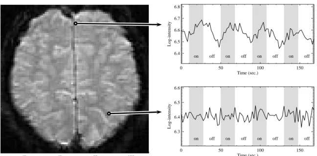
Figure 1 is a graphical illustration of the data. The left panel displays a section
of a slice from one of the scans, oriented in an oblique axial-coronaldirection with the
posteriorpartofthebraininthetopoftheimage. Therightpanelsdisplaytwovoxeltime
series; one is located inthe visual cortex, which is known to process visual impressions,
the other is located in an area where activation is not expected. The uctuation in the
former series is evident, as isthe haemodynamicdelay and dispersement.
40
60
80
100
40
60
80
100
on
off
on
off
on
off
on
off
0
50
100
150
Time (sec.)
6.3
6.4
6.5
6.6
Log-intensity
on
off
on
off
on
off
on
off
0
50
100
150
Time (sec.)
6.4
6.5
6.6
6.7
6.8
Log-intensity
Figure 1: Graphical illustration of visual stimulation fMRI data. Left: A section of an MR
scan of a slice of the brain. Right: Time series of respectively an active (top) and non-active
(bottom)voxel. Thestimulationepochsareindicatedby greybars.
The scans are almost always preprocessed before the statistical analysis to reduce
artifacts caused by the scanner or by subject movement, or to map individual brains to
a standard atlas. To correct for movement artifacts, we have used a simple procedure,
where each image is aligned to a reference image by minimizing the squared dierence
between the two images over all translations and rotations. Often dierent types of
trends and low-frequency uctuations may be observed in the voxel time series. These
may be caused by scanner instability, by physiological processes or by aliased cardiac
and respiratory pulsations. We chose a very simple correction for this, by subtracting
a tted linear trend term in each voxel time series. More general trend and uctuation
models, such asacosinebasis proposedbyHolmes et al.(1997),may beapplied. As will
be clear later,however, our focus ispartly to modelgeneraltemporalresponse patterns,
and hence we are cautiousnot to remove any uctuations related tothe haemodynamic
response. A linear term isa good compromisein this context.
Finally we log-transformed the data to stabilize variances. Furthermore, this
trans-formation is motivated by the fact that the units of the MR scanner are arbitrary and
log-the original series.
Let Y =fY
it
;i2V;t=1;:::;mg denote the preprocessed fMRI time series. Here V
is the set of voxels covering brain tissue, V S, where S represents a two dimensional
slice or a three dimensionalvolume of the brain, and m is the number of scans. We will
let
t
denotethe stimulationfunction, where
t
=1indicates stimulationand
t
=0no
stimulationat time t.
3 The model
Our general model has the form
Y it =(A i (X)+ i )' t +" it ; where = f i ;i 2 Vg and " = f" it
;i 2 V;t = 1;:::;mg are Gaussian processes. Here
A(X) = fA
i
(X);i 2 Vg is the magnitude of activation, which is parametrized by a
marked pointprocess X,and '=f'
t
;t =1;:::;mg is the temporalvariationcausedby
the BOLD eect. We will describe in detail how the spatial and temporalpatterns are
modelled inthe following.
3.1 A model for the spatial activation pattern
Consider rst the case where data only represent a two dimensional slice of the brain,
that is V S R 2
. We will describe the spatial activation pattern by a marked point
process X =fX 1 ;X 2 ;:::;X n g, where X k = ( k ;a k ;d k ;r k ; k ). A point X k may to some
extent be considered as a centre of activation with location
k
2 S, and where the four
marks (a k ;d k ;r k ; k
) describe the magnitude and shape of the centre. The activation
pattern fA
i (X)g
i2V
is assumed to have a specic geometry, namely a sum of Gaussian
functions, A i (X)= P n k=1 h(i;X k ); where h(i;X k )=a k exp log2 d k j 2 1 r k =(1 r k ) + j 2 2 (1 r k )=r k ; (1) here (j 1 ;j 2 )=R ( k )(i k
)and R () isarotationwith angle. This representation is
motivatedbythecommonassumptionsofsmoothnessandspatialextentoftheactivation,
andtheheuristicideaisthatageneralsmoothactivationsurfacewithfewlocalizedpeaks,
may be well approximated by a collectionof Gaussian functions. The interpretation of
theparametersisthata
k 2R
+
istheheightoftheGaussianbellatthecentre
k ,d
k 2R
+
isthe areaofthe contourellipseathalfheight,r
k
2(0;1)isameasure ofthe eccentricity
of the ellipse, more precisely the ratio of the rst principal axis and the sum of the two
axes, and
k
2[ =4;=4] is the orientationof the ellipse.
We have specic prior knowledgeon the parameters of the model. The magnitude is
typicallyabout2%-5%ofthe baselineintensity,weexpect theactivationclusterstocover
function under study. Furthermore a typical point conguration should contain only a
moderatenumberofpoints. ThismaybeincludedinthemodelinaBayesianframework,
and we will therefore consider the process X as a realization of a randomvariable with
a prior distribution. Each centre X k is a point in X = S M, where M = [0;C a ][0;C d ] (0;1) [ =4;=4]: Here C a and C d
are natural bounds for the height and area, respectively.
Let X be equipped with the Borel -eld S M and the Lebesque measure
2
4 ,
and let denote the exponential space over X, that is the set of nite sets fx
1 ;:::;x n g where x i
2 X for all i. The process X is then a point process in or, equivalently, a
marked point process with point space S and mark space M. We will assume that the
prior distribution has density
p(x)/ n Y k=1 (( k )p(a k )p(d k )p(r k )); x2; (2)
withrespecttotheunitratePoissonprocesson, wheren=n(x)isthenumberofpoints
in x. Here () is an intensity function, which may give preference to specic cortical
areas, ormay be constantif there is noprior knowledge of where the activation islikely
to occur, and p() is a generic notation for prior densities of the three mark parameters
a k , d k and r k .
3.1.1 Priors for the marks
Thepriorsforaanddshouldbeasuniformaspossible,yetpenalizingvaluesclosetozero.
The inverse Gamma distribution is a suitable choice in this context, with its light tail
near zeroand quiteheavy tailforlarge values. Hencewe willassume thata 1 (2; a ) and d 1 (2; d
) with the restrictions that a 2 (0;C
a ] and d2 (0;C d ]. The density of d is p(d)=exp ( d =C d )( d =C d +1) 1 2 d d 3 exp ( d =d); d2(0;C d ]: Theupper-boundsC a andC d
arenaturalboundsforthemagnitudeandsizeofactivation
clusters. The priormean of d is
d =(1+ d =C d ),or approximately d whenC d is large.
As for the axis ratio r we wish to discourage very eccentric ellipses. This can be
obtained by aBeta-prior, rBeta(
r ;
r ):
3.1.2 The intensity function
The intensity function provides a exible tool for incorporating substantial prior
infor-mation onthe position of the activation. One possibility is touse anatomical covariates
obtainedfromahigh-resolutionscanofthe brain,acquiredsimultaneouslywiththe
func-tionalscans. Arelevantanatomicalconstraintistorestrictactivationtothe graymatter
sheet of the cortical surface (Kiebelet al., 2000). A simple approach toaddressing this,
is to segment the high-resolution scan, and let the intensity function favour points
lo-catedingray matter. Usingasoft constraintlikethisallowsfor somedegree ofvariation
Another interesting possibilityis touse functionalprior information,forinstance
ob-tainedfrom aprevious experimenton the samesubject. This ts wellwith the Bayesian
paradigmof sequential updatingof information,and may improve eÆciency in the
anal-ysis by eectively restricting focus to relevant areas, yet allowing for variations from
one experiment to the other. Since the activation pattern may be quite variable even
in replicated experiments, also in this case a soft constraint in a Bayesian framework is
appropriate.
3.2 A model for the temporal pattern
Thesimplest modelforthe temporalpattern'isaxed regression model. The response
is to a good approximation time-invariant and additive (Boynton et al., 1996), which
leads to a convolution model, where an impulse response function is convolved with
the stimulation function to obtain '. Based on empirical studies, Friston et al. (1995)
suggested to use a Gaussian density with mean 6 sec. and variance 9 sec. 2
as impulse
response, to model the delay and dispersion of the haemodynamic response. We will
adopt this choice here, and thus let
' t = X i t i T p 23 exp ( (iT 6) 2 18 ); (3)
where T is the repetition time. This simplicity of this model makes it an attractive
starting point, as it allows us to focus on the spatial pattern in the inference, which
simpliesthe simulationprocedure signicantly.
The basic assumption made here, is that the spatio-temporal activation prole is
separable, i.e. that the response function isthe same inall voxels. We willdiscuss later,
how the model may be extended to relax this assumption, and to account for a
non-stationary response that changesover time.
3.3 Combining the spatial and temporal models
Given the centres X and the haemodynamic response function ', the model for the
intensity Y is, Y it =(A i (X)+ i )' t +" it ; (4) where =f i ;i 2 Vg N(0; 2 I jVj ), " =f" it ;i 2 V;t =1;:::;mg N(0; 2 I jVj I m )
and and " are independent. The likelihoodfunction is given by
p(Yjx)=(2 2 ) (m 1)jVj 2 exp ( 1 2 2 X i2V m X t=1 Y it ~ Y i ' t 2 ) (2( 2 + 2 ss ' )) V 2 exp ( 1 2( 2 =ss ' + 2 ) X ~ Y i A i (x) 2 ) : (5)
Here ~
Y
i
is the coeÆcient of the projection of fY
it
;t = 1;:::;mg on the vector space
L=spanf'g, ~ Y i = m X t=1 Y it ' t =ss ' ; ss ' = m X t=1 ' 2 t : (6)
Notice that the likelihood function factorizes intotwo terms, involvingonly the
pro-jection ofY ontoL andonto the orthogonalcomplement toL,respectively, with X only
entering in the former. Hence we nd that the regression image f ~
Y
i
;i 2 Vg, which is
known as a Statistical Parametric Map (SPM) in the brain imaging literature (Friston
et al.,1994),issuÆcientforX. Asmentionedearlier,usually theSPM issmoothedwith
aGaussiankernel toobtainanon-parametric estimateofthe activation,and the present
setup may thus be viewed as analternativeanalysis of the SPM, based ona parametric
model.
The purpose of the random eect term
i
is to regularize the estimate of X. To see
whythisisnecessary,considerthelogposteriordistributionofX,whichuptoanadditive
constant is given by logp(xjY)= 1 2( 2 =ss ' + 2 ) X i2V ~ Y i A i (x) 2 +logp(x):
Suppose for amomentthat =0,correspondingtoomittingthe randomeect
i
above.
ByinsertingsuÆcientlymanysmallbells,wecanobtainacongurationwhereA
i (x)=
~
Y
i
when the latter is positive, and A
i
(x) = 0 elsewhere. This will minimize the sum of
squaresabove. Even ifthe priordensityof suchapathologicalpointcongurationisvery
small, it will be the maximum a posteriori estimate in the limit as m, and hence ss
' ,
tendstoinnity,sincethesum ofsquareswilldominateinthe limit. Byassumingaxed
positive value for 2
this undesirable property of the posterior distribution is removed.
Intuitively 2
is a measure of how well we expect the actual activation surface to be
described by areasonable collectionofGaussianfunctions,whilethe purpose ofthe prior
for X isto quantify what we mean by a reasonable collection.
Wewillusesimpleestimates forthevarianceparameters. Anunbiasedandconsistent
estimatorfor 2 isgiven by ^ 2 = 1 (m 1)jVj X i2V m X t=1 Y it ~ Y i ' t 2 2 2 (f)=f; f =(m 1)jVj: (7) Asfor 2 ,wewillestimate 2 =ss ' + 2
byconsideringtheregressioncoeÆcients ~
Y
i
. These
are mutuallyindependent and distributed as
~ Y i N(A i (x); 2 =ss ' + 2 ); i2V:
Letting @i denotethe 9-voxel neighbourhoodof i, we willlet
Y i = 1 9 X ~ Y j N( A i (x); 1 9 ( 2 =ss ' + 2 ))
for i2V Æ
, where V Æ
=fi2V j@iVg. By assumingthat the activation surface A
i (x)
can be approximated by aplane locallyaround i,we havethat A
i (x)= A i (x)and hence that 9 8jV Æ j X i2V Æ ~ Y i Y i 2 (8)
is anunbiased and consistentestimator for 2
=ss
' +
2
. When the approximation is not
exact, we willget aslight positive bias inthe estimate for 2
.
4 Simulating from the posterior distribution
In ordertoexplore the posteriordistribution ofthe activationcentres given the data, we
have designed a Metropolis-Hastings algorithm based on the Geyer and Mller (1994)
algorithm for general nite point processes. This algorithm is a special case of the
reversible-jump algorithmof Green (1995), where the Jacobianterm is always one. Let
x be the current point conguration. We will then propose to 1) insert a new point, 2)
remove an existing point or3) change anexisting point,with probabilities p
1 , p 2 and p 3 respectively, wherep 1 +p 2 +p 3
=1. By\changean existingpoint"wemean that one of
the coordinates of the point ischanged, either the position orone of the marks.
Let q
m (x
0
jx) denote the proposal density of a new conguration x 0
based on the
current conguration x with move type m = 1;2;3. The probability of accepting the
moveis then respectively
1 (x;x 0 )=min p(x 0 jY)q 2 (xjx 0 )p 2 p(xjY)q 1 (x 0 jx)p 1 ;1 ; 2 (x;x 0 )=min p(x 0 jY)q 1 (xjx 0 )p 1 p(xjY)q 2 (x 0 jx)p 2 ;1 ; 3 (x;x 0 )=min p(x 0 jY)q 3 (xjx 0 ) p(xjY)q 3 (x 0 jx) ;1 :
If the move is rejected, the Markov chain stays in x. The proposal distributions are
described indetail inthe following.
4.1 Insertion of a point
Withprobabilityp
1
we propose toadda newpoint =(;a;d;r;)tothe existingpoint
conguration x= fx
1 ;:::;x
n
g. In order to obtain a reasonable acceptance rate for this
move,wewishtoperformaGibbs-likeupdateand samplethe parametersfromadensity
proportionaltotheconditionalintensityp(x[jY)=p(xjY). Howeverthisisadistribution
onthesixdimensionalspaceofpointsandmarksanditisnotpossibletosimulatedirectly
from it. Instead, we will propose the parameters (;a;d;r;) sequentially, suchthat the
proposalq
1
(x[jx) isa combinationof the terms
where we use the generic symbol q(j) for a proposal density. We will choose the
pro-posal of a single parameter, a say, such that it resembles the conditional intensity of a
point(;a;d 0 ;r 0 ; 0
)giventhe currentcongurationx,where(d
0 ;r
0 ;
0
)arexed typical
values for the remaining parameters and is the proposed position of the point. In our
applications we have chosen a
0
= 0:01, d
0
= 50 mm 2
(corresponding to about 14 voxels
inour data),r
0
=0:5and
0
=0. Generallywesimulatefromdiscretizedapproximations
tothe conditionalintensities,the details are given below.
Using (5) we nd that when ignoring the priors, the conditional intensity of a new
point given x is p(Yjx[) p(Yjx) =exp ( 1 2( 2 =ss ' + 2 ) X i2V h(i;) 2 2 X i2V h(i;)( ~ Y i A i (x)) !) : (10)
By approximating the discretesum by anintegral, we nd
X i2V h(i;) 2 ' ZZ a 2 exp 2log2 d x 2 r=(1 r) + y 2 (1 r)=r dxdy=(v x v y ) = ZZ a 2 exp 2log2 d (x 2 +y 2 ) dxdy=(v x v y ) =a 2 d=(2log2v x v y )=a 2 ~ d=(2log2); (11) where v x and v y
are the length of the voxel sides in mm and ~ d = d=(v x v y ) is the area
measured in voxels. Above (x
;y
) represents a translation and rotation of (x;y), and
thesecondequalityfollowssincethis transformationtogether withthe coordinatescaling
has Jacobian one.
When proposing the positionwe willx theremainingparameters at(a
0 ;d 0 ;r 0 ; 0 )
and approximate the intensity in(10) with a voxel-wise constant density;
q(jx)/exp ( 1 ( 2 =ss ' + 2 ) X i2V h(i;;a 0 ;d 0 ;r 0 ; 0 )( ~ Y i A i (x)) ) for 2V:
The log-proposalis thus proportional to the convolution of the residual image with the
typical activation centre, which may be calculated eÆciently in the Fourier domain, see
Press et al. (1992). Considering (10) as a function of the height a, the proposaldensity
is q(aj;x) /exp ( 1 2( 2 =ss ' + 2 ) a 2 d 0 2log2v x v y 2a X i2V h(i;;1;d 0 ;r 0 ; 0 )( ~ Y i A i (x)) !) ; (12)
whichis aGaussian distribution,
aj;xN P i2V h(i;;1;d 0 ;r 0 ; 0 )( ~ Y i A i (x)) ~ d =(2log2) ; 2 =ss ' + 2 ~ d =(2log2) ! ;
restricted to the interval(0;C
a
]. As for the three remaining parameters (d;r;) we will
approximate the conditional intensity with a piecewise log-linear intensity, and sample
fromthe corresponding distribution. When proposing d wewillselect agrid (Æ
0 ;:::;Æ m ) such that Æ 0 =0, Æ m =C d and let q(dj;a;x)/exp p i 1 + p i p i 1 Æ i Æ i 1 (d Æ i 1 ) for d2(Æ i 1 ;Æ i ]; where p i = 1 2( 2 =ss ' + 2 ) Æ i a 2 2log2v x v y 2 X i2V h(i;;a;Æ i ;r 0 ; 0 )( ~ Y i A i (x)) ! 3logÆ i d =Æ i ; (13) for i = 1;:::;m 1, p 0 = p 1 and p m =p m 1
. Above the last two terms stem from the
prior for d. The expressions for q(rj;a;d;x)and q(j;a;d;r;x)are derived similarly.
4.2 Removal of a point
With probability p
2
we propose to remove a point. If the current conguration x is
empty we donothing,otherwise weselect the candidatefrom the pointsin xwith equal
probability 1=n(x).
4.3 Moving a point
Withprobabilityp
3
wepropose tochange aparameter ofa randomlyselected point. We
choose one of the parameters , a, d, r or with equal probability and a new value is
proposed by considering the conditional distribution given the other parameters.
Suppose forinstance that apoint=(;a;d;r;)2xhas beenselected and we wish
topropose anew position 0
for. Corresponding tothe insertionof anew pointabove,
we willthen propose thepositionby simulatingfroma distributionwhichhas voxel-wise
constant density q( 0 jx)/exp ( 1 ( 2 =ss ' + 2 ) X i2V h(i; 0 ;a;d;r;)( ~ Y i A i (xn)) ) ; 0 2V:
For the parametersr,d and we consider aneighbourhoodof the currentvalue, and
approximate the conditionaldensity asin(13) above. In ourapplication,we have chosen
a neighbourhood of 100 mm 2
for d, 0.3 for r and 0.35 for .
Finally,theheighta issimulatedfromanormaldistributionaswhenproposinganew
point, ajxN P i2V h(i;;1;d;r;)( ~ Y i A i (xn)) ~ d=(2log2) ; 2 =ss ' + 2 ~ d=(2log2) ! :
5 Applications
5.1 A simulation study
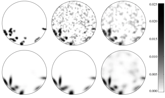
We simulated data from the model(4) with a known activation pattern A, displayed in
Figure2. Thepatternmimicsa\true"activationimage,inthesense thatithascoherent
regions of activation of both small and moderate size, and by the fact that it is more
complex than any single realization of the stochastic geometry model.
Weperformedaninformalsensitivityanalysis, wheredierentparametersof theprior
were studied. We used three dierentvalues of a constant intensity ()= (0.01, 0.1,
1.0) and two dierent values of respectively
a (0.02, 0.05) and d (50 mm 2 , 200 mm 2 ) (assuming a voxel-size of 3.52 mm 2
as for the real data.) For all runs, we set
r = 5.
Foreachparametercombination,weobtained 600000iterationsofthe MCMC algorithm
as described in the previous section, where ateach step one of the points were updated,
or a change inthe number of pointswas proposed. By diagnostic plots, the chains were
judged to be stationary after a burn-in of 100000 iterations, and we subsampled every
100'th iterationfromthis pointto obtain 5000samples.
0.000
0.005
0.010
0.015
0.020
0.025
Figure 2: Top row: True activation pattern (left) and non-parametric estimates with
kernel-width 2 voxels (middle) and 3 voxels (right). Bottom row: Estimates of posterior mean
acti-vation from the model. Left: =0:1,
d =200 mm 2 , a =0:05, middle: =0:01, d =200 mm 2 , a =0:05, right: =1:0, d =50 mm 2 , a
=0:02. For displaypurposes,theintensities
Figure2showsusualnon-parametricestimates, obtainedby smoothingthe regression
image f ~
Y
i
g with a Gaussian kernel of full-width-at-half-maximum (FWHM) 2 and 3
voxels respectively. These are typical choices of the kernel-width in the neuroimaging
literature; often a width of 3 voxels is used to ensure that the estimate is suÆciently
smooth to approximate a continuous random eld. The gure displays three posterior
mean activation estimates as well, where the eect of the prior parameters is evident:
When restricting the number of points by reducing (middle panel), the two regions
in the lower left part of the image, is merged to one. On the other hand, when the
insertionofnewbellsisencouraged,byincreasingandreducing
d and
a
(rightpanel),
the activation pattern is sensitive to noise, and is more similar to the non-parametric
estimates. The parameter setting of the left-most panel isthe best compromise between
robustness and sensitivity in this case, as measured by the posterior mean L 2
-distance
between the model activation pattern and the true pattern (Table 1). As a typical
summarystatisticofinterest,wealsoconsiderthe posteriormeanandstandarddeviation
of the integrated activation, i.e. the integral of the activation surface. The true value
is 3.49, which is within one standard deviation from the mean for the rst parameter
combination.
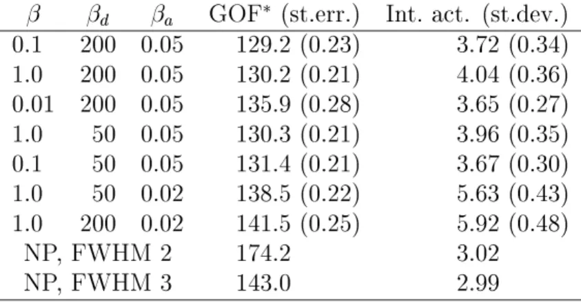
Table 1: Goodness-of-t (GOF) of the model with dierent parameter values. The mean
L 2
-distance between the model activation and the true pattern is used as a goodness-of-t
measure. Standarderrors dueto simulationaregiven inparentheses. Thelastcolumncontains
theposteriormeanandstandarddeviationoftheintegratedactivation,i.e.thetotalmassunder
the activation surface. The true value is 3.49. The two last linesdisplaycorresponding values
forthenon-parametric estimates.
d a GOF
(st.err.) Int.act. (st.dev.)
0.1 200 0.05 129.2 (0.23) 3.72 (0.34) 1.0 200 0.05 130.2 (0.21) 4.04 (0.36) 0.01 200 0.05 135.9 (0.28) 3.65 (0.27) 1.0 50 0.05 130.3 (0.21) 3.96 (0.35) 0.1 50 0.05 131.4 (0.21) 3.67 (0.30) 1.0 50 0.02 138.5 (0.22) 5.63 (0.43) 1.0 200 0.02 141.5 (0.25) 5.92 (0.48) NP, FWHM 2 174.2 3.02 NP, FWHM 3 143.0 2.99 Scaledby10 3
As it is often the case in Bayesian image analysis, we have no rigorous method for
selectingthe parametersof the prior. Asimpleapproach istouse simulationstudies like
this, to determine sensible combinations. Furthermore, the parameters
a
and
d are
directly relatedto the size and magnitude of activation clusters, hence sensible values of
these may be determined fromprevious experience.
estimate. We may, however, still perform an isolated comparison of estimates obtained
by the two procedures, both visually inFigure 2and by the summaryvalues inTable 1.
In both casesthe model-based estimateseemstobe muchmore precisethanthe FWHM
2 estimate, and slightly better than the FWHM 3 estimate. An argument against this
comparison, however, is the fact that the non-parametric images are often thresholded,
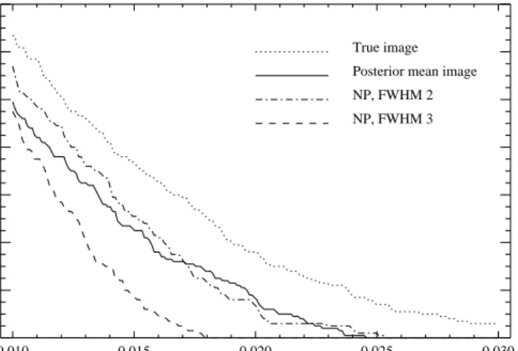
and only the set of supra-threshold voxels isused asan activation estimate. The plot of
the number of supra-threshold voxels as a function of threshold level inFigure 3 allows
for a comparison of the estimates from this point of view. Here there is only a slight
dierence between the FWHM 2 estimate and the model-based one. The FWHM 3
estimate, however, tends to oversmooth the activation patternmuch more than the two
others.
0.010
0.015
0.020
0.025
0.030
Threshold level
0
20
40
60
80
100
120
140
No. of voxels above threshold
True image
Posterior mean image
NP, FWHM 2
NP, FWHM 3
Figure3: Thenumberofsupra-tresholdvoxelsasfunctionofthresholdlevelforthetrueimage,
theposteriormean estimateand forthenon-parametric estimates withFWHM2 and3 voxels
respectively.
5.2 An analysis of visual stimulation data
We selected one of the ve slices in the visual stimulation data described in Section 2,
and analyzed it by the stochastic geometry model. The variances were estimated to
^
= 0:0294 and ^ = 0:00421, and based on the simulation study, we set () = 0:1,
d =200 mm 2 , a =0:05 and r =5.
Since problems with mixing was more prominent with this data, we chose a more
elaborate rule for updating points in the MCMC algorithm. At each iteration, where
a point-update was proposed, all the points were considered after turn, in a random
ordering, and allparameters ofeach pointwere updated. One iterationof this kindthus
corresponds to a collection of about 100 simple single-parameter updates used in the
points, and thus the mixingof the algorithm. After a burn-in run, we generated 75000
iterations from this modied algorithm and subsampled every 10'th sample. The plots
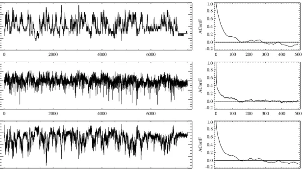
inFigure4 show diagnosticvariablesof the simulatedpointprocess, namely the number
of points and the log-posterior and log-prior densities. Though the autocorrelation is
reasonablylow, the mixingofthe algorithmmay be improved, for instance by simulated
tempering (Geyer and Thompson, 1995). The acceptance probabilities for the dierent
movetypes are listed inTable 2.
0
2000
4000
6000
5
10
15
20
25
Number of points
0
100
200
300
400
500
-0.2
0.0
0.2
0.4
0.6
0.8
1.0
ACorrF
0
2000
4000
6000
-4200
-4000
-3800
-3600
-3400
-3200
Log-posterior density
0
100
200
300
400
500
-0.2
0.0
0.2
0.4
0.6
0.8
1.0
ACorrF
0
2000
4000
6000
-120
-100
-80
-60
-40
Log-prior desity
0
100
200
300
400
500
-0.2
0.0
0.2
0.4
0.6
0.8
1.0
ACorrF
Subsample no.
Lag
Figure 4: Time seriesof summary statistics obtained by subsamplingevery 10th iteration of
the modied MCMC algorithm. Left: Simulatedvaluesof the number of points, log-posterior
and log-priordensities. Right: Empiricalauto-correlationfunctionsforthe timeseries.
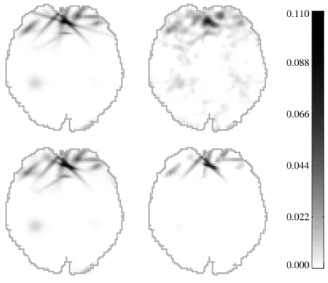
TheimagesinFigure5showtheposteriormeanactivationlevel,calculatedvoxel-wise
in the present model with uncorrelated noise and in a model with a separable
spatio-temporal correlation function to be described later. The area with high activation
in-tensity in the back of the brain corresponds wellwith the visual cortex, which is known
to process visual impressions. Displayed for comparison is also the non-parametric
es-timate with kernel-width 3 voxels (FWHM). The problemwith oversmoothing seems to
be present also in this example, though the true scene is not known for these data. On
the other hand, the posterior mean images possess some very eccentric regions, which
are most likely artifacts. The simplistic noise model is one likely reason for this. This
is both intuitively clear, since it is well known that the noise may be complex in fMRI
data, and can also be seen by comparing the improvement in the estimatein the model
Table 2: Acceptance probabilitiesforthe dierent move types inthe MCMCalgorithm. The
correlated noisemodelwillbedescribed inSection6.2.
Move type Acceptance (%) Acceptance (%)
Independent noise Correlated noise
Insert point 15.7 13.9 Deletepoint 15.6 14.1 Update position 10.6 11.5 Update height 40.8 45.2 Update area 30.6 34.3 Update angle 64.7 66.6 Update ratio 55.9 59.4
suggest that more elaboratednoise modelling is akey factor in addressing this, and will
discuss an extension to correlated noise in Section6.2. Another approach is to penalize
eccentric ellipsesmore in the prior distribution. This seems sensible, since relativelyfew
voxels are aected by a thin ellipse, and thus the likelihood function contains little
in-formation onthese. One problem,however, is the fact that the imaged slice is a section
through theconvolutedcorticalsurface. Eccentric ellipsesmaythusarise naturallywhen
a circular area on the cortical surface is transected orthogonally by the image-plane. A
natural,but alsomuch more ambitiousextension, is thusto extract the geometry of the
corticalsurface fromhigh-resolutionanatomical scans, and formulate the modeldirectly
on the two dimensional surface. Recent works along this line are Andrade et al. (2000)
and Kiebelet al. (2000).
A more fundamental dierence between the model-based and non-parametric
ap-proach, is the possibility of attaching estimates of uncertainty to the images. As an
example of this, displayed is also a conservative activation estimate, obtained by
sub-tractingtwo timesthe voxel-wise standard deviationfromthe meanimage. Thismay be
considered asa thresholded versionof the originalmean image,but wherethe threshold
isvoxel-dependent,toreect the voxel-wise uncertainty. This isonlyone possible way of
visualizingthe posteriorvarianceof activationpattern, and the exibilityof the MCMC
approach may of coursebeexploited ina range of other ways. One possibility isto
esti-mate summary characteristics of the activation pattern with associated standard errors,
whichmaybeused toquantify howwelldata supportspecic neuroscientic hypothesis.
6 Extensions
SofarwehaveestablishedabasicframeworkforanalyzingfMRIdatabyasimple
spatio-temporal model. However, both the noise and signal may possess more complex
struc-tures, which this model does not account for, necessitating several renements and
0.000
0.022
0.044
0.066
0.088
0.110
Figure5: Activation estimatesforthevisualstimulationdata. Top: Meanposterioractivation
inthestochasticgeometrymodelwithuncorrelatednoise(left)andthenon-parametricestimate
with kernel-width 3 voxels (right). Bottom: Mean posterior activation in the model with a
separablespatio-temporalcovariancefunctiondescribedinSection6.2(left),andaconservative
estimate in this model, obtained by subtracting twice the standard deviation from the mean
activation levelineach voxel(right).
6.1 Non-stationary responses
Wehaveassumedthatthetemporalpattern'isthesameforallvoxels,toobtainasimple
spatio-temporalmodel. It is well known, that this is only an approximation, and more
general approaches are studied for instance by Lange and Zeger (1997) and Genovese
(2000), who explicitly account for dierences in delay from one voxel to another. In
practice, the approximation will be relatively good for blocked paradigms, where the
stimulus is presented for longer periods of time, but problematic for so-called
event-related designs,where the presentation changesrapidly. A natural extensionto improve
this, istolinearly combinethe simpleresponsefunction with itsderivativeswith respect
todierentparameters(Fristonetal.,1998). Thesemay,inaTaylor-likefashion,account
for small voxel-visedierences inthe delay and dispersion.
Afundamentalquestion,whichismorechallengingtoaddress,iswhethertheresponse
the state-space model ' t = t + t ; t t 1 N(0; 2 ); t=1;2;:::;m; (14) where f t t 1
g are independent and
0
= 0. The mean
t
is the simple model (3)
which reects the overall temporal structure, but ' is allowed to deviate from this via
therandomwalkstructureofthenoiseterms
t
. Thevariance 2
governsthesmoothness
of the residual process '
t
t .
Bycombiningthiswiththespatialprior(2),wecanmakeinferenceon(X;') through
the joint posterior distribution P(X;'jY). For computational reasons we will in fact
consider the posterior of (X;';), where = f
i
;i 2 Vg are the random intercepts in
the model (4). This isgiven by
p(X;';jY)/P(YjX;';)P(X)P(')P();
wherethelikelihoodtermisobtainedbyconditioningonin(4). AMarkovchainwiththe
posterior as invariantdistribution may begenerated by a variable-at-a-time
Metropolis-Hastings algorithm, where iteratively one parameter is updated given the two others.
When updating X the proposals are as described earlier, though with the modication
that we replace A i (x) with A i (x)+ i and set 2
= 0 in the formulas in Section 4 to
condition on . A similar modication applies to the likelihood function in (5), when
calculating the acceptance ratio. When updating or ' we can simulate directly from
the conditional distributions,as it can easilybe veriedthat
i jY;X;'N 2 2 + 2 =ss ' ( ~ Y i A i (X)); 2 1 2 2 + 2 =ss ' ; (15) withall i
'sconditionallyindependent. Thesimulationof'maybecarriedoutrecursively
by simulating (' t j' t+1 ;:::' m
;X;;Y) for t = m;m 1;:::;1. These are all normal
distributions,and the momentsmay be calculated eÆciently with the Kalmansmoother
(West and Harrison, 1989).
We estimated the temporal response using the visual stimulation data of Section 2,
thoughpreprocessedinaslightlydierentway,asweremoved somelow-frequencytrends
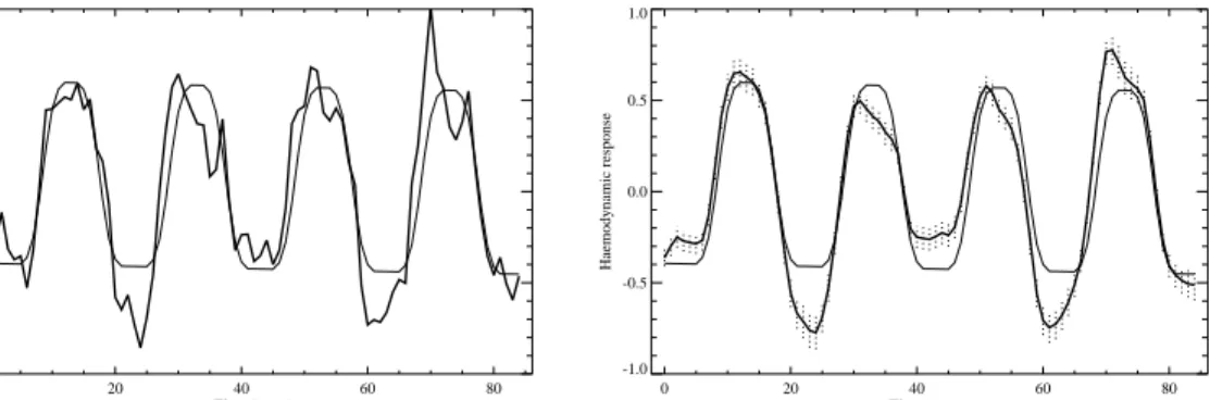
withlarge magnitudetostabilizethe algorithm. The plotsinFigure6illustrateasimple
least squares estimate and the posterior mean of ' . The simple estimate is obtained
by assuming that the spatial activation pattern isxed and given by the meanimage in
the top left panel in Figure 5. The posterior mean is based on75000 simulationsof the
Markov chain described above, where the update rules for the points are as in Section
5.2. Bothplots indicatethat the actualresponse may infactnot be described by axed
time-invariant model as the last peak is higher than the three rst, and the dip below
baselineis more prominentafter the rst and third cycle than afterthe second.
A consequence of modelling ' in this way, is that the stimulation function is only
partlyincludedinthemodel. ThoughitmayseemineÆcienttoignorearelevantcovariate
like this, in some experiments the actual stimulation is not directly controllable by the
0
20
40
60
80
Time (scans)
-1.0
-0.5
0.0
0.5
1.0
Haemodynamic response
0
20
40
60
80
Time (scans)
-1.0
-0.5
0.0
0.5
1.0
Haemodynamic response
Figure 6: Left: Least squares estimate of the haemodynamic response, assuming a known
spatialactivationpatterngiven bythetopleft panelinFigure5. Right: MonteCarlo estimate
of the posterior mean of the haemodynamic response function based on 7500 subsamples of
75000 iterations of the MCMC algorithm (see text.) Overlaid are pointwise 95%-credibility
regions based on the posterior variance. The initial stationary model (3) is overlaid as a thin
lineinbothplots.
timepoint. Furthermorewiththis formulation,wemaydetectsubtleactivationpatterns,
which depends on the paradigm inmore complex ways. An example of the latter is the
XORsignal of Lange et al. (1999).
Asafurtherextensionacollectionofdierentresponsefunctionscouldbemodelledby
a multidimensionalstate space modelfor'. Byassigningdierentfunctions todierent
groups of centres, one may account for regionaldierences in the response. At least for
moderate dimensions of 'the recursive simulation routinewould still be very eÆcient.
6.2 Correlated noise
As discussed earlier the initial model with uncorrelated noise is too simple in practice.
The noise sourcesin fMRI data are both of physiological and physical origin. The pixel
values are constructed by inverse Fourier transforms of measurements of currents in a
coil overa short time period. Hence there is no physical separation of the pixels, which
could justify independence. The temporal correlation arises from physiological sources,
but alsointrinsicallyin the MR scanner.
The main problemwith modelling a general covariance function is the fact that the
likelihoodfunction must beeasilycalculated, in order thatthe MCMC algorithmis
rea-sonablyfast. Atractablestartingpointistoassumeaseparablecovariancefunction. We
havepreviouslystudiedthe empiricalcorrelation ofthe visualstimulationdata (Hartvig,
1999),and found evidencethat the temporalcovariancevariedslightly withspatial
loca-tion, but that a separable modelwas a reasonable approximation tothe true covariance
function. Letting " = f"
it
;i 2 V;t = 1;:::;mg be the noise terms in (4) regarded as a
jVjm matrix, we willthus consider the model
"N (0; 2
wheredenotes the Kroneckerproduct andwhere and are the spatialandtemporal
correlation matricesof dimension jVjjVj and mm, respectively.
LetLandM denotethe lower-triangularCholeskysquare rootsof and . Consider
the data Y as a jVjm matrix and let Y Æ = Y(M 1 ) 0 , and ' Æ = M 1 '. Then the
conditional likelihoodfunction,where we condition on,is given by
p(Yjx;';)=(2 2 ) mjVj 2 jMj jVj jLj m exp ( 1 2 2 m X t=1 kL 1 (Y Æ ?t ~ Y Æ ' Æ t )k 2 ) exp 1 2 2 =ss Æ ' kL 1 ( ~ Y Æ A )k 2 ; (16) where ~ Y Æ i = m X t=1 Y Æ it ' Æ t =ss Æ ' and ss Æ ' = m X t=1 ' Æ t 2
are dened equivalently to (6), and Y Æ ?t = fY Æ it g i2V
. Notice that equations of the form
v = L 1
w may be solved easily, due to the lower-triangularity of L. Suppose good
estimates are available for and , such that the uncertainty of these can be ignored.
By simplyinserting the expression above in the Metropolis-Hastingratio insteadof (5),
the MCMC algorithmwill converge to the posterior distribution in the correlated noise
model.
The problemis thus reduced to obtainingestimates of and , orrather the
corre-spondingCholesky decompositionsof these. Duetothe largenumberofvoxels, itis
gen-erallyveryhardtodecompose,whichprecludetheuseofGaussianmodelsparametrized
intermsofelementsofthecovariancematrix(Cressie,1991). Asapragmaticalternative,
inHartvig(1999)weproposedastationarymovingaverage-typemodel,parametrized
di-rectly by L. For a given ordering of the voxel indices (corresponding to the ordering of
the elements of the matrix ), we let L
ij = l i j , where l k = 0 unless k 2 D and D is a
set of neighbours in the positive direction. We chose the lexicographic ordering of voxel
indices, and though the covariance function will to some extend depend on this choice,
the computationaladvantagesofparametrizingthemodel interms ofLareconsiderable:
By construction, the covariance function will always be positive denite, which
simpli-es parameter estimation, and both the covariance and inverse covariancematrices may
easilybecalculated, despite the large dimensionality.
We tted a stationary model with six parameters to the spatial covariance and an
AR(1)-modeltothe temporalcovariancefunction. Usingthe visualstimulationdata, we
performed 75000 iterations of the MCMC algorithm as described in Section 5.2. The
mean posterior activation image is displayed in Figure 5, and as discussed earlier, it is
slightly improved compared to the originalestimate.
6.3 Negative haemodynamic responses
We have restricted the activation level a
k
that an area is more active during the \rest"-condition than the stimulation condition,
or it may be attributed to special haemodynamic eects. In order to extend the model
to account for this, the activation may be represented as A +
A , where A +
and A
are positive surfaces describing positive and negative activationrespectively. For
identi-ability reasons we have to incorporate an interaction term in the prior that separates
the two surfaces; if not, overlapping positiveand negativesites willbehighlycorrelated,
and the interpretationof the activation surface becomes very diÆcult.
We propose simplyto use an interaction prior, which makes the two surfaces
condi-tionallyindependentgiven thedata. Forthe independent noisemodel, theprior isof the
form p(X + ;X )/f(X + )f(X )exp ( X i2V A i (X + )A i (X ));
wheref()isthedensityin(2)andwhereX +
andX aretwopointprocessesdetermining
the positive and negative surfaces respectively. When > 0, the last term penalizes
conguration where A i (X + ) and A i
(X ) are both large for some i 2 V. Let 1 = 2 =ss ' + 2 , the variance of ~ Y i
, then it is easy to see that X +
and X are independent
given the data Y. Hence we can make inference about X +
and X in their respective
marginaldistributions, and afterwards combine estimates using the independence of the
two point processes. Clearly other types of interactions may be considered, but the
present is appealing because of the advantages of marginalizing the inference, namely a
reduction of the dimensionality of the point processes and improved properties of the
simulation algorithm.
6.4 Interaction between centres
In Bayesian object recognition it is well known, that unless an interaction term is
in-cludedinthe prior, the estimatemay tendtocontain clustersof almostidentical objects
(Baddeley and van Lieshout, 1993). An extension of the prior in this respect may have
the followingform
p(x)/ n Y k=1 ( k ) Y k<j (x k ;x j ) n Y k=1 (p(a k )p(d k )p(r k )); x2;
where is an interaction function, which prevents centres from clustering. It is natural
to consider a function with a hard-core property, which prohibits pairs of centres with
distances close to zero. This is achieved with the modelof Ogataand Tanemura (1984)
where (x k ;x j ) = 1 expf (Æ(x k ;x j )=) p
g; p 2; with respect to a distance Æ(;)
on X. Here > 0 is an interaction radius. A hard-core Strauss model is obtained
by setting p = 1, while nite values of p yield an interaction function which increases
continuously from 0 to 1 with the distance between two points. A natural denition of
the distance Æ is to let two centres be close, if they are close in space and have similar
size and shape. One way of assessing this is by the J-divergence (Kullback,1959) of the
correspondingGaussianfunctions. Thisdoesnotsatisfythe triangleequality,andisthus
6.5 Generalization to three dimensions
The spatial model can straightforwardly be generalized to a three dimensional setting
where S R 3
. In this case a centre is given by x = (;a;d;r
1 ;r 2 ; 1 ; 2 ); and the
contributionto the activation volume is
h(i;x)=aexp log2 4 3d 2=3 j 2 1 (r 2 1 =r 2 r 3 ) 2=3 + j 2 2 (r 2 2 =r 1 r 3 ) 2=3 + j 2 3 (r 2 3 =r 1 r 2 ) 2=3 : Here r 3 =1 r 1 r 2 , r k >0for k =1;2;3and (j 1 ;j 2 ;j 3 )= 0 @ cos 1 cos 2 sin 1 cos 1 sin 2 sin 1 cos 2 cos 1 sin 1 sin 2 sin 2 0 cos 2 1 A (i ):
Withthis parametrizationdisthevolumeofthecontourellipsoidatheighta=2,and r
k is
theratioofthe kthmainaxisandthesumofthe threeaxes. Theangles
1 and
2
are the
rotations in the xy-plane and xz-plane respectively, which are restricted to the interval
[ =4;=4]. The natural extension of the priors is to assume that (r
1 ;r 2 ) D 2 ( r ; r ) where D 2
is the twodimensional Dirichlet distribution.
7 Discussion
We have proposed a spatio-temporalmodel for fMRI data which explicitly accounts for
thefactthatsignalchangesarelocallycoherentinbothspaceandtime. Thisassumption
isoftenimplicitlyincludedintheanalysis,whenspatialandtemporallteringareapplied,
but rarely formulated explicitly ina model. The relation(5) shows that in the simplest
setting we are eectively tting Gaussian functions of dierent sizes and orientations
to a regression image, and assessing the signicance of these. The random eld theory
has counterparts to this, namely the search for local maxima in both scale and space
(Siegmund andWorsley, 1995),andinthe spaceof ellipseswithdierentorientationand
shape (Shae et al., 1998). The method is, however, fundamentally dierent from the
random eld approach. The latter providesa framework for signal detection, by testing
multiple null hypotheses with correction for the large number of tests performed. As
was pointed out by Keith Worsley in the discussion to Lange and Zeger (1997), what is
reallyanestimation problemis thusanswered by hypothesis testing,with corresponding
conceptual and mathematicalproblems. With the proposed method the focus is shifted
towards estimationof the activation pattern by standard Bayesian methods.
Since the amountof data in fMRIexperiments maybeenormous, there is a
compro-mise between model complexity and the computational burden of the analysis. In an
attempt to formulate a relatively simple model, we have made specic assumptions on
the spatial pattern, and clearly these may not be fully satised by the true activation.
Though the random intercept surface willaccount forminor deviations fromthe point
As mentioned earlier, Kiebel et al. (2000) and Andrade et al. (2000) have recently
studied global models, where the geometry of the cortical surface is used to model the
haemodynamiceects. Thesewerenotformulatedinaparametricframework,and
assess-ingthe uncertainty of estimated activation patterns were not considered. The geometry
of the cortical surface is a very relevant covariate to be included in our setup also, for
instance by formulating the model on the two dimensional surface. A major challenge
with this extension, however, is the increased computationalburden, whichis alreadyat
the limitof what is acceptable forpractical purposes.
Alternatively local spatial models have been proposed by Descombes et al. (1998),
Salli et al. (2001) and Hartvig and Jensen (2000). These are Markov random eld-type
models, whereMAPestimates are obtained iterativelyorinclosedform,whence MCMC
isnotrequired. The computationalburden isthusmuchreduced, butsoisthe inferential
scope, since only a point estimate is obtained. In the present setup, the signicance of
hypothesesofinterestwithinsinglesubjectsmaybequantied,orestimatesandstandard
errors ofrelevantfeatures ofthe activationindierentexperimentsmay beobtained, for
comparing dierent groups of subjects.
Modelling the temporal response in a non-parametric setting with few assumptions
seemsrelevant,giventhe uncertainty aboutthe haemodynamiceects indierent
stimu-lationtypes. Alsothefactthatthemodelledresponsedependsonlypartlyonthespecied
paradigmis anadvantage when analyzingdata wherethe actualparadigmis diÆcultto
determine. Theapproachhassomesimilaritywithnon-parametricmultivariatemethods,
suchasprincipalcomponentanalysis (PCA),where arepresentativetime courseand the
correspondingspatialpatternisestimateddirectlyfromthedata. Inoursetup, the
time-course is also estimated from the data, but unlike in PCA, the assumptions of spatial
smoothnessand coherency is simultaneously taken intoaccount.
Withnoticeableexceptions (Genovese, 2000;Franketal.,1998), Bayesian analysesof
fMRI data are rare. We are of the opinion that a Bayesian approach to this data makes
sense for several reasons. Firstly there is substantialprior informationon the activation
pattern, which should of course be used in the analysis. This may either be general
knowledgeof thefunctionalorganizationof thebrain, orresults fromearlierexperiments
on the same subject. The ease by which data can be acquired even allows us to design
experiments according to this, by performing pilot studies to generate detailed prior
information before the actual experiment. Secondly often large inter- and intra-subject
variation is observed, which makes it more natural to consider the activation pattern
as a realization of stochastic variable than as a xed unknown parameter. A similar
interpretation is made in the currently applied random eect analyses of Holmes and
Friston (1998).
Acknowledgements
This work was supported by MaPhySto, Centre for Mathematical Physics and
Waagepetersen. Thanks to Hans Stdkilde-Jrgensen from the MR-ResearchCentre at
Skejby Sygehus for kindly providingthe data, and toan anonymous referee for valuable
suggestions for improving the paper.
References
Andrade, A.,Kherif, F., Mangin, J.F.,Worsley,K.J., Simon, O., Dehaene, S., LeBihan,
D.andPoline,J.B.(2000)DetectionoffMRIactivationusingcorticalsurfacemapping.
Research report, Service HospitalierFrederic Joliot, CEA, Orsay. Submitted.
Baddeley,A.J.andvanLieshout,M.N.M.(1993)Stochasticgeometrymodelsinhigh-level
vision.In K.V. Mardia and G.K. Kanji (eds.), Statistics and Images, vol. 1, chap. 11,
pp. 231{256,Appl. Statist.
Boynton,G.M.,Engel,S.A.,Glover,G.H.andHeeger,D.J.(1996)Linearsystemsanalysis
of functionalmagnetic resonance imagingin human V1. J. Neurosci., 16, 4207{4221.
Bullmore, E., Brammer, M., Williams, S.C., Rabe-Hesketh, S., Janot, N., David, A.,
Mellers, J., Howard, R. and Sham, P. (1996) Statistical methods of estimation and
inferencefor functional MRimage analysis. Magn. Reson. Med., 35, 261{277.
Buxton, R.B., Wong, E.C. and Frank, L.R. (1998) Dynamics of blood ow and
oxy-genationchangesduringbrain activation: Theballoonmodel. Magn.Reson.Med., 39,
855{864.
Cressie,N.A.C. (1991)Statistics for spatial data.Wiley SeriesinProbabilityand
Mathe-maticalStatistics: Applied Probabilityand Statistics. New York: John Wiley& Sons,
Inc.
Descombes, X.,Kruggel,F.andvonCramon,D.Y.(1998)fMRIsignalrestorationusinga
spatio-temporalMarkov randomeld preserving transitions. NeuroImage, 8,340{349.
Frank, L.R., Buxton, R.B. and Wong, E.C. (1998) Probabilistic analysis of functional
magnetic resonance imagingdata. Magn. Reson. Med., 39, 132{148.
Friston, K.J., Jezzard, P. and Turner, R. (1994) The analysis of functional MRI
time-series.Human Brain Mapping,1, 153{171.
Friston, K.J., Holmes, A.P., Poline, J.B., Grasby, P.J., Williams, S.C.R., Frackowiak,
R.S.J. and Turner, R. (1995) Analysis of fMRI time-series revisited. NeuroImage, 2,
45{53.
Gaschler-Markefski,B.,Baumgart,F.,Tempelmann,C.,Schindler,F.,Stiller,D.,Heinze,
H.J.andScheich,H.(1997)Statisticalmethodsinfunctionalmagneticresonance
imag-ing with respect to nonstationary time-series auditory cortex activity. Magn. Reson.
Med., 38,811{820.
Genovese, C.R. (2000) A Bayesian time-course model for functionalmagnetic resonance
imaging data. J. Amer. Statist. Assoc., 95, 691{719. With discussion and a reply by
the author.
Geyer, C.J. and Mller, J. (1994) Simulation procedures and likelihood inference for
spatialpoint processes. Scand. J. Stat., 21, 359{373.
Geyer, C.J. and Thompson, E.A. (1995) Annealing Markov chain Monte Carlo with
applicationsto ancestral inference.J. Amer. Statist. Assoc., 90,909{920.
Green,P.J.(1995)ReversiblejumpMarkovchainMonteCarlocomputationandBayesian
modeldetermination.Biometrika,82, 711{732.
Hartvig, N.V. (1999) A stochastic geometry model for fMRI data. Research report 410,
Departmentof Theoretical Statistics, University of Aarhus.
Hartvig, N.V. (2000) Parametric Modelling of Functional Magnetic Resonance Imaging
Data.Ph.D. thesis, Department of TheoreticalStatistics, University of Aarhus.
Hartvig, N.V. and Jensen, J.L. (2000) Spatial mixture modelling of fMRI data. Human
Brain Mapping, 11,233{248.
Holmes, A.P. and Friston, K.J. (1998) Generalisability, random eects and population
inference.NeuroImage, 7, S754.
Holmes, A.P., Josephs, O., Buchel, C. and Friston, K.J. (1997) Statisticalmodelling of
low-frequency confounds in fMRI.NeuroImage, 5, S480.
Kiebel,S.J., Goebel,R. and Friston,K.J. (2000) Anatomicallyinformedbasis functions.
NeuroImage,11, 656{667.
Kullback, S. (1959)Information Theory and Statistics. John Wiley & Sons, Inc.
Kwong, K.K.,Belliveau,J.W., Chesler,D.A., Goldberg,I.E. et al.(1992)Dynamic
mag-netic resonance imaging of human brain activity during primary sensory stimulation.
Proc. Natl. Acad. Sci. USA,89, 5675{5679.
Lange,N.(1996)Tutorialinbiostatistics.Statisticalapproachestohumanbrainmapping
by functionalmagnetic resonance imaging.Statistics in Medicine,15, 389{428.
Lange,N. andZeger, S.L.(1997) Non-linearFouriertimeseries analysisforhumanbrain
Lange, N., Strother, S.C., Anderson, J.R., Nielsen, F.A., Holmes, A.P., Kolenda, T.,
Savoy, R. and Hansen, L.K. (1999) Plurality and resemblance in fMRI data analysis.
NeuroImage,10, 282{303.
Ogata, Y. and Tanemura, M. (1984) Likelihoodanalysis of spatial point patterns. J. R.
Statist. Soc. B, 46, 496{518.
Press, W.H., Teukolsky, S.A., Vetterling, W.T. and Flannery, B.P. (1992) Numerical
Recipes in C. Cambridge University Press, second edn.
Salli,E.,Korvenoja, A., Visa, A.,Katila, T. and Aronen, H.J. (2001)Reproducibility of
fMRI:Eect of the use of contextual information.NeuroImage, 13, 459{471.
Shae,K., Worsley,K.J.,Wolforth,M.andEvans,A.C.(1998)Rotationspace: Detecting
functionalactivationbysearchingoverrotatedand scaledlters.NeuroImage, 7,S755.
Siegmund,D.O.andWorsley,K.J.(1995)Testingforasignalwithunknown locationand
scale ina stationaryGaussian randomeld. Ann. Stat.,23, 608{639.
West, M. and Harrison, J. (1989) Bayesian Forecasting and Dynamic Models.
Springer-Verlag, New York.
Worsley,K.J.(1995)EstimatingthenumberofpeaksinarandomeldusingtheHadwiger
characteristic of excursion sets, with applications to medical images. The Annals of
Statistics, 23, 640{669.
Worsley, K.J. and Friston, K.J. (1995) Analysis of fMRI time-series revisited | again.