Wright State University
Wright State University
CORE Scholar
CORE Scholar
Browse all Theses and Dissertations
Theses and Dissertations
2017
OCLEP+: One-Class Intrusion Detection Using Length of Patterns
OCLEP+: One-Class Intrusion Detection Using Length of Patterns
Sai Kiran Pentukar
Wright State University
Follow this and additional works at: https://corescholar.libraries.wright.edu/etd_all
Part of the Computer Engineering Commons, and the Computer Sciences Commons
Repository Citation
Repository Citation
Pentukar, Sai Kiran, "OCLEP+: One-Class Intrusion Detection Using Length of Patterns" (2017). Browse all Theses and Dissertations. 1758.
https://corescholar.libraries.wright.edu/etd_all/1758
This Thesis is brought to you for free and open access by the Theses and Dissertations at CORE Scholar. It has been accepted for inclusion in Browse all Theses and Dissertations by an authorized administrator of CORE
OCLEP+: ONE-CLASS
INTRUSION DETECTION
USING LENGTH OF PATTERNS
A thesis submitted in partial fulfilment of the requirements for the degree of
Master of Science
By
SAI KIRAN PENTUKAR
B.Tech., Jawaharlal Nehru Technological University, 2012
2017
WRIGHT STATE UNIVERSITY GRADUATE SCHOOL
May 18, 2017 I HEREBY RECOMMEND THAT THE THESIS PREPARED UNDER MY SUPERVISION BY
Sai Kiran PentukarENTITLEDOCLEP+: One-Class Intrusion Detection Using Length of Patterns BE ACCEPTED IN PARTIAL FULFILLMENT OF THE REQUIREMENTS FOR THE DEGREE OFMaster of Science.
Guozhu Dong, Ph.D. Thesis Director
Mateen Rizki, Ph.D.
Chair, Department of Computer Science & Engineering Committee on Final Examination Guozhu Dong, Ph.D. Junjie Zhang, Ph.D. Bin Wang, Ph.D.
Robert E.W. Fyffe, Ph.D.
ABSTRACT
Pentukar, Sai Kiran. M.S., Department of Computer Science and Engineering, Wright State Uni-versity, 2017. OCLEP+: One-Class Intrusion Detection Using Length of Patterns.
In an earlier paper, a method calledOne-class Classification using Length statistics of (jumping) Emerging Patterns (OCLEP)was introduced for masquerader detection.
Jumping emerging patterns (JEPs) for a test instance are minimal patterns that match the test instance but they do not match any normal instances.
OCLEP was based on the observation that one needs long JEPs to differentiate an instance of one class from instances of the same class, but needs short JEPs to differentiate an instance of one class from instances of a different class.
In this thesis, we presentOCLEP+, One-class Classification using Length statistics of Emerging Patterns Plusby adding several new ideas to OCELP. OCLEP+ retains the one-class training feature of OCELP, hence it only requires the normal class data for training. Moreover, OCELP+ has the advantage of being not model or signature based, making it hard to evade. OCLEP+ uses only length statistics of JEPs, making it a robust method. Experiments show that OCELP+ is more accurate than OCLEP and one-class SVM, on the NSL-KDD datasets.
Contents
1 Introduction 1
2 Preliminaries 3
2.1 Discretization . . . 3
2.2 Emerging Patterns . . . 3
2.3 Border Differential Algorithm . . . 4
3 Concepts of OCLEP+ 5 3.1 Why length of EPs is more important for ID . . . 5
3.2 Define Length Statistics (LS) . . . 6
3.3 Framework of OCLEP+ . . . 6
3.4 How OCLEP+ builds classifiers using the LS features . . . 7
3.5 Illustration of OCLEP+ . . . 8
4 Experiment Evaluation 11 4.1 Datasets used in the experiment . . . 11
4.2 Data used in experiments and for training . . . 11
4.3 Competing algorithms used . . . 12
4.4 Accuracy of algorithm . . . 12
4.4.1 Experiment A. . . 14
4.4.2 Experiment B. . . 15
4.5 Cutoff and selected parameter values . . . 16
4.6 Impact of parameters. . . 17
4.6.1 Choosingk . . . 17
4.6.3 Choosingl . . . 19
5 Related Works 21 5.1 One Class SVM. . . 21
5.2 OCLEP . . . 21
5.3 Difference between OCLEP and OCLEP+ . . . 22
5.4 OCLEP+ vs Other multi class training classifiers . . . 22
5.5 Other Works . . . 23
6 Discussion and Future Works 24
Appendices 25
Bibliography 27
List of Figures
4.1 OCLEP+: ROC curve for experiment A . . . 15
4.2 OCLEP+: ROC curve for experiment B . . . 16
4.3 Experiment results of the algorithm for different values ofk . . . 18
4.4 Experiment results of the algorithm for different values ofr . . . 19
4.5 Experiment results of the algorithm for different values ofl . . . 20
List of Tables
3.1 Sample dataset of normal instances. . . 8
3.2 Mapping table for example dataset . . . 9
3.3 Discretized sample dataset of normal instances . . . 10
4.1 Description of datasets for training and testing . . . 12
4.2 Experiment A: TP, FP, TN and FN comparison. . . 14
4.3 Experiment A: Comparison of OCLEP+ . . . 14
4.4 Experiment B: TP, FP, TN and FN comparison. . . 15
4.5 Experiment B: Comparison of OCLEP+ . . . 16
4.6 Choosingk: Evaluation results . . . 17
4.7 Choosingr: Evaluation results . . . 18
4.8 Choosingl: Evaluation results . . . 20
1 Symbols table . . . 26
1
Introduction
In a world where the usage of the Internet has become an integral part of many organizations’ operations, effective intrusion detection systems (IDS) are becoming increasingly important, for protecting these organizations from the ever growing risk of cyber threats.
Current IDS have major weaknesses, because they are mostly signature based or model based, or they require both the normal and intruder data to train their IDS classifier.
In this thesis we present a robust and effective method, namely OCLEP+, One-class Classification using Length statistics of Emerging Patterns Plus, that overcomes the above weaknesses. At a high level, OCLEP+ uses length statistics of jumping emerging patterns (JEPs) to detect anomalies, and importantly, by One-class we mean that OCLEP+ uses only normal data to train its detection engine.
Given a test instance x, JEPs are minimal patterns (given as conditions on attributes) that match xbut they do not match any of the normal data instances [2][4][5]. We note that JEPs are not frequent patterns, as they only match one instance. OCLEP+ is based on the observation that one often needs long JEPs to differentiate an instance s of a class from set of N instances of the same class, but often needs very short JEPs to differentiate an instancexof one class from a set of
N instances of other class.
OCLEP+ uses minimal length statistics of the lengths of JEPs concerning a test instance. Cutoff on these statistics is obtained using the normal data instances in the training process.
OCLEP+ has several advantages over other approaches: it has better accuracy compared to One-Class SVM; it is easy to train as it requires only the normal class data for training; it is hard to evade by the intruders as it is not model or signature based approach. Being able to train
2 with only normal class data is significant for building an IDS engine because it is hard to collect anomaly class data, especially when an organization is in the initial stages of incorporating IDS in its infrastructure. These features imply that OCLEP+ is an excellent choice to consider for a robust intrusion detection system.
While OCLEP+ started from OCLEP [2], it contains several new features which make it more accurate and robust. These will be detailed later.
In the rest of this thesis, chapter2 presents all required preliminaries. In chapter3, the Length Statistics are defined and the OCLEP+ algorithm is discussed. It also presents an illustration of the OCLEP+ algorithm. Chapter 4 discusses the dataset used for evaluation and presents evaluation results comparing OCLEP+ against One Class SVM and OCLEP. Chapter5 discusses about One Class SVM, OCLEP and also about other works related to one class classification methodology. Finally, in Chapter6 we discuss the summary of the thesis and also possible future works.
2
Preliminaries
2.1
Discretization
Discretization is the process of transforming quantitative data into qualitative data [7]. It can also be defined as the process of transforming numerical attributes into a small number of intervals. Even though quantitative data can be used for learning classifiers, qualitative data is needed for pattern mining and it can also add value when building classifiers [14].
Discretization can be achieved by many to one mapping of the quantitative data to a qualitative value. An example is to discretize values for age into categories such as 20-39, 40-59, and 60-79. Let’s consider the following records for age attribute: 10, 20, 24, 25, 32, 35, 36, 40. Then our discretization categories could be (-Inf 10], (10 20], (20 30], (30 40], (40 Inf). Then the discretized mapping for 10 would be A, 20 would be B, 24 → C, 25 → C, 32 → D, 35 → D, 36 → D, 40 → D.
Commonly used discretization methods include equi-width, equi-depth, and entropy based meth-ods. In this algorithm we are using equi-width discretization method.
2.2
Emerging Patterns
We use the concept of emerging patterns (EPs) [4] [6] in OCLEP+. EPs are patterns whose support in one class is very high compared to the support in the other class. Growth rate of emerging patterns [2] is defined as the ratio of its support in one class over the support in another. Given two datasets D1 andD2, for each pattern X we define suppd1(X) as the support of X in D1 and
similarlysuppd2(X) as the support of X in D2. Then the growth rate (GR) of patternX [5] from
2.3. BORDER DIFFERENTIAL ALGORITHM 4 GR(X) =
0 ifsuppd1(X) = 0 andsuppd2(X) = 0
∞ ifsuppd1(X) = 0 andsuppd2(X)6= 0 suppd2(X)
suppd1(X) otherwise.
The emerging patterns with growth rate of∞are called as Jumping Emerging Patterns [4]. In this thesis, for jumping emerging pattern mining, we have D1 = {s} consisting of just one
data instance andD2is a set of normal class instances.
2.3
Border Differential Algorithm
In this thesis, we use a simplified version of border differential algorithm [4]. Border differential algorithm accepts a discretized instance t and a set of normal discretized instancesT. Below, we view each discretized instance as a set of items.
The following is our simplified version of border differential algorithm, BorderDiff(t,T):
1. Compute the differences: Assume that T ={t1, t2, t3, t4, ..., tn}.
For eachi, letdi=t−ti
2. Eliminate non minimal sets in{d1, ..., dn}: A non minimal set is a set in {d1, ..., dn} that is a
super set of other sets in{d1, ..., dn}. It can be proven that non minimal sets lead to increased
computation time but they do not have any impact on the results of this algorithm.
3. Compute cross product and minimization iteratively: Let cp1 ={{x1, x2} |x1 ∈d1, x2 ∈d2}.
Then fori= 2, ..., n,
Compute“crossproduct”(cpi) ={X∪ {xi} |X ∈cpi−1and xi∈di}
and remove all non minimal sets fromcpi.
e.g.M in({1,123,15,14,234,45,235,5}) ={1,234,5}
3
Concepts of OCLEP+
We now introduce our OCLEP+ method for intrusion detection. In a nutshell, OCLEP+ uses one class training data, i.e. a set of normal instances to train the classifier and build some EP length statistics, and then makes classification decision based on the length statistics obtained for the test instances.
3.1
Why length of EPs is more important for ID
To answer this question, letD1andD2 be two different classes of data in a dataset. Let us pick an
instancet1fromD1and pick a subsetT1ofD1− {t1}and computeBorderDif f(t1, T1). Let us also
pick another instancet11 fromD2and pick a subsetT11fromD1and computeBorderDif f t11, T11
. Under the assumption that data of a particular class are similar to each other,BorderDif f(t1, T1)
yields longer patterns and BorderDif f t1 1, T11
yields short patterns. The reason behind is that sincet1 and T1 belong to the same class, it needs long patterns to differentiate them and since t11
andT1
1 are from different classes, they require very short patterns to differentiate.
This leads to the conclusion that instances from same class yields long patterns and instances from different classes yields short patterns1. This is helpful for intrusion detection because, as we
are training our classifier with the normal data instances and any other instance from the normal class yields long patterns and an instance from the anomaly class yields short patterns. Thus using the length statistics of the patterns obtained, we can successfully classify if an instance is normal or anomaly class data.
3.2. DEFINE LENGTH STATISTICS (LS) 6
3.2
Define Length Statistics (LS)
In this thesis, we use the following length statistics to differentiate a normal and an anomaly class data.
The minimum length for an instances is defined as the length of the pattern, which is shortest of all the patterns generated by the border differential algorithm for s. According to the concept of emerging patterns, data from the same class have long minimal length and data from different classes have short minimal length. As we are training our classifier with normal data, any other instance from normal class yield patterns of longer length and instance from the anomaly class yield shorter patterns.
Given each instance s, an integerr >0, and a setTi of instances of the normal class, we define
M inLen(s) =M in({|p| |p∈
r
[
i=1
BorderDif f(s, Ti)})
We note that we run theBorderDif f() algorithmrnumber of times which will be discussed in section3.3, hence the r in the above formula. To calculate the minimal length of all the patterns, we collect the patterns generated at each round and choose the pattern with shortest length of all the patterns.
3.3
Framework of OCLEP+
The following is the algorithm to train the OCLEP+ classifier.
Algorithm 1OCLEP+ Training
pick a random setS ofkinstances from N foreachsin S do
foreachiin {1...r} do
pick a random subsetTi ofl instances from N− {s}
compute BorderDiff(s, Ti) end
ComputeM inLen(s) =M in({|p| |p∈S7
i=1BorderDif f(s, Ti)}) end
3.4. HOW OCLEP+ BUILDS CLASSIFIERS USING THE LS FEATURES 7 Remark 1: k is the number of random instances we choose to train our algorithm. OCLEP+ is such that it doesn’t require to compute the length statistics for all the instances of normal class. You get the same classification parameters even if you perform the training for all instances of normal class training-data or calculate for a decent number of instances. In our experiments,kis chosen to be 800 based on our experimental results in section4.6.1.
Remark 2: ris the number of timesBorderDif f() is computed for the same instance. For every round of BorderDif f(), we collect the emerging patterns obtained and choose the pattern with minimal length of all the rounds ofBorderDif f() to compute the minimal length, length statistics as described in section 3.2. r is required to eliminate the probability of false length statistics obtained due to few records that are labeled as anomaly but similar to the normal class data. In our experiments based on the results in section 4.6.2we chooser= 7.
Remark 3: lis the size of random instances(T) set chosen fromN (set of normal data) for every instance which we want to classify. It’s chosen such that if the size ofN is small,lis|(N)−1|. But ifN is considerably large, then l can be any number like 300, 500 etc. For the NSL-KDD dataset we choosel to be 400 based on our experimental results described in section4.6.3.
The following is algorithm to use the OCLEP+ classifier on a test instance.
Algorithm 2OCLEP+ Testing For a testing instance,x
foreachiin {1...r} do
pick a random subsetTi ofl instances from N
compute BorderDiff(x,Ti) end
ComputeM inLen(x) =M in({|p| |p∈S7
i=1BorderDif f(x, Ti)}) if M inLen(x)≥cutof f obtainedintraining then
Classifyxas normal instance;
else
Classifyxas anomaly instance;
end
3.4
How OCLEP+ builds classifiers using the LS features
3.5. ILLUSTRATION OF OCLEP+ 8 value to differentiate a normal instance from an anomaly. The cutoff value for the minimum length statistics to determine if an instance is normal or anomaly class is chosen such that 5 percentile of the training length statistics are more than the cutoff value.
3.5
Illustration of OCLEP+
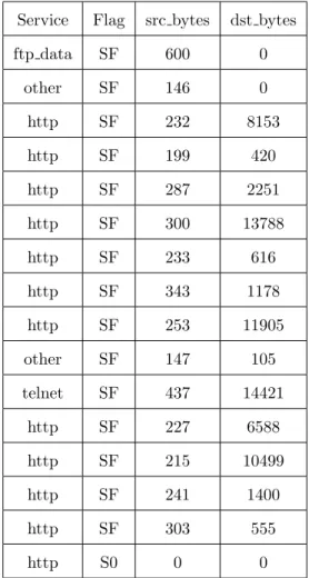
The following is an illustration of OCLEP+ algorithm. To explain the algorithm we chose 4 features from NSL-KDD dataset, which is the dataset we used for our experiment evaluation. The features we chose for this illustration are,service, flag, src bytes, dst bytes. The following Table3.1is a one class normal data with the 4 chosen features.
Service Flag src bytes dst bytes
ftp data SF 600 0 other SF 146 0 http SF 232 8153 http SF 199 420 http SF 287 2251 http SF 300 13788 http SF 233 616 http SF 343 1178 http SF 253 11905 other SF 147 105 telnet SF 437 14421 http SF 227 6588 http SF 215 10499 http SF 241 1400 http SF 303 555 http S0 0 0
Table 3.1: Sample dataset of normal instances
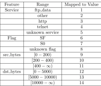
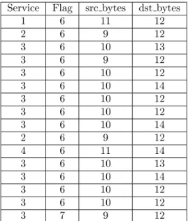
As described in section 2.1, the above table need to be discretized to efficiently perform the classification using OCLEP+. Table3.3is the discretized table of the above dataset which is derived
3.5. ILLUSTRATION OF OCLEP+ 9
Feature Range Mapped to Value
Service ftp data 1 other 2 http 3 telnet 4 unknown service 5 Flag SF 6 S0 7 unknown flag 8 src bytes [0−200) 9 [200−400) 10 [400− ∞) 11 dst bytes [0−5000) 12 [5000−10000) 13 [10000− ∞) 14
Table 3.2: Mapping table for example dataset
based on the mapping reference table3.2.
Let’s consider an instance which belongs to the same normal class and apply border differential algorithm on it.
http SF 255 861
The discretized form of the above example would be the following.
3 6 10 12
Application of border differential algorithm as described in section3.3yields us an emerging pattern of length 2 which is{10,12}.
Lets consider another transaction which belongs to the anomaly class and apply border differen-tial algorithm on it.
supdup S0 0 0
The discretized form of the above example would be the following.
5 7 9 12
Application of border differential algorithm yields us an emerging pattern of length 1 which is{5}. It can be observed that application of OCLEP+ algorithm on the normal instance with the normal class data gave us an emerging pattern of longer length, however attack instance with normal class data gave us an emerging pattern of shorter length. Based on this significant jumping emerging
3.5. ILLUSTRATION OF OCLEP+ 10
Service Flag src bytes dst bytes
1 6 11 12 2 6 9 12 3 6 10 13 3 6 9 12 3 6 10 12 3 6 10 14 3 6 10 12 3 6 10 12 3 6 10 14 2 6 9 12 4 6 11 14 3 6 10 13 3 6 10 14 3 6 10 12 3 6 10 12 3 7 9 12
4
Experiment Evaluation
4.1
Datasets used in the experiment
We use the NSL-KDD dataset1 to evaluate OCLEP+ classifier. NSL-KDD is an improved version of KDDCUP’99 dataset2. KDD-Cup is the data set used for The Third International Knowledge Discovery and Data Mining Tools Competition, which was held in conjunction with KDD-99 (The Fifth International Conference on Knowledge Discovery and Data Mining). The KDDCUP dataset includes a wide variety of intrusions that are simulated in a military network environment. This dataset was widely used in evaluating many intrusion detection algorithms but it suffers from many disadvantages such as having many redundant records because of which the results were more biased towards the algorithms that are based on frequency of records. NSL-KDD addressed the disadvan-tages of KDDCUP by removing all the duplicate records [12]. Moreover, the records were selected such that the percentage of records is inversely proportional to the difficulty level thus promoting more accurate evaluation of different learning techniques [12].
4.2
Data used in experiments and for training
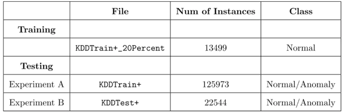
One of the main features of OCLEP+ is that it requires only one class, i.e normal class instances, to train the classifier. NSL-KDD dataset provides aKDDTrain+_20Percent file that contains both anomaly as well as normal instances with 41 features to train the Intrusion Detection classifiers. To train our classifiers, we separated the normal instances from the file and trained our classifiers with
1NSL-KDD: http://www.unb.ca/cic/research/datasets/nsl.html
4.3. COMPETING ALGORITHMS USED 12 the 13499 normal instances thus obtained.
We use two different datasets to evaluate the classifier trained from the set of 13499 normal instances as described above. In Experiment A, all the 125973 instances of the KDDTrain+ file which includes both the normal and also the anomaly instances are tested with our classifiers. In Experiment B, we use theKDDTest+file which contains 22544 instances to evaluate our classifier.
File Num of Instances Class
Training
KDDTrain+_20Percent 13499 Normal
Testing
Experiment A KDDTrain+ 125973 Normal/Anomaly
Experiment B KDDTest+ 22544 Normal/Anomaly
Table 4.1: Description of datasets for training and testing
4.3
Competing algorithms used
In this section, OCLEP+ is compared against One Class SVM with linear, polynomial, and RBF kernels, and also OCLEP. The reason to choose the above three versions of SVM for evaluation is that they are very popular and also use only one class normal data to train the classifier; we do not consider many other classifiers and techniques since they use multi-class data, which is both the normal as well as anomaly data, to train their classifier.
4.4
Accuracy of algorithm
Precision, recall, F-score and Accuracy are the metrics we use to compare the prediction performance of the algorithms. For any classification algorithm, there can be a possibility of four classification cases and these help to understand the difference between various metrics that we use.
1. True Positives (TP): The number of positive instances predicted as positives. 2. False Positives (FP): The number of negative instances predicted as positives. 3. True Negatives (TN): The number of negative instances predicted as negatives.
4.4. ACCURACY OF ALGORITHM 13 4. False Negatives (FN): The number of positive instances predicted as negatives.
Accuracy can be defined as the proportion of the correct results that are achieved by the classifier.
Accuracy= (T P+T N)/(T P +T N+F P +F N)
Though accuracy is a good metric to determine the prediction performance of a classifier, it alone cannot be used to determine the prediction performance because it suffers from accuracy paradox and as it does not consider the false positives and false negatives of a classifier, it can be tricked to produce better accuracy result despite producing a poor prediction performance. This is especially true when the two classes are not balanced.
Precision helps to determine the number of actual positive data accurately predicted out of all the data predicted as positive by the classifier. It can be defined as,
P recision=T P/(T P +F P)
A high precision of a classifier means that it is really good at not classifying the normal data as positive (anomaly). A less precision mean that there are lot of normal data that are falsely predicted as positive.
Recall helps to determine the number of actual positive data accurately predicted out of all the positive data. It can be defined as,
Recall=T P/(T P+F N)
A high recall rate means that all the positive data are accurately predicted as positive. A less recall rate mean that there are more positive data that are determined as normal data by the classifier.
F-score is the harmonic mean of both recall and precision and it helps to give a better indication of the prediction performance of a classifier. It can be defined as,
4.4. ACCURACY OF ALGORITHM 14
4.4.1
Experiment A
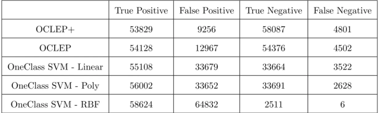
Table4.3 is the comparison of above discussed metrics for OCLEP+ against One Class SVM with linear, polynomial, RBF kernels, and also OCLEP. As it can be observed, the F-score of OCLEP+ is 2% above that of OCLEP. It can also be observed that One class SVM often gives more recall rate compared to OCLEP and also OCLEP+ but it fails to give good precision accuracy. Figure4.1
presents the ROC curve of OCLEP+ classifier for experiment A.
True Positive False Positive True Negative False Negative
OCLEP+ 53829 9256 58087 4801
OCLEP 54128 12967 54376 4502
OneClass SVM - Linear 55108 33679 33664 3522
OneClass SVM - Poly 56002 33652 33691 2628
OneClass SVM - RBF 58624 64832 2511 6
Table 4.2: Experiment A: TP, FP, TN and FN comparison
Precision Recall F-score Accuracy
OCLEP+ 85.33 91.81 88.45 88.84
OCLEP 80.67 92.32 86.11 86.13
OneClass SVM - Linear 62.07 93.99 74.76 70.47
OneClass SVM - Poly 62.46 95.52 75.53 71.20
OneClass SVM - RBF 47.49 99.99 64.39 48.53
4.4. ACCURACY OF ALGORITHM 15
Figure 4.1: OCLEP+: ROC curve for experiment A
4.4.2
Experiment B
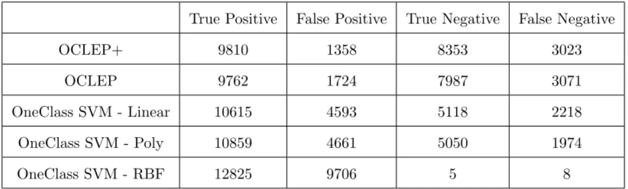
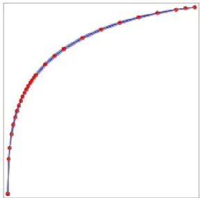
Table4.5summarizes the experimental results for OCLEP+, OCLEP, One Class SVM with linear, polynomial, and RBF kernels. It can be observed that OCLEP+ stands out with the best results compared to other algorithms. Figure4.2 presents the ROC curve for experiment B.
True Positive False Positive True Negative False Negative
OCLEP+ 9810 1358 8353 3023
OCLEP 9762 1724 7987 3071
OneClass SVM - Linear 10615 4593 5118 2218
OneClass SVM - Poly 10859 4661 5050 1974
4.5. CUTOFF AND SELECTED PARAMETER VALUES 16
Precision Recall F-score Accuracy
OCLEP+ 87.84 76.44 81.75 80.57
OCLEP 84.99 76.07 80.28 78.73
OneClass SVM - Linear 69.80 82.72 75.71 69.79
OneClass SVM - Poly 69.97 84.62 76.60 70.57
OneClass SVM - RBF 56.92 99.94 72.53 56.91
Table 4.5: Experiment B: Comparison of OCLEP+
Figure 4.2: OCLEP+: ROC curve for experiment B
Based on the above two experimental evaluation results, it can be concluded that OCLEP+ stands out as an algorithm with good recall rate and also an acceptable precision which makes it more robust algorithm compared to One Class SVM.
4.5
Cutoff and selected parameter values
In section3.3, we introduced 3 parametersk,r, andlthat we use in our algorithm. In the following section, we will discuss the chosen values for the parameters and also the cutoff value obtained in our experiment to make classification decision.
Based on the results obtained in section 4.6, and many more experiments with various combi-nation of parameter values, it was observed that optimal results are obtained whenk= 800,r= 7
4.6. IMPACT OF PARAMETERS 17 and l = 400. The cutoff value of minimal length statistics obtained by OCLEP+ algorithm with those parameters in place is 3. Any instance which on application of OCLEP+ testing algorithm generating a pattern with minimal length of 3 or more is classified as normal or anomaly otherwise.
4.6
Impact of parameters
In this section, we discuss how the different parameters of the algorithm; k, r and l which are discussed in section3.3 are chosen. Our experiments show that the evaluation results are optimum whenk= 800,r= 7 andl = 400. We ran a series of experiments to choose the right values which is discussed below.
4.6.1
Choosing
k
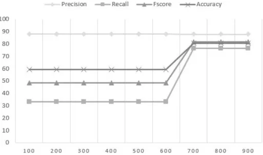
We ran the experiment with different values ofk by choosingl= 400 andr= 7 as constants. The results of experiment are shown in table4.6. It can be observed from the experimental results that we got optimum result for k ≥ 700. So we chose k to be 800. The reason is, as we are training with fewer instances, the cutoff value is not accurate and it would be less than or equal to 2, which means all instances generating an emerging pattern with length 2 are also falsely identified as normal instances.
k TP FP TN FN FPR TPR Precision Recall F-score Accuracy
100 4301 565 9146 8532 0.06 0.34 88.39 33.52 48.60 59.65 200 4301 565 9146 8532 0.06 0.34 88.39 33.52 48.60 59.65 300 4301 565 9146 8532 0.06 0.34 88.39 33.52 48.60 59.65 400 4301 565 9146 8532 0.06 0.34 88.39 33.52 48.60 59.65 500 4301 565 9146 8532 0.06 0.34 88.39 33.52 48.60 59.65 600 4301 565 9146 8532 0.06 0.34 88.39 33.52 48.60 59.65 700 9822 1360 8351 3011 0.14 0.77 87.84 76.54 81.80 80.61 800 9822 1360 8351 3011 0.14 0.77 87.84 76.54 81.80 80.61 900 9822 1360 8351 3011 0.14 0.77 87.84 76.54 81.80 80.61 1000 9822 1360 8351 3011 0.14 0.77 87.84 76.54 81.80 80.61
4.6. IMPACT OF PARAMETERS 18
Figure 4.3: Experiment results of the algorithm for different values ofk
4.6.2
Choosing
r
We ran the experiment withr ranging from 1 to 10 withk = 800 and l = 400 as constants. The results of experiment are shown in table 4.7. It can be observed based on the figure 4.4 that the result curve is almost flat fromr= 5. So we chooser= 7 to make sure we get optimum results.
r TP FP TN FN FPR TPR Precision Recall F-score Accuracy
1 9127 976 8735 3706 0.10 0.71 90.34 71.12 79.59 79.23 2 9515 1136 8575 3318 0.12 0.74 89.33 74.14 81.03 80.24 3 9656 1231 8480 3177 0.13 0.75 88.69 75.24 81.42 80.45 4 9727 1279 8432 3106 0.13 0.76 88.38 75.80 81.61 80.55 5 9766 1312 8399 3067 0.14 0.76 88.16 76.10 81.69 80.58 6 9787 1348 8363 3046 0.14 0.76 87.89 76.26 81.67 80.51 7 9807 1358 8353 3026 0.14 0.76 87.84 76.42 81.73 80.55 8 9814 1374 8337 3019 0.14 0.76 87.72 76.47 81.71 80.51 9 9838 1384 8327 2995 0.14 0.77 87.67 76.66 81.80 80.58 10 9831 1408 8303 3002 0.14 0.77 87.47 76.61 81.68 80.44
4.6. IMPACT OF PARAMETERS 19
Figure 4.4: Experiment results of the algorithm for different values ofr
4.6.3
Choosing
l
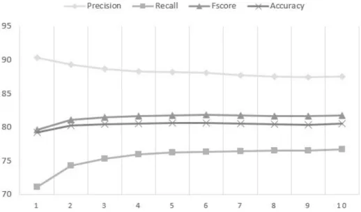
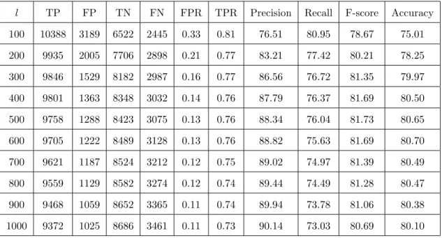
We ran the experiment withl ranging from 100 to 1000. The results of the experiment are shown in table 4.8. It can be observed that increasing l results in poor recall rate but improvement in precision. It can also be observed that the F-score is maximum atl = 400. So we chose l = 400 for this experiment. The reason for F-score to again decline after l = 500 is that, larger T from
4.6. IMPACT OF PARAMETERS 20
l TP FP TN FN FPR TPR Precision Recall F-score Accuracy
100 10388 3189 6522 2445 0.33 0.81 76.51 80.95 78.67 75.01 200 9935 2005 7706 2898 0.21 0.77 83.21 77.42 80.21 78.25 300 9846 1529 8182 2987 0.16 0.77 86.56 76.72 81.35 79.97 400 9801 1363 8348 3032 0.14 0.76 87.79 76.37 81.69 80.50 500 9758 1288 8423 3075 0.13 0.76 88.34 76.04 81.73 80.65 600 9705 1222 8489 3128 0.13 0.76 88.82 75.63 81.69 80.70 700 9621 1187 8524 3212 0.12 0.75 89.02 74.97 81.39 80.49 800 9559 1129 8582 3274 0.12 0.74 89.44 74.49 81.28 80.47 900 9468 1059 8652 3365 0.11 0.74 89.94 73.78 81.06 80.38 1000 9372 1025 8686 3461 0.11 0.73 90.14 73.03 80.69 80.10
Table 4.8: Choosingl: Evaluation results
5
Related Works
Throughout our experiment evaluation phase we compared our algorithm against One Class SVM and also OCLEP. So in this section we discuss about one class SVM, OCLEP and also all other related work done on NSL-KDD data using one class classifiers.
5.1
One Class SVM
Support Vector Machines aremaximal margin classifiers. In the training phase, the One Class SVM algorithm maps input data, which is of single (one) class, into a high dimensional feature space via a kernel function and iteratively identifies the hyperplane that separates training data from origin with a maximum margin[8]. Now the one class problem is transformed into a two class problem, where all the training data lies in one class and the origin is the second class.
We evaluated One Class SVM using LIBSVM 3.22 [1] software with Linear, Polynomial and RBF kernels (with default settings). For intrusion detection problem on NSL-KDD dataset and using all the 41 features of dataset, it can be observed in table 4.3 and 4.5 that OCLEP+ and OCLEP outperformed One Class SVM.
5.2
OCLEP
OCLEP was first introduced in [2]. It was originally evaluated for the masquerader detection prob-lem but it was unable to outperform One Class SVM for that probprob-lem. However because it is configuration free and requires little tuning when compared to One Class SVM, it has been widely recognized. In this thesis, the same algorithm was used for the evaluation of intrusion detection
5.3. DIFFERENCE BETWEEN OCLEP AND OCLEP+ 22 problem and it was able to outperform One Class SVM. The reason is, one of the main features of NSL-KDD dataset is that it doesn’t include redundant records and it has been noted in [2] that OCLEP performs better than one class SVM when there are more unique instances and in-case there are more redundant instances, then one class SVM performs better. As NSL-KDD dataset which was used for evaluation doesn’t have redundant records, OCLEP was able to outperform one class SVM.
5.3
Difference between OCLEP and OCLEP+
Both OCLEP and OCLEP+ are based on length statistics of emerging patterns. However, several improvements on OCLEP are presented in this thesis which resulted in better performance for the intrusion detection problem. The following are major differences between OCLEP and OCLEP+. (1) OCLEP+ classifier uses the minimal length feature of the emerging patterns while average length was used in OCLEP. (2) OCLEP+ algorithm computes BorderDiff() for every instance multiple times (4.6.2) to improve the robustness of classifier. (3) OCLEP failed to provide a definitive way to choose the cutoff to classify an instance. In fact it was stated that any numbercsatisfyinga≤c≤bwhere
aandb are the minimum and maximum of the average lengths of the emerging patters obtained by Borderdiff() algorithm, can be used as a cut-off threshold. In contrast, OCLEP+ chooses its cut-off by choosing a number that satisfies 5 percentile Length Statistics of the training data (4.5).
5.4
OCLEP+ vs Other multi class training classifiers
[12] compared the accuracy of other famous algorithms like J48, Naive Bayes, NB Tree, Random Forest, Multi-layer Perceptron and SVM on the KDDTest+ dataset which we used for our Ex-periment B. It can be noted in figure 5.1 that the accuracy of most of the classifiers are close to OCLEP+, which has an accuracy of 80.57%.
Even though J48, NB Tree, Random Forest and Random tree produce slightly better accuracy compared to OCLEP+ classifier, OCLEP+ is more practical to implement as it needs only one class data to train the classifier.
5.5. OTHER WORKS 23
Figure 5.1: Accuracy of other multi class classifiers
5.5
Other Works
There are several other algorithms that achieved better accuracy compared to OCLEP+ on NSL-KDD dataset, but those algorithms used two class data for training.
[9] was able to achieve 81.2% of accuracy for the classification problem, but they trained their classifier with two class data, i.e both anomaly, normal. Their other evaluation metrics are; Recall: 69.35; Precision: 96.59; F-score: 80.74. OCLEP+ was able to outperform their algorithm both in recall rate and also F-score.
[10] mentioned that they were able to achieve 92.16% of recall rate which is pretty impressive but it leaves behind many discrepancies. The author mentioned they were testing against 23238 instances but NSL-KDD test dataset which is KDDTest+ has only 22544 records. Moreover they proposed a one class classifier and also evaluated against One Class SVM, but they mentioned that they are using both normal, anomaly class data to train their classifier (”In this paper we have proposed a One-class small hypersphere support vector machine classifier (OCSHSVM) algorithm, which builds a learning classifier model via both normal and abnormal network traffic.”), which effectively mean they are using two class data to train their classifier and also all the anomaly and normal instances they included in training the One Class SVM classifier are considered belonging to the same class
6
Discussion and Future Works
In this thesis we introduced a new improved classification algorithm, OCLEP+ and applied our classifier to the Intrusion Detection problem. OCLEP+ is a one class classifier that requires only one class data for its training. It generates EPs based on only normal class data and calculates classification cutoff for the minimal length statistics. It has been demonstrated that OCLEP+ can achieve very good detection rate compared to the previous algorithm, OCLEP, One Class SVM and also other algorithms that used two class data for its training. OCLEP+ doesn’t need anomaly class data for its training and also as it is also not a model based approach, it is hard to evade by the intruders. All the above results and features imply that OCLEP+ is more robust and effective intrusion detection system.
Intrusion detection is a hard problem. Everyday many new attacks can happen and the attacks may involve the use of new features. Being able to train the classifier with one class data is very important because of the diversified nature of these attacks. We might never have enough data to train our classifier if we rely on anomaly class data for training.
We used all the 41 features of the NSL-KDD dataset to evaluate the performance of our algorithm. Possible future work could be to test the performance of the classifier using few selected features of the dataset. And OCLEP+ can be tested for other data mining problems like document classification [11], web page classification [13], image retrieval [3], fall detection [15] and check performance of the classifier.
26 Table 1: Symbols table
Symbol Meaning Symbol Meaning
OCLEP+ One Class Classification using OCLEP One Class Classification using
Length statistics of Emerging Length Statistics of Emerging
Patterns Plus Patterns
IDS Intrusion Detection System JEP Jumping Emerging Pattern
x Instance of anomaly class data s Instance of normal class data
EP Emerging Pattern GR Growth Rate
N Normal dataset T Subset ofN
k Number of random instances to get the r Number of timesBorderDif f() length statistics for training the classifier computer for same instance
l Size of T SVM Support Vector Machine
RBF Radial Basis Function TP True Positive
FP False Positive TN True Negative
FN False Negative FPR False Positive Rate
References
Chih-Chung Chang and Chih-Jen Lin. LIBSVM: A library for support vector machines. ACM Transactions on Intelligent Systems and Technology, 2:27:1–27:27, 2011. Software available at http://www.csie.ntu.edu.tw/~cjlin/libsvm.
Lijun Chen and Guozhu Dong. Masquerader detection using OCLEP: One class classification using length statistics of emerging patterns. In Int’l Workshop on Information Processing over Evolving Networks (WINPEN), 2006.
Yunqiang Chen, Xiang Sean Zhou, and T. S. Huang. One-class svm for learning in image re-trieval. InProceedings 2001 International Conference on Image Processing (Cat. No.01CH37205), volume 1, pages 34–37 vol.1, 2001.
Guozhu Dong and Jinyan Li. Efficient mining of emerging patterns: Discovering trends and differences. In Proceedings of the Fifth ACM SIGKDD International Conference on Knowledge Discovery and Data Mining, KDD ’99, pages 43–52, New York, NY, USA, 1999. ACM.
Guozhu Dong and Jinyan Li. Mining border descriptions of emerging patterns from dataset pairs.
Knowl. Inf. Syst., 8(2):178–202, 2005.
Guozhu Dong, Jinyan Li, L. Wong, and Limsoon Wong. The use of emerging patterns in the analysis of gene expression profiles for the diagnosis and understanding of diseases, 2003. S. Garca, J. Luengo, J. A. Sez, V. Lpez, and F. Herrera. A survey of discretization techniques: Taxonomy and empirical analysis in supervised learning. IEEE Transactions on Knowledge and Data Engineering, 25(4):734–750, April 2013.
Katherine A. Heller, Krysta M. Svore, Angelos D. Keromytis, and Salvatore J. Stolfo. One class support vector machines for detecting anomalous windows registry accesses. In Proc. of the workshop on Data Mining for Computer Security, 2003.
28 B. Ingre and A. Yadav. Performance analysis of nsl-kdd dataset using ann. In2015 International Conference on Signal Processing and Communication Engineering Systems, pages 92–96, Jan 2015.
S. Kumar, S. Nandi, and S. Biswas. Research and application of one-class small hypersphere support vector machine for network anomaly detection. In 2011 Third International Conference on Communication Systems and Networks (COMSNETS 2011), pages 1–4, Jan 2011.
Larry M. Manevitz and Malik Yousef. One-class svms for document classification. J. Mach. Learn. Res., 2:139–154, March 2002.
M. Tavallaee, E. Bagheri, W. Lu, and A. A. Ghorbani. A detailed analysis of the kdd cup 99 data set. In 2009 IEEE Symposium on Computational Intelligence for Security and Defense Applications, pages 1–6, July 2009.
Hwanjo Yu, Jiawei Han, and Kevin Chen-Chuan Chang. Pebl: Positive example based learning for web page classification using svm. InProceedings of the Eighth ACM SIGKDD International Conference on Knowledge Discovery and Data Mining, KDD ’02, pages 239–248, New York, NY, USA, 2002. ACM.
Nayyar A. Zaidi, Yang Du, and Geoffrey I. Webb. On the effectiveness of discretizing quantitative attributes in linear classifiers. CoRR, abs/1701.07114, 2017.
Tong Zhang, Jue Wang, Liang Xu, and Ping Liu. Fall Detection by Wearable Sensor and One-Class SVM Algorithm, pages 858–863. Springer Berlin Heidelberg, Berlin, Heidelberg, 2006.