Serial dependence in timing perception
Warrick Roseboom
Sackler Centre for Consciousness Science, Department of Informatics, University of Sussex, UK. [email protected]
Abstract
Recent sensory history affects subsequent experience. Behavioural results have demonstrated this effect in two forms: repeated exposure to the same sensory input produces negative after-effects wherein sensory stimuli like that previously experienced are judged as less like the exposed stimulation, while singular exposures can produce positive after-effects wherein judgements are more like previously experienced stimulation. For timing perception, there is controversy regarding the influence of recent exposure - both singular and repeated exposure produce apparently negative after-effects - often referred to as temporal recalibration and rapid temporal recalibration, respectively. While negative after-effects have been found following repeated exposure for all timing tasks, following a single exposure, they have only been demonstrated using synchrony judgements (SJ). Here, we examine the influence of a single presentation – serial dependence for timing – for standard timing tasks: SJ, temporal order judgements (TOJ), and magnitude estimation judgements (MJ). We found that serial dependence produced apparently negative after-effects in SJ, but positive after-effects in TOJ and MJ. We propose that these findings, and those following repeated exposure, can be reconciled within a framework wherein negative after-effects occur at sensory layers, consistent with classical depictions of sensory adaptation, and Bayesian-like positive after-effects operating across different, higher, decision levels. These findings are consistent with the after-effects known from other perceptual dimensions and provide a general framework for interpreting positive (serial dependence) and negative (sensory adaptation) after-effects across different tasks.
Significance statement
Perception of synchrony between audio and visual sensory inputs is critical to behaviour. It allows us to accurately perceive speech and determine causality. Previous work has shown that synchrony perception is affected by experience – having watched a movie wherein sound trailed vision, subsequent audio-visual experience is altered. Recently it was suggested that this change in experience occurs rapidly, following only brief exposure to out-of-sync audio-visual stimuli. Here we show that, while brief exposure changes synchrony perception, this change is not that same as that following prolonged exposure. To reconcile these results, we set out a hierarchy of perceptual processing: longer exposure changes basic sensory properties to improve perceptual precision; brief exposure affects higher-level decision processes to increase perceptual stability. These results are consistent with those in other sensory domains, such as visual orientation, suggesting that the brain uses similar processing strategies for audio-visual synchrony perception as in other cases.
Keywords: relative timing perception, serial dependence, rapid recalibration, temporal recalibration, sensory adaptation, audiovisual, multisensory
Perception of multisensory relative timing depends on the recent history of sensory exposure (see Linares et al., 2016 for review). Particularly for audiovisual relative timing, a large literature exists demonstrating that repeated exposure (up to several minutes of repeats) to a specific multisensory temporal relationship (e.g. audio-leads-vision by 200 ms) will produce changes in relative timing reports at least partially consistent with classic negative after-effects known in other sensory domains, such as the tilt or motion after-effects (Fujisaki et al., 2004; Vroomen et al., 2004; Di Luca et al., 2009; Roach et al., 2011; Roseboom et al., 2015). These relative timing after-effects, sometimes referred to as temporal recalibration, have been demonstrated regardless of the type of relative timing task used to examine them, including the most common relative timing tasks: synchrony judgments (SJ; Fujisaki et al., 2004; Vroomen et al., 2004), temporal order judgements (TOJ; Vroomen et al., 2004), and magnitude estimation judgements (MJ; Roach et al., 2011). Beyond single-interval appearance judgements, exposure-induced changes in the precision of audiovisual relative timing judgements, consistent with changes in appearance, have been reported in a three-interval oddity task (Roseboom et al., 2015).
More recently, several studies have reported that, at least for audiovisual relative timing, apparently negative after-effects can be found following only a single exposure – a so called rapid temporal recalibration (Van der Burg et al., 2013; 2015). This effect is revealed under a simple serial dependence approach, wherein, rather than having any explicit exposure period before participants produce responses, the response on a given trial is analysed depending on the stimulus value presented on the previous trial. Most surprisingly, the magnitude of this rapid negative after-effect is similar to that found following repeated exposure (see Figure 2B in Fujisaki et al., 2004 and Figure 1C in Van der Burg et al., 2013), suggesting that in the many previously reported studies, repeated exposure period was adding little to nothing to the magnitude of after-effect. This finding is unexpected for at least two reasons: First, among the putative mechanisms suggested to underlie the negative after-effect in audiovisual relative timing is adaptation of neural channels that selectively respond to the exposed stimulus (Roach et al., 2011). That a single exposure would produce the same amount of change in
neural response as repeated exposure seems a strange proposition. Moreover, it has been shown that the effect of repeated exposure gradually decreases given counter evidence (Machulla et al., 2012; Alais, Ho et al., 2017) rather than being immediately lost. If the same process underlies both effects, why an effect based on prolonged exposure would show a gradual decrease in effect size over time, but the same magnitude serial dependence could repeatedly appear instantly is a difficult issue to resolve.
The second reason that a rapid negative after-effect is unexpected is that serial dependence of reports typically produce the opposite kind of after-effect - a positive after-effect (Corbett et al., 2011; Liberman et al., 2014; Fischer & Whitney, 2014; Alais et al., 2015; Martin et al., 2015; Taubert et al., 2016a; Taubert et al., 2016b; Fritsche et al., 2017; Kiyonaga et al., 2017; Bliss et al., 2017; Suárez-Pinilla et al., 2018). These kinds of positive after-effects can be well accounted for by simple iterative Bayesian decision models that describe how previous experiences or reports can affect subsequent reports, and work across a wide range of sensory dimensions (Cicchini et al., 2014; Petzschner et al., 2015). It is unclear why serial dependence for audiovisual relative timing would be different from cases in all other sensory dimensions.
One potential point of interest is that, to our knowledge, the many studies showing a negative serial dependence in relative timing have used just one type of relative timing judgement – the SJ. As mentioned above, for audiovisual relative timing, repeated exposure modifies reports in all commonly used appearance tasks, and a measure of relative timing precision. These results are consistent with the prolonged exposure having produced adaptation of the sensory coding for relative timing (Roach et al., 2011; Roseboom et al., 2015). If the effect of a single exposure is the same as that for repeated exposure in relative timing, that is sensory adaptation, we should find a similar serial dependence in all tasks, not just the SJ. In this study, we examine serial dependence for the three common relative timing tasks – SJ, TOJ and MJ - using audiovisual stimuli.
Methods
Participants
Twenty participants (including WR) completed each experiment. The same 20 participants completed the simultaneity and temporal order judgement experiments, while only five participants completed all three experiments (Supplementary Material contains the raw data sorted by participant). Participant number is shared across data set so that if the participant number appears in multiple datasets, it refers to the same participant; 35 participants in total, 21 female, mean age 22.17, standard deviation 4.73). Written informed consent was acquired from all participants prior to the experiments, which were approved by the University of Sussex ethics committee. Participants volunteered their time, received £5 per hour, or course credit as compensation for their time.
Apparatus and materials
Participants sat in a quiet, bright room. Visual stimuli were displayed on an Iiyama Vision Master Pro 203 or LaCie Electron 22 Blue II monitor, with a resolution of 1024 x 768 pixels and refresh rate of 100 Hz. The monitor was positioned at a viewing distance of approximately 57 cm. Audio signals were presented binaurally through Sennheiser HDA 280 PRO headphones. Stimulus generation and presentation was controlled through Psychtoolbox 3 (Brainard, 1977; Pelli, 1997; Kleiner et al, 2007) run in MatLab (Mathworks, USA) on a desktop PC. Participants responded using the keyboard or mouse.
Visual events were luminance modulated Gaussian blobs (standard deviation 1.5 degrees of visual angle (dva)). Peak luminance difference from background was Michelson contrast 1 (Michelson, 1927); displayed against a grey (approx. 38 cd /m2) background. A fixation square (white approx. 76 cd /m2, subtending 0.25 dva) was presented centrally. The Gaussian blob was centred 3 dva above fixation. The visual stimulus was presented for one frame, approximating 10 ms in duration. Auditory signals
were a 10 ms amplitude pulse (square-wave, without ramping) of 1500 Hz sine-wave carrier at approximately 55 db SPL (measured monaurally inside headphone ear cup).
Design and procedures
As reports were unspeeded, different participants took more or less time to complete a given experimental session. All experimental sessions were constrained to a maximum of 1 hour of total participation. In the magnitude judgment experiment, all participants completed at least 5 sessions, though some completed six with each experimental session taking approximately seven minutes to complete. Simultaneity and temporal order judgement experiments consisted of 10 sessions, with each experimental session taking approximately five minutes to complete. In each session, participants were presented with a sequence of 90 audiovisual presentations. Each presentation consisted of visual and auditory events presented offset by one of nine pseudo-randomly selected stimulus-onset-asynchronies (SOAs)(±400, ±200, ±100, ± 50 and 0 ms; negative values indicate the auditory event appeared first), with each SOA presented 10 times, interspersed according to the method of constant stimuli. Each audiovisual presentation was preceded by a pseudo-random period of 500-1500 ms.
In the magnitude judgment experiment, following stimulus presentation a visual analogue scale appeared on the screen (e.g. Figure 1). Participants used the computer mouse to indicate the apparent temporal distance (in ms) between the auditory and visual stimuli. Prior to experimental sessions, participants completing the magnitude judgement experiment completed a practice session. Practice session details were similar to the experimental session except that the range of SOAs was different (±800, ±600, ±500, ±400, ±300, ±200, ±100, ± 50 and 0 ms) with each SOA presented only 5 times (85 trials in total). During practice sessions, following each trial, participants were shown text on the screen indicating the physical SOA of the previous trial, and their report in ms, with their report
following the text “Your response: …” and the physical SOA shown below following “Actual value: …”.
successive sessions of practice until the Pearson’s R of their reports relative to the physical SOA was
greater than 0.85 or until they had completed three sessions.
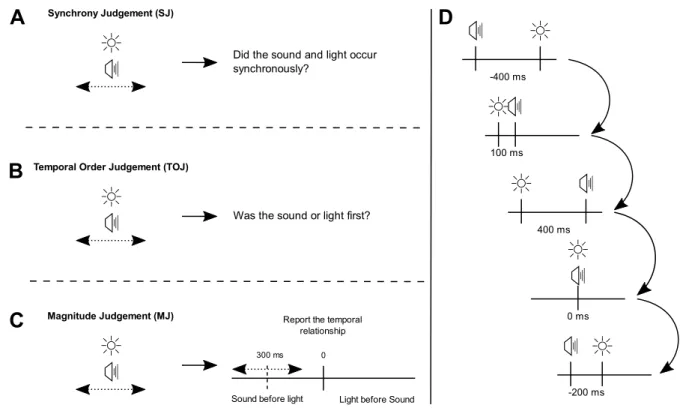
Figure 1. Schematics of the three relative timing tasks used and a trial sequence. A-C show the different questions that were asked of participants in each separate experimental session (SJ, TOJ, or MJ). D shows a sequence of audio visual relative timing trials. A response was required on every trial. Serial dependence is the influence of one trial on the next (arrows). We determined serial dependence in each task by splitting participant responses by the previous trial relative timing (e.g. audio-leads-vision by 400 ms, in the first depicted trial) and estimating the point of subjective synchrony for the subset of trials that immediately followed that value (e.g. vision-leads-audio by 100 ms in this case).
In the synchrony judgement experiment, participants provided an unspeeded response as to whether the auditory and visual events had occurred at the same time (synchronously; up cursor key) or not (asynchronously; down cursor key). In the temporal order judgement experiment, participants provided an unspeeded response as to whether the auditory or visual event had come first, audio (left
cursor key) or visual (right cursor key). No prior practice was given for synchrony or temporal order judgment experiments. When multiple experiments were completed by the same participants, for example the synchrony and temporal order judgment experiments, they completed each during separate experimental sessions on different days. The order of completion, synchrony or temporal order judgement experiment first, was counterbalanced across participants.
Hypothesis testing
Bayesian analyses were used to assess the relative evidence for (H1) or against (null; H0) the relevant hypotheses. We did not conduct any power analysis. Bayes factors evaluate the sensitivity of the obtained data to differentiate between the alternative (H1) and null (H0) hypotheses. Power relates to the application of a decision rule in the long run and so has no relevance to how sensitive the data are that have actually been collected (Dienes, 2014). Bayes factors can appropriately differentiate the sensitivity of the evidence to distinguish between hypotheses regardless of the applied stopping rule (Rouder, 2014; Schoenbrodt, et al., 2015).
Serial dependence across tasks
To investigate serial dependence for different relative timing judgements, for each judgement type
we split participants’ responses depending on the previously presented SOA (n-1 trial). This was done
in two ways: we split the data by whether the n-1 trial SOA had been negative (audio leads vision) or positive (vision leads audio), pooling across the different SOAs in those ranges. Each set of data for these two conditions was then fit with an appropriate model for estimating the point of subjective synchrony (PSS): a difference of cumulative Gaussians model for SJs (see Yarrow et al., 2011); and a cumulative Gaussian for TOJs (see Vroomen & Keetels, 2010) and MJs (Roach et al., 2011). These analyses were conducted in order to directly assess whether our results replicated those previously reported by Van der Burg and colleagues (2013) using SJs as this was the first method reported in that paper (page 14634, second paragraph of Results and Figure 1, Van der Burg et al., 2013). We further
analysed the data by splitting by each judgement type, participant, and n-1 trial SOA, again (as above) fitting the data with the appropriate model to estimate PSS. Statistical tests were carried out using
JASP (Version 0.8.3.1; JASP Team, 2018). Readers may disagree with the analysis approach and selection of prior for Bayesian analyses reported below. If so, the trial-wise data, by participant and task, is included in the Supplementary Material so that any alternative/further desired analyses can be conducted.
Synchrony Judgements
Each participant’s data was fitted with a difference of cumulative Gaussians with the PSS estimated as
the average of the synchrony criteria for audio-leads and vision-leads SOA (as per Yarrow et al., 2011; 2013). To confirm that our data displayed the same serial effects (rapid recalibration) as originally reported by Van der Burg and colleagues (2013) we examined the difference in PSS between when the previous trial had been negative and when it had been positive. This is the main test of serial effects reported in that paper. We estimated the effect size reported in that publication based on the outcome of the conducted frequentist T-test (t(14) = 3.6, p = 0.003) to be Cohen’s d = 0.9295. The direction of the effect was such that the PSS when the n-1 SOA had been positive was larger (35 ms) than when the n-1 SOA had been negative (15 ms). Consequently, from Van der Burg and colleagues’
result we could obtain both a predicted direction (PSS n-1 negative SOA < PSS n-1 positive SOA) and magnitude of effect (Cohen’s d = 0.9295). Using this information, we conducted a Bayesian paired-samples T-test on our data, with a prior defined by a half-normal distribution with a mean of 0 and standard deviation in effect size of 0.9295. This test revealed moderate evidence (BF-0 = 3.785) for the alternative hypothesis that there was a difference in PSS when the n-1 SOA been negative (mean PSS negative n-1 = 28 ms) versus when it had been positive (mean PSS positive n-1 = 46 ms). These results confirm that our data broadly replicated a similar effect in both size and direction as that previously reported.
As in Van der Burg et al (2013), we also compared the PSS following each n-1 SOA versus the PSS when the n-1 SOA was 0 ms. Two participants’ data was excluded from this analysis because the standard deviation of the fitted cumulative Gaussian for at least one synchrony criterion for one level of n-1 SOA exceeded the range of presented SOA for the criterion (400 ms), suggesting that the participant could not discriminate synchrony from asynchrony in that case. Figure 2A shows the average PSS for the remaining 18 participants, for trials following each n-1 SOA.
Figure 2. Average point of subjective synchrony (PSS) for 18 participants, estimated from SJs (A), TOJs (B) and MJs (C), depending on n-1 trial audiovisual SOA. Error bars depict standard error of the mean.
Van der Burg and colleagues (2013) reported frequentist T-tests comparing the PSS for n-1 SOAs where audio-leads-vision versus the PSS when n-1 SOA was 0 ms. Only the audio-leads-vision by 64 ms SOA was reported as significantly shorter (t(14) = 2.3, p = 0.034). This test provides an estimated effect size
of Cohen’s d = 0.5938 and an expected direction of effect such that the PSS for audio-leads-vision n-1
SOAs should be shorter than for n-1 SOA of 0 ms. The first row of Table 1 shows the results of Bayesian paired-samples T-tests between the PSS for each negative n-1 SOA level and the PSS when n-1 SOA was 0 ms. The prior was a half-normal distribution with a mean of 0 and a standard deviation in effect size of 0.5938. For the n-1 SOA levels of audio-leads-vision by 200, 100, and 50 ms, there was moderate evidence against the hypothesis that the PSS should be smaller than when the n-1 SOA was 0 ms. For the n-1 SOA of audio-leads-vision by 400 ms the evidence was insensitive. These results strengthen
the findings of Van der Burg and colleagues (2013) in showing clearly that there is evidence against a difference between negative and 0 ms n-1 SOAs (rather than the findings they report that there is no evidence for a difference, as p > 0.05), though partially contradict the finding at n-1 audio-leads-vision by 64 ms.
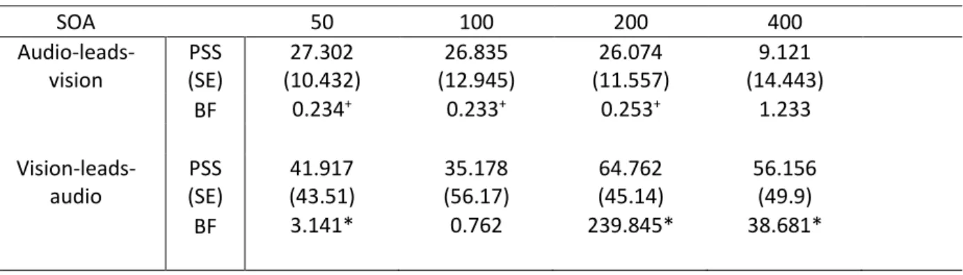
Table 1. PSS, standard error of the mean (SE), and Bayes Factor (BF) for Bayesian paired-samples T-tests comparing PSS when n-1 SOA was audio-leads-vision (first row) against PSS when n-1 SOA was 0 ms and the same for vision-leads-audio (second row). PSS when n-1 SOA was 0 ms was 20.859 (SE =
9.21). ‘+’ indicates evidence against the hypothesis that there was a directional difference between
conditions, while ‘*’ indicates evidence for this hypothesis.
SOA 50 100 200 400 Audio-leads-vision PSS (SE) 27.302 (10.432) 26.835 (12.945) 26.074 (11.557) 9.121 (14.443) BF 0.234+ 0.233+ 0.253+ 1.233 Vision-leads-audio PSS (SE) 41.917 (43.51) 35.178 (56.17) 64.762 (45.14) 56.156 (49.9) BF 3.141* 0.762 239.845* 38.681*
Taking the same approach for comparing PSSs where the n-1 SOA contained vision leading audio, Van der Burg and colleagues (2013) reported that all comparisons of these n-1 SOAs versus when n-1 SOA was 0 ms were significantly longer (ts(14) > 3.1, ps < 0.008). These results provide an estimated effect
size of Cohen’s d = 0.8 and an expected direction of effect such that PSS when n-1 SOA was
vision-leads-audio is larger than when n-1 SOA was 0 ms. The second row of Table 1 shows the results of Bayesian paired-samples T-tests between the PSS for each positive 1 SOA level and the PSS when n-1 SOA was 0 ms. The prior was a half-normal distribution with a mean of 0 and a standard deviation in effect size of 0.8. For the n-1 SOA levels of vision-leads-audio by 400, 200, and 50 ms, there was moderate evidence for the hypothesis that the PSS should be larger than when the n-1 SOA was 0 ms. For the n-1 SOA of vision-leads-audio by 100 ms the evidence was insensitive. Overall, these results are consistent with those reported by Van der Burg and colleagues (2013) and support that our data contains evidence for ‘rapid recalibration’ of audiovisual simultaneity.
Temporal Order Judgements
As described above for SJs, the data was split in two ways to examine the n-1 effect in TOJs. In each case, each participant’s data was fitted with a cumulative Gaussian (as per Vroomen & Keetels, 2010) and the PSS was estimated as the 50% point of the cumulative Gaussian, indicating the point of maximum ambiguity between reporting audio or visual first.
Previous results using prolonged adaptation found no evidence for a difference in PSSs between the SJ and TOJ tasks (Vroomen et al., 2004). Consequently, if serial dependence in relative timing is the same effect as induced by prolonged adaptation, as implied by the ‘rapid recalibration’ name, it is reasonable to expect that the effect of n-1 trials on PSS in subsequent trials would be similar in TOJ as in SJ.
To examine this hypothesis, we used the same prior as described for the SJ analysis - half-normal distribution, mean of 0 and standard deviation in effect size of 0.9295, with the predicted direction of effect being that PSS for trials where n-1 SOA had been negative would be smaller than when the n-1 SOA had been positive – and conducted a Bayesian paired-samples T-test. The results of this test indicated strong evidence against the hypothesis that the PSS for trials where n-1 SOA was negative were smaller than when they follow positive n-1 SOA trials (BF-0 = 0.083). In fact, numerically, the PSS for trials following negative n-1 SOAs was larger (mean PSS negative n-1 = 5 ms) than when the n-1 SOA was positive (mean PSS negative n-1 = -23 ms). This result supports the assertion that serial dependence for TOJ is not the same as SJ. Making a naïve, exploratory analysis on the basis of the opposite numerical direction of the effect, but with the same expected effect size, we conducted a Bayesian T-test with a prior with a mean of 0, effect size of 0.9295, but the opposite predicted direction (PSS n-1 negative SOA > PSS n-1 positive SOA) to the hypothesis driven by the results from Van der Burg and colleagues (2013). This analysis returned a Bayes Factor of BF+0 = 3.55, moderate evidence for the opposite effect. However, as this test was not based on any clear motivating hypothesis, this result should be disregarded until further evidence is produced to support it.
As for SJ, we again compared the PSS following each n-1 SOA versus the PSS when the n-1 SOA was 0 ms. Similar to the SJ data, two participants’ data was excluded from analysis because the standard
deviation of the fitted cumulative Gaussian for at least one level of n-1 SOA exceeded the range of presented SOA (800 ms), suggesting that the participant could not discriminate temporal order in that case.
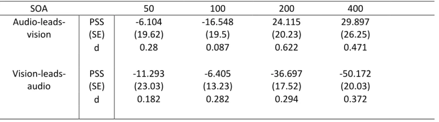
Table 2. PSS, standard error of the mean (SE), and Cohen’s d (d) for comparing PSS when n-1 SOA was audio-leads-vision (first row) against PSS when n-1 SOA was 0 ms and the same for vision-leads-audio (second row). PSS when n-1 SOA was 0 ms was -29.576 (SE = 19.07).
SOA 50 100 200 400 Audio-leads-vision PSS (SE) -6.104 (19.62) -16.548 (19.5) 24.115 (20.23) 29.897 (26.25) d 0.28 0.087 0.622 0.471 Vision-leads-audio PSS (SE) -11.293 (23.03) -6.405 (13.23) -36.697 (17.52) -50.172 (20.03) d 0.182 0.282 0.294 0.372
Figure 2B shows the average PSS for the remaining 18 participants, for trials following each n-1 SOA. As reported above, the difference in effect of n-1 SOA on TOJ PSS is clearly going in the opposite
direction to that reported by Van der Burg and colleagues (2013) for SJ. Consequently, there isn’t much
value in making pairwise predictions for each n-1 SOA combination based on that previous data. Instead, in Table 2. we report the effect size (Cohen’s d) rather than any inferential statistics for each of the n-1 SOA comparisons. Note that the raw data is available in the Supplementary Material for any further exploratory analysis that may be of interest. The pattern of differences is as expected given visual inspection of Figure 1B, with larger effect sizes for comparisons of more distal n-1 SOA (e.g. n-1 SOA audio-leads-vision by 400 ms versus n-1 SOA of 0 ms Cohen’s d = 0.471, while n-1 SOA audio-leads-vision by only 50 ms versus n-1 SOA of 0 ms returns a Cohen’s d of 0.28). In combination with
the statistical comparison reported above for overall n-1 negative versus n-1 positive SOA, these descriptive statistics clearly demonstrate that the effect of previous trials on subsequent judgements
for TOJ is different to that for SJ –unlike for prolonged adaptation, single trial ‘rapid recalibration’
does not produce the same results across different relative timing tasks.
Magnitude Judgements
To retrieve an estimate of PSS from participants’ MJs to compare with the results from SJ and TOJ we
assumed fixed, binary TOJ criterion centred on physical synchrony (0 ms). If the participant reported a value greater than 0 ms, this was taken as a response of ‘vision first’, and if 0 ms or less was reported, this was taken as report of ‘audio first’ (as in Roach et al., 2011). The remaining analysis procedure
was then the same as for real TOJ.
Taking again the hypothesis driven by the results reported by Van der Burg and colleagues (2013) for SJ, we split the data by whether the n-1 trial contained an audio-leads-vision or vision-leads-audio SOA.
Two participants’ data was excluded because their magnitude reports were not proportional to the
physical SOA presented, indicating that they could not discriminate between presented SOAs. Using the same prior given by a half-normal distribution with a mean of 0 and standard deviation in effect size of 0.9295, and with the predicted direction of effect being that PSS for trials where n-1 SOA had been negative would be smaller than when the n-1 SOA had been positive – we conducted a Bayesian paired-samples T-test. As for the TOJ, the results of this test indicated strong evidence against the hypothesis that the PSS for trials where n-1 SOA was negative (mean PSS negative n-1 = 86.805 ms) were smaller than when they follow positive (mean PSS positive n-1 = 43.273 ms) n-1 SOA trials (BF-0 = 0.064). A purely exploratory analysis on the basis of the opposite numerical direction of the effect, a Bayesian T-test with a prior with a mean of 0, effect size of 0.9295, but the opposite predicted direction (PSS n-1 negative SOA > PSS n-1 positive SOA) returned a Bayes Factor of BF+0 = 124.256), extreme evidence for the opposite effect. Again, as this test was not based on any clear motivating hypothesis it should be interpreted with caution.
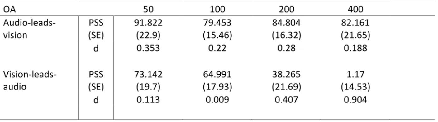
Table 3. PSS, standard error of the mean (SE), and Cohen’s d (d) for comparing PSS when n-1 SOA was audio-leads-vision (first row) against PSS when n-1 SOA was 0 ms and the same for vision-leads-audio (second row). PSS when n-1 SOA was 0 ms was 86.74 (SE = 20.45).
OA 50 100 200 400 Audio-leads-vision PSS (SE) 91.822 (22.9) 79.453 (15.46) 84.804 (16.32) 82.161 (21.65) d 0.353 0.22 0.28 0.188 Vision-leads-audio PSS (SE) 73.142 (19.7) 64.991 (17.93) 38.265 (21.69) 1.17 (14.53) d 0.113 0.009 0.407 0.904
Following the procedure for the analysis above for SJ and TOJ, we then split the data by each n-1 SOA to compare against n-1 SOA of 0 ms. Figure 2C shows the average PSS for 18 participants, for trials following each n-1 SOA. Table 2. shows the effect size (Cohen’s d) each of the n-1 SOA comparisons against n-1 SOA of 0 ms. The pattern of differences is again as expected given visual inspection of Figure 1C, with larger effect sizes for comparisons of more distal n-1 SOA, though only for the vision-leads-audio side (e.g. n-1 SOA vision-vision-leads-audio by 400 ms versus n-1 SOA of 0 ms Cohen’s d = 0.904, while n-1 SOA the vision-leads-audio by only 50 ms versus n-1 SOA of 0 ms returns a Cohen’s d of
0.113). Consistent with the results reported for TOJ, the results for MJ support that serial dependence in relative timing is not the same as prolonged adaptation as the results differ depending on the relative timing task used.
Discussion
Previous studies have shown that repeated exposure, as well as a single exposure, to a specific audiovisual timing relationship produce negative after-effects consistent with sensory adaptation for multisensory relative timing (Linares et al., 2016). While well established that negative after-effects can be found for all relative timing tasks following repeated exposure, only simultaneity judgements have been examined in the case of a single exposure (serial dependence for audiovisual relative timing). Here we investigated whether serial dependence for other common relative timing
judgements - temporal order and magnitude estimation judgements - also produced negative after-effects. If a single audiovisual relative timing exposure is sufficient to produce sensory adaptation, that is, a change the underlying coding of audiovisual relative timing, it would be expected that all relative timing judgements would be affected, regardless of task, as is the case following repeated exposure. While we could replicate negative after-effects in serial dependence for SJ, we found the exact opposite effect when using TOJ and MJ – positive after-effects, like those typically found for serial dependence in other sensory dimensions (e.g. Corbett et al., 2011; Liberman et al., 2014; Fischer & Whitney, 2014; Alais et al., 2015; Taubert et al., 2016a). This task dependency of audiovisual relative timing serial dependence indicates that, unlike repeated exposure, a single exposure does not produce sensory adaptation for audiovisual relative timing.
If serial dependence for relative timing is not the same as sensory adaptation, then the question remains as to why the results of previous studies using SJs have repeatedly found negative after-effects, consistent with those found following repeated exposure. And further, why do the different tasks show different results at all? The answer to both questions might be addressed by considering the different ways in which exposure might affect timing perception, and judgements made on that basis.
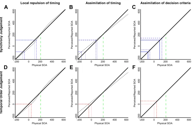
Figure 3. depicts a series of cartoon simplifications of potential effects of exposure on the transduction of physical relative timing into perceptual relative timing, and the related decision criteria. The left column depicts a local repulsion effect on perceptual relative timing such as has been reported following repeated exposure to a specific audiovisual relative timing (Roach et al., 2011; Roseboom et al., 2015). The middle column depicts an assimilation effect on perceptual relative timing such as typically found for serial dependence and described by simple Bayesian decision models (e.g. Petzschner et al., 2015). The right column shows no effect on perceptual relative timing, but an assimilative shift of the decision criteria (for SJ and TOJ) towards the exposed asynchrony, similar to
that previously suggested as an explanation for the effect of repeated relative timing exposure in SJs (Yarrow et al., 2011; 2013; 2015) and for audiovisual synchrony hysteresis (Martin et al., 2015).
Caveats for these descriptions: For simplification, here we consider SJ and TOJ decision criteria to have perfect precision. Consequently, these descriptions don’t include any possible influence of exposure -induced changes in decision criteria precision. Though this is not likely to be the case, the described cases are still informative. These examples use a single stimulus value for relative timing exposure (vision-leads-audio by 200 ms), though the same process could be applied equally to other values of exposure stimulus.
Local repulsion of relative timing
Local repulsion (Figure 3A, 3D) is a change in transduction often associated with sensory adaptation in many sensory dimensions (Webster, 2011; 2016; see Roseboom et al., 2015 and Linares et al., 2016). Here, stimulus values nearby the exposed stimulus are repelled away from it. As can be seen in Figures 3A and 3D, due to the repulsion effect, perception of vision-leads-audio by 100 ms now occurs when a physical value of vision-leads-audio by up to 120 ms is presented (comparing the solid and dashed near diagonal lines, representing pre- and post-exposure relative timing transducers). For SJs (Figure 3A), before exposure, placing decision criteria at perceived +/- 100 ms (solid blue lines) would result in the observer reporting synchrony for physical inputs between audio-leads-vision and vision-leads-audio by 100 ms. Taking the halfway point between these criteria as an estimate of PSS (as done in the above data analyses), the PSS will be around physical synchrony (0 ms). If a participant attempted to maintain the same SJ decision criteria placements after exposure (dashed blue lines), this would lead to physical values up to vision-leads-audio by 120 ms being reported as synchronous on one side of physical synchrony, and physical values up to audio-leads-vision by 80 ms on the other side, producing a PSS shifted in the direction of vision-leads-audio – the direction of the exposed value –
relative to reports made before exposure. This outcome is consistent with known findings for SJ following repeated (Fujisaki et al., 2004) and single (Figure 2A; Van der Burg et al., 2013) exposures.
Figure 3. Different effects of exposure on perceptual transduction of relative timing and their interpretation by synchrony and temporal order judgements. The horizontal axis shows the physical audiovisual relative timing stimulus onset asynchrony (SOA), while the vertical axis shows the transduced, perceived (or reported) SOA. Each panel depicts a different effect of exposure on perceptual relative timing and the associated decision criteria for a SJ or TOJ. In each panel, the vertical long dashed (green) line at 200 indicates the timing of the exposed value (vision-leads-audio by 200 ms in this case). The solid diagonal line indicates the pre-exposure transducer (veridical transduction in this simplified cartoon). In the left and middle columns, the dotted line near diagonal indicates the post-exposure transducer. In the Synchrony Judgement panels (top row), the solid (blue) intersecting vertical and horizontal lines indicate SJ decision criteria placement pre-exposure and the short dashed (blue) lines the placement post-exposure. In the Temporal Order Judgement panels (bottom row), the solid intersecting vertical and horizontal (red) lines indicate the TOJ decision criterion placement pre-exposure and the short dashed (red) lines the placement post-pre-exposure. See text for further description.
For TOJs (Figure 3D), the TOJ criterion placement will be nearby physical synchrony to separate audio- and vision-first temporal orders. Before exposure (solid red lines), this criterion placement will separate audio-leads-vision from vision-leads-audio values, resulting in a PSS of physical synchrony (0 ms). Following the exposure-induced repulsive changes in the transducer, a criterion placement at perceived 0 ms (dashed red lines) will result in values up to vision-leads-audio by 20 ms being reported as audio first, leading to a shift in PSS, again in the direction of the exposed stimulus timing – the opposite of our results for single exposure (Figure 2B), but consistent with previous results following repeated exposure (Vroomen et al., 2004). These descriptions broadly constitute our understanding of what is happening following repeated asynchrony exposure in all tasks (Roach et al., 2011; Roseboom et al., 2015; Linares et al., 2016).
(Bayesian) Assimilation of relative timing
Moving on to the assimilation of timing effects (Figures 3B, 3E), these kinds of effects are consistent with classic regression-to-the-mean effects (Hollingworth, 1910) and have been described by Bayesian decision models wherein a given report is attracted towards prior experience (Petzschner et al., 2015; Linares et al., 2016). Here, reports for stimulus values nearby the exposed stimulus (vision-leads-audio by 200 ms) are assimilated towards it – a flattening of the transducer around the exposed value, with smaller stimulus values reported as larger and larger values as smaller (perfect assimilation would produce a horizontal line such that all physical input values would always be reported as vision-leads-audio by 200 ms in Figures 3B and 3E, for example). Under these changes in transducer, if an observer tried to maintain the same SJ criteria placement before (solid blue lines) and after (dashed blue lines) exposure, the change in the underlying transduction of relative timing would result in a shift in reported synchrony, this time with values between audio-leads-vision by 180 ms and vision-leads-audio by 90 ms being reported as synchronous (by comparison with -100 to +100 ms before). This would lead to a shift in PSS towards audio-leads-vision values, away from the exposed timing and the
opposite of what was found in this study and previously (repeated exposure, Fujisaki et al., 2004; single exposure, Van der Burg et al., 2013) for SJs.
Looking at the assimilation effect in the context of TOJs (Figure 3E), we can see that maintaining a TOJ criterion placement at 0 ms (red lines) while relative timing is assimilated towards the prior (vision-leads-audio by 200 ms in this case) will result in an increase in reports of vision-first for physical audio-leads-vision stimulus timings (difference between solid and dashed red vertical lines in Figure 3E). This change in apparent relative timing would lead to a shift in PSS towards audio-leads-vision values and away from the exposed stimulus timing – the direction of results found for TOJs in our data (Figure 2B). In this interpretation we assume that the assimilation effect is adjusting the reportable values for relative timing. Consequently, this effect will also be seen in the MJ (assimilation effects are commonly dealt with under magnitude estimation or manual reproduction tasks; see Petzschner et al., 2015). As we estimate PSS for MJ by putting that data through a mock TOJ procedure, the process described here for TOJ also applies to, and is therefore consistent with, our results for MJ (Figure 2C). These findings lead to an interesting conclusion regarding the hierarchical architecture of relative timing judgements – rather than being based on a comparator with access to low-level audiovisual timing signals, such as a basic coincidence detector (e.g. Parise & Ernst, 2016), TOJs are based on the output of a relative timing magnitude estimation system, with that system subject to biases generated by Bayesian decision processes.
Assimilation of decision criteria
Looking finally to what happens to the PSS when relative timing transduction is not affected by exposure, but placement of decision criteria is, we consider Figures 3C and 3F. As transduction is unaffected in this case, maintaining criteria placement would not produce any after-effect, contrary to experimental findings. However, if the placement of decision criteria were biased towards the exposed value, in SJs this would lead to a similar shift in PSS as described for repulsive after-effects (again, the difference between the solid and dashed blue lines), with values between
audio-leads-vision by 80 ms to audio-leads-vision-leads-audio by 120 ms being reported as synchronous – producing a shift in PSS towards vision-leads-audio values, and the exposed stimulus timing. Again, this result is consistent with the effect found both in this (Figure 2A) and previous studies for SJs.
For the TOJs, shifting the decision criteria towards the exposed stimulus timing (difference between intersecting solid and dashed red lines) will result in more audio-first reports for vision-leads-audio stimulus values, and therefore a shift in PSS towards vision-leads-audio values – the opposite of the effect we found here, though consistent with the effects of repeated exposure.
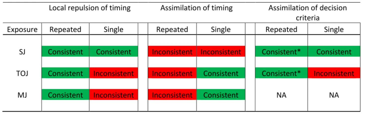
The overall pattern of results from this investigation, indicating which putative changes in relative timing perception or decisions are consistent with the findings both in this study, and those using repeated exposure mentioned in the introduction is shown in Table 4. While the different types of exposure induced changes are presented as distinct, it is possible that one or more are contributing to any given behavioural result. However, there is some evidence that assimilation of decision criteria may not play such a large role in the effects found repeated exposure in SJs* (and possibly TOJs*), as the size of the exposure-induced effect in performance judgments almost perfectly mirrors those reported for appearance judgements (Roseboom et al., 2015). However, no study has yet directly compared the effects of repeated exposure concurrently on appearance and performance tasks.
Table 4. Summary of different effects of exposure and whether they match experimental results reported following repeated or single exposure to asynchrony.
Local repulsion of timing Assimilation of timing Assimilation of decision criteria
Exposure Repeated Single Repeated Single Repeated Single
SJ Consistent Consistent Inconsistent Inconsistent Consistent* Consistent TOJ Consistent Inconsistent Inconsistent Consistent Consistent* Inconsistent
Moreover, to get the complex pattern of changes in reports regarding relative timing appearance and performance that have previously been found following repeated exposure (Roach et al., 2011 for appearance, Roseboom et al., 2015 for performance) would require the complex interplay of many decision criteria (more than the one considered for TOJ and two considered for SJ), making these results often best accounted for by exposure-induced changes in a neural population code representing the range of possible relative timings, rather than shifts in decision criteria (Roach et al., 2011; though see Yarrow et al., 2015 for counter-evidence).
Sensory adaptation and serial dependence in relative timing
Given the information presented thus far, it may be possible to draw a meaningful conclusion regarding the likely processes underlying relative timing after-effects found following repeated and single exposures. As mentioned earlier, if the serial dependence found for SJ was related to sensory adaptation, as is suggested by the negative after-effect, it would be expected that a single exposure would be sufficient to produce negative after-effects in all tasks, as found following repeated exposure. However, this was not the case in our data. In seeking for possible alternative explanations for the negative after-effect in serial dependence of SJs, we find that an assimilation in the decision criteria, like that previously suggested as an account for the effects of repeated exposure (Yarrow et al., 2011; 2013; 2015), may produce the appropriate results. However, such an approach cannot describe our serial dependence results for TOJs and MJs. These results appear consistent with the results often found for serial dependence (positive after-effects) and can likely be accounted for in the same way, using simple Bayesian decision models (Petzschner et al., 2015). This leaves us with an overall picture such that:
− Repeated exposure to a specific relative timing results in negative after-effects, consistent with repulsive neural processes found for sensory adaptation in many sensory dimensions.
− Serial dependence for relative timing in TOJ and MJ is consistent with assimilative effects in relative timing perception and can be accounted for by Bayesian decision models as used in other cases of serial dependence.
− Serial dependence for relative timing in SJ is consistent with assimilative effects in the SJ decision criteria placement, rather than assimilation on the relative timing estimate itself.
Function of after-effects in relative timing perception
The above described configuration of processes and behavioural results facilitates reflection on the functional value of adaptive relative timing perception and serial dependence in general. In many papers (Fujisaki et al., 2004; Vroomen et al., 2004; Vroomen & Keetels, 2010; Van der Burg et al., 2013; Turi et al., 2016; Grabot & van Wassenhove, 2017; Simon et al., 2018) discussing after-effects induced by audiovisual exposure, it has been suggested that the function of these after-effects is to put audio and visual signals in sync, despite the possible differences in transmission and processing latencies (King & Palmer, 1985; Spence & Squire, 2003; King, 2005). Adaptive realignment of physically asynchronous audiovisual inputs would potentially maximise the advantages in perceptual classification (such as identifying the contents of audiovisual speech in noisy environments; Arnold et al., 2010) provided by physically synchronised audiovisual signals. However, this proposed function is at odds with both the generally proposed functions for sensory adaptation, which focus on enhanced neural efficiency and/or improved sensitivity for stimulus values nearby repeatedly exposed stimulus values (Kohn, 2007; Webster, 2011, Webster, 2016), and the mixed results found regarding the relationship between relative timing perception and audiovisual integration (van Wassenhove et al., 2007; Freeman et al., 2013; Harrar et al., 2017; see Linares et al., 2016 for discussion).
By contrast, recent work on serial dependence in the visual domain has cast the role of positive after-effects as to stabilise perceptual experience, by making successive perception(s) apparently more similar (Fischer & Whitney, 2014; Alais, Leung et al., 2017; Kiyonaga, et al., 2017; Fritsche et al., 2017). This kind of explanation is conceptually akin to that previously proposed for audiovisual relative timing
after-effects (maintaining stable perception despite physical variability in input signals) and appears to fit with the results for serial dependence data we found overall (though realised through different processes for TOJ and SJ). It appears that a functional dichotomy wherein rapidly induced positive after-effects that promote perceptual stability (at a cost to perceptual discrimination due to perceptual assimilation making physically different stimuli look more alike), and negative after-effects that emerge over prolonged (repeated) exposure and are related to enhanced neural processing efficiency and perceptual sensitivity, provides a reasonable summary of the potential functional relationship between these behavioural effects. This interpretation is similar to those emerging to describe serial effects in other sensory domains (Bliss et al. 2017; Fritsche et al., 2017; Suárez-Pinilla et al., 2018).
Conclusions
This study has shown that serial dependence for relative timing is not equivalent to the sensory adaptation seen following prolonged exposure, despite apparent similarities in behavioural effects in simultaneity judgements. Our findings suggest that relative timing serial dependence may be better accounted for by a combination of assimilative, positive after-effects, consistent with serial dependence in other perceptual contexts, and described by Bayesian decision models. Differences in serial dependence between relative timing tasks can be accounted for by these assimilation effects acting at different levels of processing and decision making. This account, combined with the previously suggested account for sensory adaptation in relative timing perception, allows us to draw a functional landscape wherein rapid, assimilative changes in perception stabilise perceptual experience, while changes in perception produced by prolonged exposure are related to neural coding efficiency and enhanced perceptual discrimination. This account is broadly consistent with proposals made for serial dependence and sensory adaptation effects across multiple sensory dimensions, suggesting that multisensory relative timing processing operates according to neural and perceptual processes common to many perceptual dimensions.
Acknowledgements
I would like to thank Anil Seth, Daniel Linares, Kielan Yarrow and Virginie van Wassenhove for their assistance and discussions regarding this work. This work was supported by the Dr Mortimer and Theresa Sackler Foundation and the EU FET Proactive grant TIMESTORM: Mind and Time:
References
1. Alais, D., Orchard-Mills, E., Van der Burg, E. (2015). Auditory frequency perception adapts rapidly to the immediate past. Attention, Perception and Psychophysics, 77(3), 896-906. 2. Alais, D., Ho, T., Han, S., Van der Burg, E. (2017). A Matched Comparison Across Three
Different Sensory Pairs of Cross-Modal Temporal Recalibration From Sustained and Transient Adaptation. i-Perception, 8(4). doi: 10.1177/2041669517718697.
3. Alais, D., Leung, J., van der Burg, E. (2017). Linear summation of repulsive and attractive serial dependencies: orientation and motion dependencies sum in motion
perception. Journal of Neuroscience, 37(16), 4381–4390. doi:10.1523/JNEUROSCI.4601-15.2017.
4. Arnold, D.H., Tear, M., Schindel, R. & Roseboom, W. (2010). Audio-Visual Speech Cue Combination. PLoS One, 5(4): e10217.
5. Brainard, D. H. (1997). The Psychophysics Toolbox. Spatial Vision, 10, 433-436. 6. Bliss, D. P., Sun, J. J., D'Esposito, M. (2017). Serial dependence is absent at the time of
perception but increases in visual working memory. Scientific Reports, 7, 1, 14739.
7. Cicchini, G. M., Anobile, G., & Burr, D. C. (2014). Compressive mapping of number to space reflects dynamic encoding mechanisms, not static logarithmic transform. Proceedings of the National Academy of Sciences, 111(21), 7867-7872.
8. Corbett, J.E., Fischer, J., Whitney, D. (2011). Facilitating Stable Representations: Serial Dependence in Vision. PLoS ONE 6(1): e16701.
9. Di Luca, M., Machulla, T.K., & Ernst, M.O. (2009). Recalibration of multisensory simultaneity: cross-modal transfer coincides with a change in perceptual latency. Journal of Vision, 9, 7 1-16.
10. Dienes, Z. (2014). Using Bayes to get the most out of nonsignificant results. Frontiers in Psychology, 5, 781. doi:10.3389/fpsyg.2014.00781
11. Fischer, J., & Whitney, D. (2014). Serial dependence in visual perception. Nature Neuroscience, 17(5), 738-743.
12. Freeman, E.D., Ipser, A., Palmbaha, A., Paunoiu, D., Brown, P., Lambert, C., Leff, A. & Driver, J. (2013). Sight and sound out of synch: Fragmentation and renormalisation of audiovisual integration and subjective timing. Cortex, 49, 2875–2887. doi:10.1016/j.cortex.2013.03.006 13. Fritsche M, Mostert P, de Lange FP. (2017). Opposite Effects of Recent History on Perception
and Decision. Current Biology, 27:1-6. doi:10.1016/j.cub.2017.01.006
14. Fujisaki, W., Shimojo, S., Kashino, M., & Nishida, S. (2004). Recalibration of audiovisual simultaneity. Nature Neuroscience, 7(7), 773–778.
15. Grabot, L. & Virginie van Wassenhove, V. (2017). Time Order as Psychological Bias. Psychological Science, 1–9. DOI: 10.1177/0956797616689369
16. Harrar, V., Laurence R. Harris, L.R. & Spence, C. (2017). Multisensory integration is independent of perceived simultaneity Experimental Brain Research, 235:763–775. DOI:10.1007/s00221-016-4822-2.
17. Hollingworth, H.L. (1910). The central tendency of judgment. Journal of Philosophy, Psychology and Scientific Methods 7(17):461–469.
18. JASP Team (2018). JASP (Version 0.8.3.1)
19. King, A. J. & Palmer, A. R. (1985). Integration of visual and auditory information in bimodal neurones in the guinea-pig superior colliculus. Experimental Brain Research, 60(3), 492–500. doi: 10.1007/BF00236934.
20. King, A.J. (2005). Multisensory integration: strategies for synchronization. Current Biology, 15, R339–341.
21. Kiyonaga, A., Scimeca, J.M., Bliss, D.P, & Whitney, D. (2017). Serial Dependence across Perception, Attention, and Memory. Trends in Cognitive Sciences, 21(7), 493-497.
22. Kleiner, M., Brainard, D., & Pelli, D., 2007, “What’s new in Psychtoolbox-3?” Perception 36
23. Kohn, A. (2007). Visual adaptation: physiology, mechanisms, and functional benefits. Journal of Neurophysiology, 97:3155-3164.
24. Liberman, A., Fischer, J., & Whitney, D. (2014). Serial dependence in the perception of faces. Current Biology, 24(21), 2569–2574.
25. Linares, D., Cos, I., & Roseboom, W. (2016). Adaptation for multisensory relative
timing. Current Opinion in Behavioral Sciences, 8, 35-41. doi:10.1016/j.cobeha.2016.01.005. 26. Machulla, T., Di Luca, M., Froehlich, E., & Ernst, M. O. (2012). Multisensory simultaneity
recalibration: storage of the aftereffect in the absence of counter-evidence. Experimental Brain Research, 217(1), 89-97.
27. Martin, J-R., Kösem, A., & van Wassenhove, V. (2015). Hysteresis in Audiovisual Synchrony Perception. PLoS ONE 10(3): e0119365. doi:10.1371/journal.pone.0119365
28. Michelson, A. A. (1927). Studies In optics. Chicago: University of Chicago Press. 29. Parise, C.V. & Ernst, M.O. (2016). Correlation detection as a general mechanism for
multisensory integration. Nature Communications, 7:11543. doi: 10.1038/ncomms11543. 30. Pelli, D. G. (1997). The VideoToolbox software for visual psychophysics: transforming
numbers into movies. Spatial Vision, 10, 437-442.
31. Petzschner, F.H., Glasauer, S., & Stephan, K.E. (2015). A Bayesian perspective on Magnitude Estimation. Trends in Cognitive Sciences. 19(5):285–293.
32. Roach, N. W., Heron, J., Whitaker, D., & Mcgraw, P.V. (2011). Asynchrony adaptation reveals neural population code for audio-visual timing. Proceedings of the Royal Society of London B: Biological Sciences, 278(1710), 1314– 1322.
33. Roseboom, W., Linares, D., & Nishida, S. Y. (2015). Sensory adaptation for timing perception. Proceedings of the Royal Society of London B: Biological Sciences, 282(1805), 20142833. 34. Rouder, J. N. (2014). Optional stopping: No problem for Bayesians. Psychonomic Bulletin &
35. Schoenbrodt, F. D., Wagenmakers, E.-J., Zehetleitner, M., & Perugini, M. (2015). Sequential hypothesis testing with Bayes factors: Efficiently testing mean differences. Psychological Methods, 22(2), 322-339.
36. Simon, D.M., Nidiffer, A.R. & Wallace, M.T. (2018). Single Trial Plasticity in Evidence
Accumulation Underlies Rapid Recalibration to Asynchronous Audiovisual Speech. Scientific Reports, 8, 12499. doi:10.1038/s41598-018-30414-9.
37. Spence, C., & Squire, S.B. (2003). Multisensory integration: maintaining the perception of synchrony. Current Biology, 13, R519–R521.
38. Suárez-Pinilla, M., Seth, A.K. & Roseboom, W. (2017). Serial dependence in the perception of visual variance. Journal of Vision, 18, 4. doi:10.1167/18.7.4.
39. Taubert J., Van der Burg E., & Alais D. (2016a). Love at second sight: Sequential dependence of facial attractiveness in an on-line dating paradigm. Scientific Reports, 6, 22740.
doi:10.1038/srep22740.
40. Taubert J., Van der Burg E., & Alais D. (2016b). Different coding strategies for the perception of stable and changeable facial attributes. Scientific Reports 6, 32239.
doi:10.1038/srep32239.
41. Turi, M., Karaminis, T., Pellicano, E. & Burr, D. (2016). No rapid audiovisual recalibration in adults on the autism spectrum. Scientific Reports 6, 21756. doi: 10.1038/srep21756. 42. Van der Burg, E., Alais, D., & Cass, J. (2013). Rapid recalibration to audiovisual asynchrony.
Journal of Neuroscience, 33(37), 14633–14637.
43. Van der Burg, E., & Goodbourn, P. T. (2015). Rapid, generalized adaptation to asynchronous audiovisual speech. Proceedings of the Royal Society of London B: Biological Sciences, 282(1804), 20143083–20143083.
44. Vroomen, J., Keetels, M., de Gelder, B., & Bertelson, P. (2004). Recalibration of temporal order perception by exposure to audio-visual asynchrony. Cognitive Brain Research, 22, 32-35.
45. Vroomen, J., & Keetels, M. (2010). Perception of intersensory synchrony: A tutorial review. Attention, Perception, & Psychophysics, 72, 871-884. doi:10.3758/APP.72.4.871. 46. Webster, M.A. (2011). Adaptation and visual coding. Journal of Vision, 11(5):3.
doi:10.1167/11.5.3.
47. Webster, M.A. (2016). Visual adaptation. Annual Review of Vision Science, 1, 547-567. doi: 10.1146/annurev-vision-082114-035509.
48. Yarrow, K., Jahn, N., Durant, S., & Arnold, D.H. (2011). Shifts of criteria or neural timing? The assumptions underlying timing perception studies. Conscious and Cognition. 20, 1518 –
1531.
49. Yarrow, K., Sverdrup-Stueland, I., Roseboom, W. & Arnold D.H. (2013). Sensorimotor temporal recalibration within and across limbs. Journal of Experimental Psychology: Human Perception and Performance, 39(6), 1678-1689.
50. Yarrow, K., Minaei, S., & Arnold, D.H. (2015). A model-based comparison of three theories of audiovisual temporal recalibration. Cognitive Psychology, 83, 54-76.