Zurich Open Repository and Archive University of Zurich Main Library Strickhofstrasse 39 CH-8057 Zurich www.zora.uzh.ch Year: 2015
Continuous on-board monocular-vision-based elevation mapping applied to
autonomous landing of micro aerial vehicles
Forster, Christian ; Faessler, Matthias ; Fontana, Flavio ; Werlberger, Manuel ; Scaramuzza, Davide
Abstract: In this paper, we propose a resource-efficient system for real-time 3D terrain reconstruction and landing-spot detection for micro aerial vehicles. The system runs on an on-board smartphone processor and requires only the input of a single downlooking camera and an inertial measurement unit. We generate a two-dimensional elevation map that is probabilistic, of fixed size, and robot-centric, thus, always covering the area immediately underneath the robot. The elevation map is continuously updated at a rate of 1 Hz with depth maps that are triangulated from multiple views using recursive Bayesian estimation. To highlight the usefulness of the proposed mapping framework for autonomous navigation of micro aerial vehicles, we successfully demonstrate fully autonomous landing including landing-spot detection in real-world experiments.
DOI: https://doi.org/10.1109/ICRA.2015.7138988
Posted at the Zurich Open Repository and Archive, University of Zurich ZORA URL: https://doi.org/10.5167/uzh-110753
Conference or Workshop Item Published Version
Originally published at:
Forster, Christian; Faessler, Matthias; Fontana, Flavio; Werlberger, Manuel; Scaramuzza, Davide (2015). Continuous on-board monocular-vision-based elevation mapping applied to autonomous landing of micro aerial vehicles. In: IEEE International Conference on Robotics and Automation (ICRA), Seattle WA, 26 May 2015 - 30 May 2015, 111-118.
Continuous On-Board Monocular-Vision–based Elevation Mapping
Applied to Autonomous Landing of Micro Aerial Vehicles
Christian Forster, Matthias Faessler, Flavio Fontana, Manuel Werlberger, Davide Scaramuzza
Abstract— In this paper, we propose a resource-efficient system for real-time 3D terrain reconstruction and landing-spot detection for micro aerial vehicles. The system runs on an on-board smartphone processor and requires only the input of a single downlooking camera and an inertial measurement unit. We generate a two-dimensional elevation map that is prob-abilistic, of fixed size, and robot-centric, thus, always covering the area immediately underneath the robot. The elevation map is continuously updated at a rate of 1 Hz with depth maps that are triangulated from multiple views using recursive Bayesian estimation. To highlight the usefulness of the proposed mapping framework for autonomous navigation of micro aerial vehicles, we successfully demonstrate fully autonomous landing including landing-spot detection in real-world experiments.
MULTIMEDIAMATERIAL
A video attachment to this work is available at:
http://rpg.ifi.uzh.ch
I. INTRODUCTION
Autonomous Micro Aerial Vehicles (MAVs) will soon play a major role in industrial inspection, agriculture, search and rescue and consumer goods delivery. For autonomous operations in these fields, it is crucial that the vehicle is at all times fully aware of the surface immediately underneath: First, during normal operation, the vehicle should maintain a minimum distance to the ground surface to avoid crashing. Second, for autonomous landing, the MAV needs to identify, approach and land at a safe site without human interven-tion. Knowing the ground surface in previously-unknown environments is invaluable in case of forced landings due to emergencies like communication loss as well as for planned landings for, e.g., saving energy during monitoring operations or for the delivery of goods.
Large-scale Unmanned Aerial Vehicles (UAVs) often use range sensors to detect hazards, avoid obstacles or to land autonomously [1], [2]. However, these active sensors are expensive, heavy and quickly drain the battery when used on small MAVs. Instead, given efficient and robust computer vision algorithms, active range sensors can be replaced by a single downward-looking camera. This setup is lightweight, cost effective, and, as shown in previous works [3], allows accurate localization and stabilization of the MAV in GPS denied environments, such as indoors, close to buildings, or below bridges.
The authors are with the Robotics and Perception Group, University of Zurich, Switzerland—http://rpg.ifi.uzh.ch. This research was supported by the Swiss National Science Foundation through project number 200021-143607 (“Swarm of Flying Cameras”) and the National Centre of Competence in Research Robotics (NCCR).
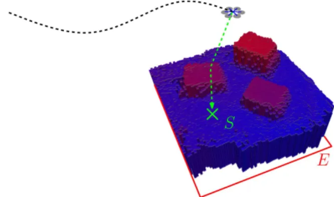
Fig. 1: Illustration of the local elevation map E. The two-dimensional probabilistic grid map is of fixed size and centered below the MAV’s position. The MAV updates the map continuously at a rate of 1 Hz using only the on-board smartphone processor and data from a single down-looking camera. The map enables the robot to autonomously detect and approach a landing spotSat any time (green trajectory).
In contrast to stereo and RGBD-cameras with fixed base-lines, a single moving camera may be seen as a stereo setting that can dynamically adjust its baseline according to the required measurement accuracy as well as the structure and texture of the scene. Indeed, a single moving camera represents the most general setting for stereo vision. This property was previously exploited for real-time 3D terrain reconstruction from aerial images in order to detect landing spots [4]–[6] or for visualization purposes [7]–[10].
In this paper, we propose a system for mapping the local ground environment underneath an MAV equipped with a single camera. Detailed dense and textured reconstructions are valuable for human operators and can be computed in real-time but off-board by streaming images to a ground station as shown in [8]–[10]. In order to work also for emergency maneuvers or autonomous flying in remote areas without the availability of a ground station, we restrict the system to solely use the computing capability on-board the MAV. To achieve this objective we utilize a coarse two-dimensional elevation map [11] as on-board map represen-tation, which is sufficient for many autonomous maneuvers in outdoor environments. A further advantage compared to other map representations, such as surface meshes [7], is the regular sampling of the surface and the possibility to fuse multiple elevation measurements via a probabilistic representation. The proposed system runs continuously on an on-board smartphone processor and updates the robot-centric elevation map of fixed dimension at a rate of 1 Hz. The system does not require any prior information of the scene or external navigation aids such as GPS.
A. Related Work
Real-time dense reconstruction with a single camera has been previously demonstrated in [8], [9], [12]–[14]. How-ever, all previous approaches rely on heavy GPU paralleliza-tion and therefore can currently not be computed with the on-board computing power of an MAV. In [9] we presented the REMODE (regularized monocular depth estimation) al-gorithm and demonstrated live but off-board dense mapping from an MAV. Therefore, we streamed on-board pose es-timates provided by an accurate visual odometry algorithm [15] together with images at a rate of 10 Hz to a ground station that was equipped with a powerful laptop computer and was capable to compute dense depth maps in real-time. In the current paper, we utilize REMODE to build a 2D elevation map and present modifications to the algorithm to run it on a smartphone CPU on-board the MAV.
Early works on vision-based autonomous landing for Unmanned Aerial Vehicles (UAV) were based on detecting known planar shapes (e.g., helipads with “H” markings) in images [16] or on the analysis of textures in single images [17]. Later works (e.g., [4]–[6]) assessed the risk of a landing spot by evaluating the roughness and inclination of the surface using 3D terrain reconstruction from images.
The first demonstration of vision based autonomous land-ing in unknown and hazardous terrain is described in [4]. Similar to our work, structure-from-motion was used to estimate the relative pose of two monocular images and subsequently, a dense elevation map with a resolution of19×
27 cells was computed by matching and triangulating 600 regularly sampled features. The evaluation of the roughness and slope of the computed terrain map resulted in a binary classification of safe and hazardous landing areas. While this work detects the landing spot entirely based on two selected images, we continuously make depth measurements and fuse them in a local elevation map.
In [5], homography estimation was used to compute the motion of the camera as well as to recover planar surfaces in the scene. Similar to our work, a probabilistic two-dimensional grid was used as map representation. However, the grid stored the probability of the cells being flat and not the actual elevation value as in our approach, therefore, barring the possibility to use the map for obstacle avoidance. While previously mentioned works were passive in the sense that the exploration flight was pre-programmed, recent work [6] wasactivelychoosing the best trajectory to explore and verify a landing spot. Due to computational complexity, the full system could not run entirely on-board in real-time. Thus, outdoor experiments were processed on datasets. In contrast to our work, only two frames were used to compute dense motion stereo, hence a criterion, based on the visibility of features and the inter-frame baseline, was needed to select two images. The probabilistic depth estimation in our work not only allows using every image for robust incremental estimation but also provides a measure of uncertainty that can be used for planning trajectories minimizing the uncertainty as fast as possible [18].
Visual Odometry (SVO)
Sensor Fusion (MSF) On-board computer
IMU Camera
Dense Depth Estimation (REMODE-CPU)
pose
scaled & gravity aligned pose 50 Hz 200 Hz 10 Hz Elevation Map depth map, 1 Hz MAV Control Path Planning mission
Fig. 2: Overview of the main components and connections in the proposed system. All modules are running on-board the MAV.
B. Contributions
The contribution of this work is a monocular-vision– based 3D terrain scanning system that runs in real-time and continuously on a smartphone processor on-board an MAV. Therefore, we introduce a novel robot-centric elevation map representation to the MAV research community. To highlight the usefulness of the proposed elevation map, we demonstrate both indoor and outdoor experiments of a fully integrated landing spot detection and autonomous landing system for a lightweight quadrotor.
II. SYSTEMOVERVIEW
Figure 2 illustrates the proposed systems’ main compo-nents and their linkage:
We use our Semi-direct Visual Odometry (SVO) [15] to estimate the current MAV’s pose given the image stream from the single downward-looking camera.1 However, with a single camera we can obtain the relative camera motion only up to an unknown scale factor.
Therefore, in order to align the pose correctly with the gravity vector, and to estimate the scale of the trajectory, we fuse the output of SVO with the data coming from the on-board inertial measurement unit (IMU). For integrating the IMU’s data, we use the MSF (multi-sensor fusion)software package [19], which utilizes an extended Kalman filter.2
Next, we compute depth estimates with a modified version of the REMODE (REgularized MOnocular Depth Estimation)
[9] algorithm. Details on the modifications of the REMODE algorithm for computing probabilistic depth maps purely relying on the on-board computing capability are given in Section III.
The generated depth maps are then used to incrementally update a 2D robot-centric elevation map [11]. Since the elevation map is probabilistic, we perform a Bayesian update step for the elevation values of the affected cells, whenever a new depth map is available. In addition, the elevation
1Available athttp://github.com/uzh-rpg/rpg_svo 2Available athttps://github.com/ethz-asl/ethzasl_msf
Initialize Depth Filters
REMODE-CPU
SVO Image & Pose
pose yes Regularize New Reference Frame? Update Depth Filters no Converged? yes Depthmap sparse depth no next frame
Fig. 3: Overview of the monocular dense reconstruction system.
map moves together with the robot’s pose as it is local and robot-centric. More details on the update steps and how to incorporate the depth measurements are given in Section IV. The flight trajectory of the MAV is provided by the path planning module which can be implemented in different ways: For instance, it has a pre-programmed flight path, or it obtains way-points from a remote operator, or it uses active vision in order to select the next-best views to make the current depth map converge as fast as possible. For further details on the active vision approach, we refer to [18].
As an exemplar application of the given system, we show an autonomous landing of the MAV. Therefore, an additional module forlanding-spot detectionbased on the elevation map is presented in Section V.
III. MONOCULARDENSERECONSTRUCTION
In the following, we summarize the REMODE (REgu-larized MOnocular Depth Estimation) algorithm, which we introduced in [9], and describe the necessary modifications to run the algorithm in real-time on a smartphone processor on-board the MAV.
An overview of the algorithm is given in Figure 3. The algorithm computes a dense depth map for selected reference views. The depth computation for a single pixel is formalized as a Bayesian estimation problem. Therefore, a so called
depth filteris initialized for all pixels in every newly selected reference imageIr (see Figure 4). Every subsequent image Ikis used to perform a recursive Bayesian update step of the
depth estimates. The selection of reference frames — hence the amount of generated depth maps given a sequence of images — is based on two criterions: a new reference view is selected whenever (1) the uncertainties of the given depth estimates are below a certain threshold (thus the depth map has converged), or (2) when the spatial distance between the current camera pose and the reference view is larger than a certain threshold. After the depth map converged, we enforce its smoothness by applying a Total Variation (TV) based image filter.
A. Depth Filter
Given a new reference frameIr, a depth filter is initialized
for every pixel with a high uncertainty in depth and a mean that is derived from the sparse 3D reconstruction in the visual
Trk Ir Ik ˆ di ui u ′ i ˜ dk i dmini dmaxi l T r World W
Fig. 4: Probabilistic depth estimatedˆifor pixeliin the reference framer.
The point at the true depth projects to similar image regions in both images (blue squares). Thus, the depth estimate is updated with the triangulated depth d˜k
i computed from the point u′i of highest correlation with the
reference patch. The point of highest correlation lies always on the epipolar line in the new image.
odometry (see Section III-C). The depth filter is described by a parametric model that is updated on the basis of every subsequent frame k.
Let the rigid body transformationTWr∈SE(3)describe
the pose of a reference framer relative to the world frame W. Given a new observation {Ik,TWk}, we project the
95% depth-confidence interval[dmin
i , dmaxi ]of the depth filter
corresponding to pixel i into the image Ik and find a
segment of the epipolar line l (see Figure 4). Using the zero-mean sum of squared differences (ZMSSD) score on a 8×8 patch, we search the pixel u′
i on the epipolar line
segment l that has highest correlation with the reference pixel ui. A depth measurement d˜ki is generated from the
observation by triangulating ui and u′i from the views r
andk respectively. As proposed in [20], we can model the measurements with a model that mixes “good” measurements (i.e., inliers) with “bad” ones (i.e., outliers). With probability
ρi, the measurement is a good one and is normally distributed
around the correct depth di with a measurement variance τk
i
2
. With probability 1−ρi, the measurement is an outlier
and is uniformly distributed in an interval[dmin i , dmaxi ]): p( ˜dk i|di, ρi) =ρiN( ˜dki|di, τik 2 ) + (1−ρi)U( ˜dki|d min i , d max i ), (1)
Assuming independent observations, the Bayesian estimation fordion the basis of all measurementsd˜ri+1, . . . ,d˜
k i is given by the posterior p(di, ρi|d˜ri+1, . . . ,d˜ k i)∝p0(di, ρi) Y k p( ˜dk i|di, ρi), (2)
withp0(di, ρi)being a prior on the true depth and the ratio
of good measurements supporting it. A sequential update is implemented by using the estimation at time stepk−1as a prior to combine with the observation at time stepk. We refer to [20] for the final formalization and in-depth discussion of the update step.
Note that we consider the depth estimate that is modeled as a Gaussiandi∼ N( ˆdi,σˆ2i)as converged when its estimated
inlier probabilityρˆi is more than the thresholdηinlierand the
depth varianceσˆ2
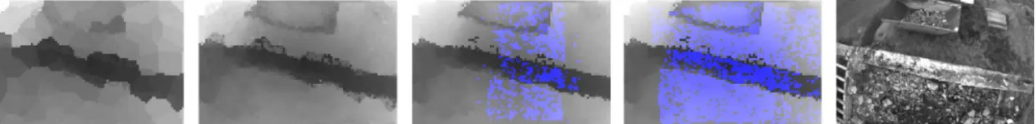
Fig. 5: Evolution of the depth map reconstruction process. The leftmost image shows the depth map after initialization from the sparse point cloud. After some iterations, the depth filters converge upon which their corresponding pixels are colored in blue. The final depth map is integrated in the elevation map shown in Figure 8(b). The rightmost image shows the reference image of the depth map.
B. Depth Smoothing
The main goal is to filter coarse outliers in the depth estimate but keep the discontinuities in the depth map intact. In [9], we utilized a variant of the weighted total variation, introduced by [21] in the context of image segmentation, in order to enforce spatial smoothness of the constructed depth maps. Therefore, we utilize the given depth mapD(u)with
u ∈ R2 being the image coordinates. For computing the smooth depth mapF(u), we apply a variant of the weighted Huber-L1 model as presented in [9], that is defined as the variational problem min F Z Ω G(u)k∇F(u)kε+λ(u)kF(u)−D(u)k1 du. (3)
Note that there are two modifications to the variant presented in [9]: (1) first, we use a weighted Huber regularizer that weights the Huber norm according to the image gradient magnitude of the respective reference image by using the weighting function G(u) = exp −α||∇Ir(u)|| q 2 . (4)
This is based on the assumption that image edges of the reference image coincide with depth discontinuities, hence prevents the regularization to smooth across object bound-aries. (2) Second, we define λ(u), the trade-off between regularization and data fidelity, as a pointwise function depending on the estimated pixel-wise depth uncertainty ˆ
σ2(u)and inlier probability ρˆ(u)of the depth filters:
λ(u) =E[ˆρ(u)]σ 2 max−σˆ2(u) σ2 max , (5) whereσ2
max is the maximal uncertainty that the depth filters
are initialized with. The confidence value λ(u) represents the quality of the convergence of the depth value for each pixel. In the extreme case, if the expected value of the inlier probabilityρˆ(u)is zero or the variance is close toσ2
max, the
confidence value λ(u) becomes zero and solving (3) will perform inpainting for these regions.
For solving the optimization problem (3), we refer to [9] where we defined the primal-dual formulation of the weighted Huber-L1 model. Then, for solving such dual saddle-point problems we utilize the first-order primal-dual algorithm proposed by Chambolle and Pock [22].
C. Implementation Details
On-board the MAV, only a coarse elevation map is nec-essary for autonomous maneuvers. This requirement allows us to lower the resolution of the reconstruction, which drastically reduces the processing time for one depth map.
In practice, we initialize one depth filter for every 8×8 pixel block in the reference frame. We therefore obtain dense depth maps of size 94×60, totalling 5820 depth filters for every reference image. Given the computing capabilities of our platform, we can update the depth filters in real-time; thus, we do not require to buffer any images and provide frequent updates to the elevation map.
More accurate initialization of the depth filters further reduced the processing time. Hence, we exploit that the visual odometry algorithm already computes a sparse point-cloud of the scene (shown in Figure 9(b)). We create a two-dimensional KD-Tree of the sparse depth estimates in the reference frame and find for every depth-filter the closest sparse depth estimate. The result is a mosaic of locally-constant depths as shown in the leftmost image of Figure 5. In case a depth estimate is very close to the depth-filter, the initial depth uncertaintyσˆ2i is additionally reduced for faster
convergence. This approach relies on the fact that SVO has few outliers. However, in case of an outlier, we find that the depth-filters do not converge and, thus, no erroneous height measurement will be inserted in the elevation map. In Figure 5, converged depths are colored in blue and from visual inspection it can be seen that most obvious outliers have not converged. Resulting holes in the elevation map are quickly filled by subsequent updates.
IV. ELEVATIONMAP
We make use of a recently developed robot-centric eleva-tion mapping framework proposed in [11]. The goal of the original work was to develop a local map representation that serves foot-step planning for walking robots over and around obstacles. However, we find that the local two-dimensional elevation map is an efficient on-board map representation for MAVs that are flying outdoors — it allows us to keep a safe distance to the surface and to detect and approach suitable landing spots. By tightly coupling the local map to the robot’s pose, the framework can efficiently deal with drift in the pose estimate. The local map has a fixed size, thus, the map can be implemented with a two-dimensional circular buffer that requires constant memory. The two-dimensional buffer allows moving the map efficiently together with the robot without copying any data but by shifting indices and by resetting the values in the regions that move out of the map region. An open-source implementation of the elevation mapping framework is provided by the authors of [11].3
While the authors of [11] used a depth camera, we will demonstrate how the elevation map can be efficiently updated
p rf
T
hWorld
Map
Camera
d u Ir Cell (i, j) WCT
MCFig. 6: Notation and coordinate frames used for the elevation map.
with depth maps computed from aerial monocular views. Furthermore, we extended the framework with a system to switch the map resolution – a requirement that is necessary when the MAV is operating at different altitudes.
A. Preliminaries
We use three coordinate frames, the inertial world frame W is assumed fix, the map frame M is attached to the elevation map, and C denotes the camera frame attached to the MAV (see Figure 6). Since the elevation map is robot centric, the translation part of the rigid body transformation
TMC(t) ={RMC(t),MtMC} ∈SE(3)remains fixed at all times. The MAV has an onboard vision-based state estimator that estimates the relative transformationTWC(t)∈SE(3).
The elevation map is stored in a two-dimensional grid with a resolutions[m/cell]and widthw[m]. The height in each cell (i, j) is modeled as a normal distribution with mean ˆh
and varianceσˆ2
h. B. Map Update
In Section III, we described how to process data from a single camera to obtain a probabilistic depth estimate d ∼ N( ˆd,ˆσ2
d)corresponding to a pixeluin a selected reference
image Ir, where r = C(tr) denotes the camera frame C
at a selected time instant tr. Given the probabilistic depth
estimate, we can follow the derivation in [11] to integrate a measurement in the elevation map. In the following, we summarize the required steps.
Given the depth estimate dˆof pixel u, we can find the corresponding 3D pointpby applying the camera model:
Cp¯ =π
−1(u)·d,ˆ
(6) whereπ−1 is the inverse camera projection model that can be obtained through camera calibration. The prescript c
denotes that the pointcp¯is expressed in the camera frame of
reference and the bar indicates that the point is expressed in homogeneous coordinates. We find the height measurement by transforming the point to map coordinates and applying the projection matrixP= [0 0 1]that maps a 3D point to a scalar value:
˜
h=P TMC Cp¯. (7)
To obtain the variance of the measurement, we need to compute the Jacobian of the projection function (7):
JP=
∂˜h ∂Cp
=P RMC, (8)
where RMC ∈ SO(3) is the rotational part of TMC. The variance of the measurement can then be written as:
˜
σ2h=JPΣpJ⊤P. (9)
Note that Equation (9) can be extended with the uncertainty corresponding to the robot poseTCW as derived in [11]. The uncertainty of the 3D pointΣp is derived as follows:
Σp=Rdiag( ˆ d fσ 2 p, ˆ d fσ 2 p, σ 2 d)R ⊤ , (10)
where R is a rotation matrix that aligns the pixel bearing vector f with the z-axis of the camera coordinate frame C. The fraction dˆ
f projects the pixel uncertaintyσ
2
p (set fixed to
one pixel) to the 3D space, using the focal length f of the camera.
Given the height measurement meanh˜ and variance σ˜2
h,
we can update the height estimate in the corresponding cell (i, j)using a recursive Bayesian update step:
ˆ h← σ˜ 2 hˆh+ ˆσ2hh˜ ˜ σ2 h+ ˆσ 2 h , σˆ2h← ˜ σ2 hσˆ2h ˜ σ2 h+ ˆσ 2 h . (11) C. Map-Resolution Switching
Given the height z of the robot above ground in meters, the focal lengthf in pixels, and the fact that we initialize a depth-filter for every image block of 8 pixels size, we can compute the optimal elevation map resolution:
sopt=
8
f ·z [m/cell]. (12)
For instance, when flying at a height of 5 meters with our camera that has a focal length f = 420pixels, the optimal resolution would be0.1 meters per cell. We limit the size of the map to have 100 by 100 cells; thus, depending on the resolution, a larger or smaller area is covered by the elevation map.
During operation, we maintain an estimate of the optimal resolutionsopt and compare it with the currently-set
resolu-tionscur. If the MAV is ascending and the optimal resolution
increases by a factor αup = 1.8 compared to the current
resolution, we double the resolution. Similarly, if the optimal resolution reduces by a factor ofαdown= 0.6, i.e., the MAV
is approaching the surface, we reduce the resolution by half. Additionally, we limit the minimal resolution to 5 cm per cell to avoid changing the resolution too often during the landing procedure. When the resolution changes, we down or up-sample all values in the map using bilinear interpolation.
V. LANDINGSPOTDETECTION
To motivate the usefulness of the proposed local elevation map, we implemented a basic landing-spot detection and landing system that is described in the following.
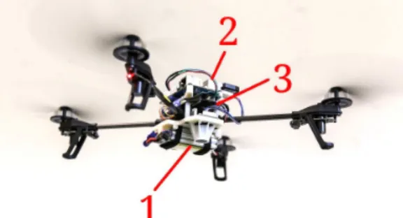
Fig. 7: Experimental platform with (1) down-looking camera, (2) on-board computer, and (3) inertial measurement unit.
Let us define a 3D point plocated on the surface of the terrain and within the range of the local elevation map. The point has discrete coordinates (i, j)in the two-dimensional elevation map and is located at heighth(i, j).
We define a safe landing spot to have a local neighborhood of radiusrin which the surface is flat. The radiusris related to the size of the MAV. We formalize this criterion with the cost function:
C(i, j) = X
(u,v)∈R(i,j,r)
||h(u, v)−h(i, j)||2, (13)
where R(i, j, r) is the set of cells around coordinate (i, j) that are located within a radius r.
Experimentally, we find a thresholdCmax that defines the
acceptable cost to be a safe landing spot. We compute a binary mask of all cells in the elevation mask, which have a cost lower thanCmax. Subsequently, we apply the distance
transform to the binary mask in order to find the coordinates (i, j)that have a cost lower than the threshold and are farthest from all cells that do not satisfy the criterion. Thus, the final landing spot should be as far as possible from any obstacles. From the construction of the elevation map, it may well be that a cell does not have an elevation value. This is the case in regions that have not been measured before or in which the depth filters did not converge, e.g., due to lack of texture, reflections, or due to moving objects. Therefore, before applying the kernel in Equation (13) to the elevation map, we set all cells without an elevation value to Cmax.
Thereby, assuring to land in regions where depth computation is feasible, thus, landing is more likely to be safe.
VI. EXPERIMENTS
We performed experiments of the elevation-mapping and landing system both indoors in a quadrotor testbed as well as outdoors. Videos of the experiments can be viewed at:
http://rpg.ifi.uzh.ch
The quadrotor used for all experiments is shown in Fig-ure 7. It is equipped with a MatrixVision mvBlueFOX-MLC200w752×480-pixel monochrome global shutter cam-era, an 1.7 GHz quad-core smartphone processor running Ubuntu, and an PX4FMU autopilot board from Pixhawk that houses an Inertial Measurement Unit (IMU). In total the quadrotor weights less than 450 grams and has a frame diameter of 35 cm. More details about the experimental platform are given in [10].
Mean Median Std. Dev. [ms] [ms] [ms] Depthmap update 150 143 40 Regularization (10 iterations) 133 129 19 Elevation map update 10 10 2 Total time for one depthmap: 1098 999 503 Landing spot detection 268 268 19
TABLE I: On-board timing measurements. A. Timing Measurements
All processing during the experiments was done on the on-board computer using the ROS4 middleware. During
operation, the elevation-mapping and landing module uses, on average, one processing core, SVO and MSF together another two cores, and the fourth core is reserved for the camera driver, communication, and control.
Table I lists the timing measurements. On average, the depth map requires 6 to 10 images for convergence. However, this depends greatly on the motion of the camera as well as the depth and the texture of the scene [18]. For the listed measurements, we were flying at a speed of approximately 1.5 m/s and at a height of 1.8 meters. Updating all depth estimates with a new image requires on average 150 millisec-onds. Once 50% of the depth filters in the depth map have converged, we filter the resultand depth map by solving the gradient-weighted Huber-L1 model (3) (130 milliseconds) and integrate the smoothed depth map in the elevation map (10 milliseconds).
Summarizing, the mapping module receives images from the camera at 10 Hz and integrates approximately 6-10 images to output one depth map per second.
Once it is necessary to detect a landing spot, it requires approximately 268 milliseconds to compute the landing cost (13) for all 10,000 grid cells and to find the best landing-spot in the current elevation map.
B. Outdoor mapping experiment
For the outdoor elevation-mapping experiment, the quadrotor was commanded by a remote operator under assistance of the on-board vision-based controller, i.e., the operator could command the quadrotor directly in x-y-z-yaw space. On average, the quadrotor was flying 4-5 meters above the surface and used an elevation map of size 10 by 10 meters with a resolution of 10 centimeters per cell. The terrain consisted of a teared-down house, rubble, asphalt, and grass. Figure 8(a) gives an overview of the scenario and indicates the location of the MAV for the elevation maps shown in Figures 8(b) to 8(d). The complete mapping process can be viewed in the video attachment of this work.
An update rate of 1 Hz is sufficient to always maintain a dense elevation map below the MAV. However, when moving in a straight line, the local elevation map behind the MAV is more populated than in the front. In the future, we will modify the MAV to have a slightly forward facing camera in order to have a more even distribution.
The system can cope with drastic elevation changes as well as challenging surfaces such as grass and asphalt that are characterized by high-frequency texture. Due to the probabilistic approach to depth estimation, which uses mul-tiple measurements until convergence, we observe very few outliers in the elevation map. Note that we only insert depth estimates in the elevation map that have actually converged. In untextured regions, paths with of dynamic motion or zones with reflecting surfaces, such as water, the depth filter does not converge and, thus, the elevation map remains empty. As visible in Figure 8(b), the elevation map remains also empty in occluded areas.
C. Landing experiment
We performed autonomous landing experiments both in-doors and outin-doors as demonstrated in the supplemental video. Figure 9(a) shows the indoor testbed that contains textured boxes as artificial obstacles. The elevation map after a short exploration is displayed in Figure 9(b). Once the MAV receives a command to land autonomously, it computes the landing score for the current elevation map and selects the best spot as described in Section V. In Figure 9(c), the elevation map is colored with the landing cost that is formalized in Equation (13). Blue means that the area is flat and, thus, safe for landing. The algorithm selects the point that is farthest from any dangerous area (colored red) and marks it with a green cube. The MAV then autonomously approaches a way-point vertically above the detected landing spot and then slowly descends until vision-based tracking is lost, which is typically at less than 30 cm above ground. Subsequently, the MAV continues blindly to descend until impact is detected and the motors turn off.
VII. CONCLUSION
In this paper, we proposed a system for mapping the local ground environment underneath an MAV using only a single camera and on-board processing resources. We advocate the use of a local, robot-centric, and two-dimensional elevation map since it is efficient to compute on-board, ideal to accumulate measurements from different observations, and is less affected by drifting pose estimates. The elevation map is updated at a rate of 1 Hz with probabilistic depth maps computed from multiple monocular views. The probabilistic approach results in precise elevation estimates with very few outliers even for challenging surfaces with high frequency texture, e.g., asphalt. To highlight the usefulness of the proposed mapping system, we successfully demonstrated autonomous landing-spot detection and landing.
REFERENCES
[1] A. Johnson, A. Klumpp, J. Collier, and A. Wolf, “Lidar-based hazard avoidance for safe landing on mars,”AIAA Jour. Guidance, Control and Dynamics, vol. 25, no. 5, 2002.
[2] S. Scherer, L. J. Chamberlain, and S. Singh, “Autonomous landing at unprepared sites by a full-scale helicopter,”Journal of Robotics and Autonomous Systems, September 2012.
[3] D. Scaramuzza, M. Achtelik, L. Doitsidis, F. Fraundorfer, E. Kos-matopoulos, A. Martinelli, M. Achtelik, M. Chli, S. Chatzichristofis, L. Kneip, D. Gurdan, L. Heng, G. Lee, S. Lynen, L. Meier, M. Polle-feys, A. Renzaglia, R. Siegwart, J. Stumpf, P. Tanskanen, C. Troiani, and S. Weiss, “Vision-Controlled Micro Flying Robots: from System Design to Autonomous Navigation and Mapping in GPS-denied En-vironments,”IEEE Robotics Automation Magazine, 2014.
[4] A. Johnson, J. Montgomery, and L. Matthies, “Vision guided landing of an autonomous helicopter in hazardous terrain,” inIEEE Intl. Conf. on Robotics and Automation (ICRA), 2005.
[5] S. Bosch, S. Lacroix, and F. Caballero, “Autonomous detection of safe landing areas for an uav from monocular images,” inIEEE/RSJ Intl. Conf. on Intelligent Robots and Systems (IROS), 2006.
[6] V. Desaraju, N. Michael, M. Humenberger, R. Brockers, S. Weiss, and L. Matthies, “Vision-based landing site evaluation and trajectory generation toward rooftop landing,” inRobotics: Science and Systems (RSS), 2014.
[7] S. Weiss, M. Achtelik, L. Kneip, D. Scaramuzza, and R. Siegwart, “In-tuitive 3D maps for MAV terrain exploration and obstacle avoidance,”
Journal of Intelligent and Robotic Systems, vol. 61, pp. 473–493, 2011. [8] A. Wendel, M. Maurer, G. Graber, T. Pock, and H. Bischof, “Dense reconstruction onthefly,” in Proc. IEEE Int. Conf. Computer Vision and Pattern Recognition, 2012.
[9] M. Pizzoli, C. Forster, and D. Scaramuzza, “REMODE: Probabilistic, Monocular Dense Reconstruction in Real Time,” inIEEE Intl. Conf. on Robotics and Automation (ICRA), 2014.
[10] M. Faessler, F. Fontana, C. Forster, E. Mueggler, M. Pizzoli, and D. Scaramuzza, “Autonomous, vision-based flight and live dense 3D mapping with a quadrotor MAV,”J. of Field Robotics, 2015. [11] P. Fankhauser, M. Bloesch, C. Gehring, M. Hutter, and R. Siegwart,
“Robot-centric elevation mapping with uncertainty estimates,” in In-ternational Conference on Climbing and Walking Robots (CLAWAR), 2014.
[12] D. Gallup, J.-M. Frahm, P. Mordohai, Q. Yang, and M. Pollefeys, “Real-time plane-sweeping stereo with multiple sweeping directions,” in Proc. IEEE Int. Conf. Computer Vision and Pattern Recognition, 2007.
[13] J. Stuehmer, S. Gumhold, and D. Cremers, “Real-time dense geometry from a handheld camera,” inDAGM Symposium on Pattern Recogni-tion, 2010, pp. 11–20.
[14] R. A. Newcombe, S. Lovegrove, and A. J. Davison, “DTAM: Dense tracking and mapping in real-time,” inIntl. Conf. on Computer Vision (ICCV), 2011, pp. 2320–2327.
[15] C. Forster, M. Pizzoli, and D. Scaramuzza, “SVO: Fast Semi-Direct Monocular Visual Odometry,” in IEEE Intl. Conf. on Robotics and Automation (ICRA), 2014.
[16] S. Saripalli, J. F. Montgomery, and G. S. Sukhatme, “Vision-based autonomous landing of an unmanned aerial vehicle,” in IEEE Intl. Conf. on Robotics and Automation (ICRA), 2002.
[17] P. J. Garcia-Pardo, G. S. Sukhatme, and J. F. Montgomery, “Towards vision-based safe landing for an autonomous helicopter,”Journal of Robotics and Autonomous Systems, vol. 38, 2002.
[18] C. Forster, M. Pizzoli, and D. Scaramuzza, “Appearance-based active, monocular, dense depth estimation for micro aerial vehicles,” in
Robotics: Science and Systems (RSS), 2014.
[19] S. Lynen, M. Achtelik, S. Weiss, M. Chli, and R. Siegwart, “A robust and modular multi-sensor fusion approach applied to mav navigation,” in IEEE/RSJ Intl. Conf. on Intelligent Robots and Systems (IROS), 2013.
[20] G. Vogiatzis and C. Hern´andez, “Video-based, Real-Time Multi View Stereo,”Image and Vision Computing, vol. 29, no. 7, 2011. [21] X. Bresson, S. Esedoglu, P. Vandergheynst, J.-P. Thiran, and S. Osher,
“Fast global minimization of the active contour/snake model,”Journal of Mathematical Imaging and Vision, vol. 28, no. 2, 2007.
[22] A. Chambolle and T. Pock, “A first-order primal-dual algorithm for convex problems with applications to imaging,”Journal of Mathemat-ical Imaging and Vision, vol. 40, no. 1, 2011.
(a) Scenario overview
(b) Viewpoint 1
(c) Viewpoint 2
(d) Viewpoint 3
Fig. 8: Excerpts from the video attachment. The quadrotor is flying over a destroyed building. Figures 8(b) to 8(d) show the elevation map at three different times. The corresponding viewpoints are marked in the scenario overview in Figure 8(a). Note that the elevation map is local and of fixed size. Its center lies always below the quadrotor’s current position.
(a) Scenario
(b) Elevation map
(c) Landing procedure
Fig. 9: Excerpts from the video attachment. Figure 9(a) shows the indoor flying arena with textured obstacles. The MAV first explores the arena and creates an elevation map of the surface that is shown in Figure 9(b). The pink points illustrate the sparse map built by the on-board visual odometry system and which are used to initialize dense depth estimation. Figure 9(c) shows the detected landing spot that is marked as green cube and the MAV that is shortly before impact. The blue line is the trajectory that the MAV flew to approach the landing spot.