Machine Learning for Closure Models in Multiphase-Flow Applications

(1)

Department of Applied Physics

Machine Learning for Closure Models in

Multiphase-Flow Applications

Master Thesis

J.F.H. Buist

Supervisors

ir. Y. van Halder

dr.ir. B. Sanderse

prof.dr.ir. B. Koren

prof.dr.ir. G.J.F. van Heijst

Report Number

R-1959-A

(2)

(3)

Abstract

Multiphase flows are described by the multiphase Navier-Stokes equations. Numerically solving these equations is computationally expensive, and performing many simulations for the purpose of design, optimization and uncertainty quantification is often prohibitively expensive. A cheaper, simplified model, the so-called two-fluid model, can be derived from a spatial averaging process. The averaging process introduces a closure problem, which is represented by unknown friction terms in the two-fluid model. Correctly modeling these friction terms is a long-standing problem in two-fluid model development.

In this work we take a new approach, and learn the closure terms in the two-fluid model from a set of unsteady high-fidelity simulations conducted with the open source code Gerris. These form the training data for a neural network (NN). The NN provides a functional relation between the two-fluid model’s resolved quantities and the closure terms, which are added as source terms to the two-fluid model. With the addition of the locally defined interfacial slope as an input to the closure terms, the trained two-fluid model reproduces the dynamic behavior of high fidelity simulations better than the two-fluid model using a conventional set of closure terms.

High fidelity model

h

u w M = 1 M = 0 g

Neural network

Training data

Closure terms

∂hint ∂s

..

.

uL hint

..

.

..

.

τint τG τL

Low fidelity model

H

uL uG τG τint τL hint g

(4)

(5)

Preface

This thesis was submitted in partial fulfillment of the requirements for the degree of Master of Science in Applied Physics from the Eindhoven University of Technology. The work presented in this thesis was carried out in the Scientific Computing research group of the Centrum Wiskunde & Informatica (CWI) in Amsterdam. Here, I encountered an environment which challenged me to push my boundaries, and dive into new things at every corner of my broad research topic.

I am indebted to my daily supervisors at CWI, Yous van Halder and Benjamin Sanderse. I want to thank Yous for the introduction to multiphase flow CFD, and the engaging discussions on neural networks and new things to try with them. Benjamin I thank for his careful look at my work, his sharp and detailed feedback, and good suggestions for further steps in the project.

Thank you to my supervisor Barry Koren, from the Scientific Computing research group of the department of Applied Mathematics at the Eindhoven University of Technology, for introducing me to CWI. Thank you also for the talks on the way back from Cascade, and your engagement with my project and my future.

My supervisor GertJan van Heijst, from the Turbulence and Vortex Dynamics research group of the department of Applied Physics at the Eindhoven University of Technology, I thank for the critical questions on the physical aspects of my work. Thank you for taking on this new and different topic, and keeping it in line with the requirements for a degree in physics.

Jurriaan Buist

(6)

(7)

Introduction

1.1 Multiphase flow

Gas-liquid multiphase flow is a problem of interest in the oil and gas industry. For example, oil and gas are often transported together in long pipelines from remote fields to an offshore platform or an onshore plant [1]. Ever more remote and deep underwater fields are being tapped as more easily accessible fields are depleted. Transport of liquefied natural gas (LNG) is another hot topic in the oil and gas industry; it is currently greatly on the rise [2], [3]. During the loading and unloading of a carrier, the carrier will be only partially filled with liquid1 _{so that external waves may induce sloshing inside the carrier [2]. This in}

turn may induce harmful rolling motion of the ship [4] or damage the thermal insulation [5].

For these multiphase flows, accurate numerical models have been proposed [6], [7]. However, a trade-off will always have to be made between model accuracy and computational expense. This difficult trade-off has persisted to today.

Some applications require the numerical model to be solved repeatedly. An example isUncertainty Quantification (UQ), which has become an active area of research in recent years. This field (see e.g. [8])

is concerned with determining the effect of model error or input parameter variation on the outcome of the simulation. Different algorithms exist with varying requirements on the number of model evaluations.

Another example where repeated model evaluations are required are optimization problems. Often, in order to find the optimal values of a set of performance indicators, it is desired to calculate these for different values of a potentially large set of tunable parameters. Only with a large number of model evaluations can one map all the local and global minima or maxima in the performance reliably.

For these problems where many potentially expensive model evaluations are required, it is necessary to resort to low fidelity models. These make a trade-off between accuracy and computational efficiency that leans more towards computational efficiency. In this thesis we will study low-fidelity models for the multiphase applications mentioned above.

1.2 Low fidelity model for two-phase pipe flow

One way to create a cheaper model is to reduce the dimensionality of the model. In the case of pipe flow, we are mainly interested in variation of the averaged flow properties along the pipe’s axial direction. We therefore reduce a full three-dimensional (3D) model to a one-dimensional (1D) model. However, the effect of the flow structure in the cross-sectional plane - which the 1D model does not solve for - on the 1D flow variables, must be modeled in some way. We add so-calledclosure terms to the 1D model which approximate this effect. A different well-known example of closure terms is the concept of a turbulence closure model, which models the effect of unresolved turbulence on the averaged flow.

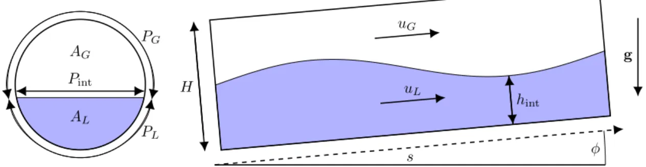
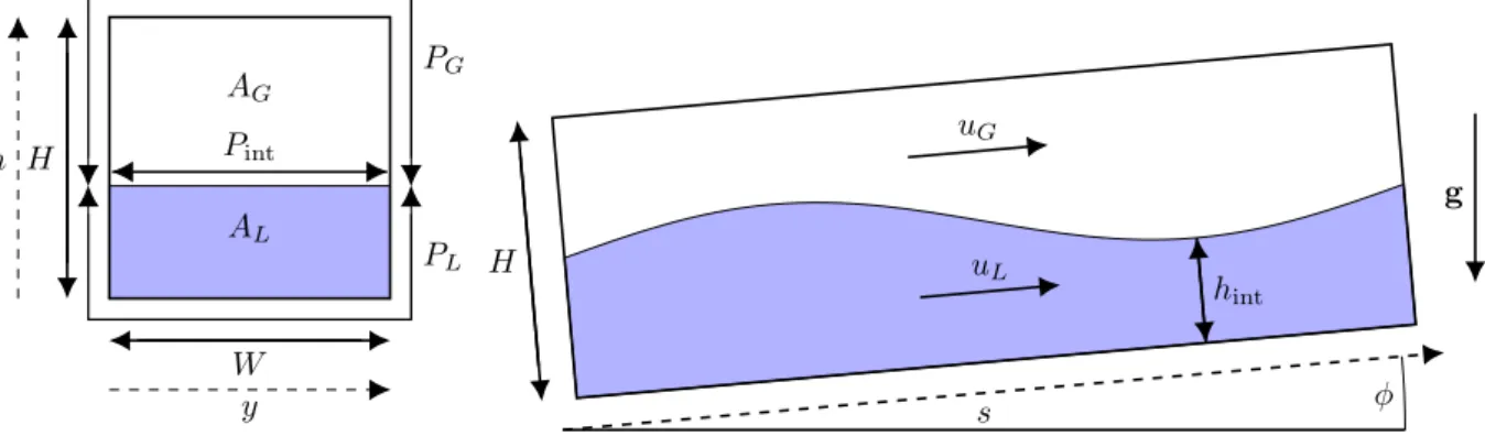
The focus in this project is the 1D stratified two-fluid model, a simplified model for stratified liquid-gas flow in a pipe or square cross-section duct geometry (Figure 1.1). In the 1D two-fluid model the velocity fields are not resolved along the direction normal to the duct wall; they only vary along the direction of flow through the duct (sin the figure). The wall and interface stresses, which are important terms in

1_{In order to liquefy the natural gas, so that it takes up less volume, it is cooled to low temperatures. Due to imperfect}

thermal insulation some of the LNG will evaporate and remain in the tank as a gas phase. Loading and unloading of a carrier may take up to 24 hours, at an offshore platform or at an onshore facility.

(10)

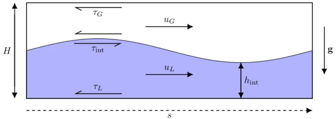
the governing equations, depend on the unresolved wall-normal velocity profile slope. Therefore the 1D two-fluid model requires closure terms for the wall and interface stresses.

AL AG PL PG Pint H uL uG τG τint τL hint g s

Figure 1.1: A schematic of the 1D two-fluid model for a circular pipe. Left: a cross-section, representing a single cell for which the areasAL, AGand the velocitiesuL,uGare defined. Right: a string of these cells together forming a length of the pipe. The total friction terms are calculated as products of the mean stressesτL,τG,τint

and the perimeters over which they act.

For laminar single-phase flow, analytical closure relations are easily found (based on fully developed steady state flow). For turbulent single-phase flow these cannot be found and conventionally closure relations based on empirical data are used, of which a multitude exists (see section 3.4). They are mostly determined for a circular pipe geometry, but this equivalence is not exact and the error is large for the laminar case. The friction factors are usually determined for steady, fully developed flow. They all have a specific range of Reynolds numbers for which they are said to hold. The functional forms of common friction factors are not very insightful; they are simply fit to match data.

For two-phase flow empirical relations are harder to construct because the pressure drop in fully developed flow is now determined by the sum of three different stresses, instead of a single stress in the case of single-phase flow. Additionally, the interfacial stress is complicated to model; depending on the relative fluid viscosities the interface may be approximated as a free surface for the liquid and as a no-slip wall for the gas. The effect of interfacial waves on the interfacial stress is hard to quantify. Furthermore, the possibility of backflow in inclined pipes complicates the situation. The same average velocity may result from a very different flow profile with very different velocity gradients (even reversed), so that expressing the friction closure terms as a function merely of the average velocity becomes dubious, and a correction is hard to find empirically. Additionally, the vast majority of the literature concerns circular pipe flow and it can be hard to find good closure terms for a different geometry.

For two-phase laminar flow, analytical closure relations may be found [9]. In a 2D channel geometry elegant exact expressions are the result, but for pipe flow the expressions are not practical; they require numerical integration of complex integrals. It is great that these analytical solutions exist, but they hold only for steady state, fully developed, smoothly stratified (not wavy) flow.

In conclusion, modeling wall and interface stresses in terms of resolved quantities (averaged velocity fields), either by fitting experimental data or physical arguments, is a difficult task. Our proposed alternative is to the extract friction factors to close the 1D two-fluid model from high-fidelity simulation data. If we have highly resolved 2D or 3D simulation data, the wall and interface stresses can be calculated exactly. From this one can determine a closure relation relating the wall and interface stresses to the averaged flow variables whichare resolved in the two-fluid model. The flow need not be steady state and fully developed; this operation is possible in any kind of flow conditions. With a simulation code the geometry, fluid properties, and initial conditions can be adjusted relatively easily. This would have the advantage of enabling friction factor calculation more specific to the geometry and flow parameters of interest to the user of the two-fluid code. More generally this approach can be useful for the closure of other low fidelity flow models; it was pioneered by Ma et al. [10], [11] for bubbly vertical channel flow.

Different strategies can be conceived for the determination of the closure relations from high fidelity simulation data. A straightforward approach is to use linear regression. Using this approach we would have to assume a functional relation for the closure term, of which the unknown coefficients could be fitted to the data. Having to choose a functional relation could be an advantage, since in defining it we can use our knowledge of the physics of the problem. However, it could also be a disadvantage, since we are in fact already determining the form of the solution, while the data might suggest a different functional form.

(11)

1.3 Neural networks 3 High fidelity model data Neural network Closure term function Low fidelity model

feed to generates apply in

Figure 1.2: The general idea, applicable not only to the low fidelity 1D two-fluid model but to any low fidelity flow model requiring closure.

Therefore we propose to use instead artificial neural networks (ANN) to perform the fitting. The general approach is summarized in Figure 1.2. Using a neural network, we need only to specify a network architecture. The network training algorithm automatically finds a (possibly complex nonlinear) function which fits the data well.

1.3 Neural networks

Artificial neural networks have made a name for themselves in recent years through remarkable results in applications such as image classification [12], natural language processing [13], and learning to beat the masters at the complex Chinese chess-like game of ‘Go’ [14]. This diversity of applications illustrates their remarkable ability to represent complex relations between arbitrary inputs and outputs. Training a neural network is a form of function fitting, but with a complex nonlinear structure which allows the neural network to approximate a wide range of functions2_.

An artificial neural network is a computational graph of connected nodes, which individually perform straightforward operations. They generally take a weighted sum of the values of the incoming connections and apply some non-linear activation function to this sum. The original incarnation of these nodes was called the ‘perceptron’, by researchers who were trying to model the human brain [16]. The power of neural networks lies in the concept of connecting these nodes in large and diverse networks, in ways which model the network of neurons in the brain. A schematic of a simple (fully connected, feed-forward, non-convolutional) network structure is shown in Figure 1.3. The schematic shows one possible structure; the number of hidden layers and number of nodes in each layer can be chosen freely (besides more imaginative alterations).

Essential to their utility is their ability to be trained efficiently, via the backpropagation algorithm [17]. A loss function defined at the output layer measures the current predictive performance of the network for a given set of inputs, by comparing the difference between output training data and the model output. The backpropagation algorithm efficiently calculates the gradient of this loss function to the weights of the node connections, which are the free parameters of the network which determine the degree to which

Input Layer Hidden Layers Output Layer

Figure 1.3: A schematic of a neural network.

2_{A neural network with a single hidden layer can approximate almost any function with an arbitrary degree of accuracy,}

(12)

a signal is passed on between two consecutive nodes. Using this gradient an optimization algorithm can tune the weights; this is called the ‘training’ or ‘learning’ of the network, in analogy to the brain.

Some recent introductions to neural networks are given by [18], [19]. An older book (1996 first edition) by the authors of the MATLAB shallow neural network implementation is [20].

1.4 Neural networks in fluid dynamics

As noted above, the need for closure terms for the shear stresses in 1D flow is analogous to the need for turbulence closure terms in insufficiently resolved turbulent flow. Neural networks have already been applied successfully in this area. Sargini et al. [21] used a neural network to create a subgrid scale (SGS) model for a Large Eddy Simulation (LES), which reproduces the dynamics of LES using an expensive SGS model (Bardina’s scale similar (BFR) SGS model), at a lower computational cost. Their neural network output a turbulent viscosity coefficient (a.k.a. eddy viscosity) as a function of the gradients of the spatially averaged velocities, and products of the velocity fluctuations. Their learned closure term produced good results, for Reynolds numbers within and close to the range of Reynolds numbers used in the training data. Moreau et al. [22] used neural networks fed by pseudospectral DNS data of turbulent flow to model the subgrid variance in the concentration of an advected species for an LES, but did not test simulations with the learned closure term. An eddy viscosity coefficient for atmospheric flow over an urban boundary layer was obtained using a neural network by Esau [23].

Yarlanki et al. [24] tried an unusual inverse approach. The parameters of thek−turbulence model are to be determined and form the inputs to an ANN, and the differences between CFD results and experimental results are the outputs of the neural network. The neural network learns the error between simulation and experiment as a function of the turbulence model parameters, and thus the parameter set which yields the smallest error can be found indirectly. The foundk−model parameters reduced the discrepancy between simulation and experiment significantly compared to standard parameters, for their specific test case. Tracey et al. [25] reproduced the Spalart-Allmaras turbulence closure model (without a specified functional form) from the output of simulations done with this closure model. They report very promising results, but stress the importance of choosing appropriate ANN inputs and cost function. Gamahara and Hattori [26] recently used DNS to obtain a functional relation for the Reynolds stress tensor directly, which shows performance close to that of a Smagorinsky SGS model.

In multiphase flow applications, the use of neural networks to identify closure terms is still in its infancy. One existing example is Lu et al. [27], [28], who trained a neural network with data from micro-scale DNS simulations of a gas-solid mixture under influence of a shock, to provide closure relations for the particle-particle and gas-particle interactions for use in coarse macro-scale simulations. The main inspiration for the current project is taken from Ma et al. [10], [11]. They consider dispersed liquid-gas flow, for which they take a reduced order model, averaged along the streamwise direction and one spanwise direction, and bounded by periodic boundaries in their 3D DNS simulations. The closure relations required for their simplified model are for the wall-normal liquid flux, the average of the product of the streamwise and wall-normal velocities, and the average surface tension. They obtain these using neural networks fed by their 3D DNS data, with good results. They also tried linear regression with a predetermined functional relation, which produced similar results to the neural network, but is deemed by them to be a far less general approach. Gibou et al. [29] review numerical methods for simulating multiphase flow and machine learning applied to computational physics. Their review confirms that there is only limited existing work connecting neural networks and multiphase flow, and raises a number of questions to be tackled.

There has been some work connecting pipe flow stress closure terms (in the form of friction factors) and neural networks. Neural networks were trained to replicate different implicit empirical friction factor correlations by [30]–[38]. For the studies which generate an explicit form of the Colebrook-White friction factor equation (see section 3.4), the inputs are the Reynolds number and the relative roughness and the output is the friction factor. The training data consists of iterative solutions of the Colebrook-White equation for different Reynolds numbers and relative roughnesses. The usefulness of this work is limited though, since simpler explicit approximations of the Colebrook-White equation with a smaller error than the deviation of the Colebrook-White equation from the empirical data have existed for some time (e.g. Haaland (1983) [39]).

(13)

1.5 Project plan 5

more than just a fit of the data, i.e. if their output can incorporate known physical principles. This is a challenging and outstanding problem, but one good illustration of this principle was given by Ling et al. [40]. They remarked that any scalar flow variable, such as pressure or velocity magnitude, will be invariant to rotations, reflections, or translations of the frame of reference. Without special care a machine learning algorithm output will not adhere to this perfectly. Ling et al. describe two ways to enforce rotational invariance on trained neural network outputs in the context of turbulence modelling. One way is to simply feed the neural network training data to which a number of different rotations have been applied. But a far more efficient way is to use as inputs to the neural network only quantities which are themselves rotationally invariant. Doing this naturally ensures that the output is rotationally invariant. Another strategy they employ is making the inputs non-dimensional. This ensures that the output is non-dimensional as well, so that if an output variable is chosen that should indeed be non-dimensional, there will be no problems of dimension in the output functional relation.

Overall, good results are reported in the literature on fluid dynamics with neural networks. In the range of the training data nonlinear relations are reproduced accurately, and simulations using learned closure terms produce results close to the original data. Currently the advantage of neural networks lies in their application to specific cases, to which they may be applied relatively easily to learn correlations specific to a certain set of conditions. However, their extrapolating qualities are still limited, and improvements in choice of network inputs and structure are needed if neural networks to one day outperform e.g. conventional closure terms in general cases.

Particularly in turbulence closure models neural networks have been applied successfully. In multiphase flow the first steps have been made, but the approach is still new, especially for the two-fluid model that we consider in this work. When training neural networks to produce closure terms many difficult choices and trade-offs have to be made, and a lot of work is left to be done before the level of the highly problem-specifically optimized convolutional neural networks such as those used in image classification [12] is reached.

1.5 Project plan

It was discussed in section 1.2 that existing friction closure terms for 1D two-phase flow are lacking. Cases for which analytical solutions cannot be found are usually closed by experiment. But conclusive empirical relations are hard to find in some cases. Therefore in this project the neural network approach to finding closure terms will be applied to this problem. We will train a neural network on high-fidelity computational model data. With this method, the aim of this project is to combine the easy general applicability and accuracy of a high fidelity model with the low computational cost of a simplified model. This would alleviate the existing necessity for trade-offs between accuracy and computational efficiency in the simulation of multiphase flow.

Figure 1.4 shows a schematic of the project plan. We restrict ourselves to (periodic boundary) laminar stratified channel flow, but the plan is applicable to circular pipe flow with some modifications. The figure shows two cases that are discussed in this work: smooth, fully developed, steady state flow and wavy, transient flow. High fidelity simulations can be conducted for both cases with the open-source code Gerris [6], which solves the full viscous incompressible Navier-Stokes equations. We start with smooth, fully developed, steady state channel flow, for which analytical solutions and closure relations are available for channel geometries (see section 3.4). These relations can be used to assess the accuracy of the high fidelity model simulations. Furthermore, we will train neural networks on steady state data and compare this to the analytical closure relations, so that the neural network can be tuned and the approach validated.

For wavy, transient flow, existing closure relations are lacking, and we will proceed to directly train a neural network based on the high-fidelity simulation results, with the same architecture that will have already been validated for the case mentioned above. The new closure terms can be validated by plugging them into the 1D two-fluid code (our low fidelity model) and evaluating if with these closure terms its behavior is similar to the 2D ’truth’ given by the high fidelity model.

(14)

Viscous Navier-Stokes Smooth, fully developed, steady state High-fidelity simulations Stress closure terms Analytical solution as function of body forces Stress closure terms Wavy, transient High-fidelity simulations Stress closure terms Low-fidelity simulations neural network [3] derive [1] validate [2] validate [4] neural network [5] compare [6] validate [8] feed closure [7]

Figure 1.4: A flow chart of the project structure. We analyze two different sets of solutions of the Navier-Stokes equations, one of which has analytical solutions. These are used to validate the high-fidelity (Gerris) simulations and the extraction of closure terms using a neural network. Afterwards the same architecture is applied to construct closure terms for wavy, transient flow, which are then tested in a low-fidelity model.

1.6 Structure of the report

In chapter 2 we outline the physics of stratified multiphase flow, and our high fidelity computational model which we use to model these physics. Chapter 3 presents the 1D stratified two-fluid model and casts it into a form specialized to 2D channel flow. This chapter includes a detailed discussion of the closure terms for the wall and interface stresses and existing empirical relations for them.

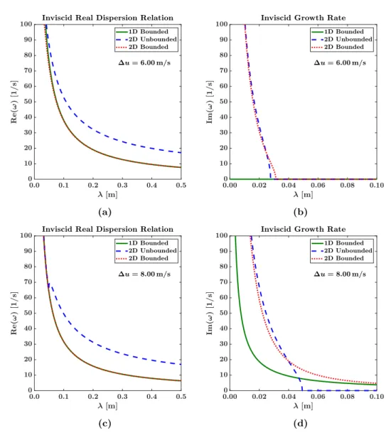
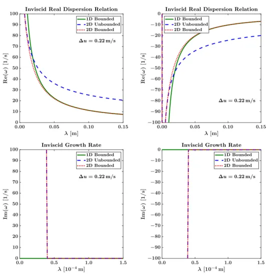
In chapter 4, we analyze the stability and well-posedness of our flow problem. The employed two-fluid model turns out to only be well-posed under certain conditions. A linear stability analysis of the two-fluid model and of a 2D model for the same flow problem yields predictions for the propagation and amplification of small wave-like disturbances. These predictions are used to validate our computational models for the inviscid case, and to examine fundamental restrictions in getting the 1D model to emulate the dynamics of the 2D model. The inviscid dispersion relations may be used for qualitative explanations of phenomena occurring in viscous simulations in later chapters.

In chapter 5 we validate our high and low fidelity models for smoothly stratified (non-wavy) viscous flow. We discuss the difficulties in extracting the required training data for our neural network.

Chapter 6 provides a brief introduction to neural networks, before applying them to the case of fully developed, steady, laminar 2D channel flow. We discuss the choices made in defining our neural network and validate them using the analytical closure terms. Finally, we apply our neural network to the case of wavy, unsteady flow in chapter 7. We test our learned closure terms in the 1D two-fluid model.

(15)

Chapter 2

2D and 3D Multiphase Flow Models

2.1 Introduction

In this chapter we will discuss the physics and solution scheme of our high-fidelity multiphase flow model, which resolves the flow in two or three spatial dimensions. We will first go over the physical laws of fluid dynamics, paying special attention to their application to multiphase flow. These laws form the basis of our computational model. Afterwards we will see a method for solving the equations corresponding to these physical laws on a computational grid. We use the open source code Gerris [6], [41] as our high-fidelity model.

2.2 The Navier-Stokes equations for fluid flows

In the following, we employ the continuum hypothesis. This means averaging out individual interacting molecules into a continuous fluid with continuously defined properties such asρ(density) andu(velocity). This allows us to convert the principles of mass and momentum conservation into a set of continuous equations; the Navier-Stokes equations. See also textbooks such as [42], [43].

2.2.1 Mass conservation

In any classical1 physical system, mass must be conserved. This means that the change in time of the mass inside a control volumeV, illustrated in Figure 2.1, is equal to the mass flowing in and out of the control volume at its boundaries. For the flow of a continuous fluid this can be written as

d dt Z V ρdV =− I S ρu·ndS, (2.1)

where d/dtis a derivative with respect to time,R

VdV is an integral over the control volumeV,ρ=ρ(x, t)

is the density (xrepresenting coordinates in three-dimensional space andtrepresenting time),H SdS is

an integral over the closed surfaceS boundingV, u=u(x, t) is the velocity vector and·nis the inner product with the vector normal to the surfaceS, pointing outward.

Since the control volume V is fixed in space, the time derivative on the left hand side can be brought inside the integral using Leibniz’ rule. For the right hand side we can apply the divergence theorem, or Gauss’ theorem, to obtain

Z V dρ dt dV =− Z V ∇·(ρu) dV. (2.2)

In the limitV →0 the above implies

∂ρ

∂t +∇·(ρu) = 0. (2.3)

This is a specific form of the generic conservation law ∂q

∂t +∇·f(q) =c(q), (2.4)

(16)

s h S0 S1 n1 n1 n0 n0 n1 n0 n1 n0 V0 V1 u w g

Figure 2.1: A schematic of two control volumes V0,V1 in two-phase flow. The control volumes are bounded

byS0 andS1respectively, with normal vectors pointing outward. Here we place the boundaries of the control

volumes on the interface so that they only ever contain one fluid. The spatial coordinate vectorxhas components

s,y(not pictured), andh. The velocities in these directions are the componentsu,v, andwofu, respectively.

where q=q(x, t) is a conserved quantity,f is the flux of qandc is a source of q(which can also be a function ofq).

In (2.3) the flux is only the convective flux of ρ

fC =ρu. (2.5)

If there are multiple species, there may also be a diffusive flux, given by Fick’s law, with a diffusion coefficientD:

fi=fC,i+fD,i, with fC,i=ρiu, fD,i=D∇ρi. (2.6)

In our model the flux is only the convective flux, since we make theassumption of sharp interfaces [44, p. 22]. The fluids are assumed immiscible, so they do not diffuse into each other. Then a change ofρin the control volume can only result from a net flow of mass, i.e. (2.5).

The material derivative describes the change of a property of a fluid parcel as we follow it during its flow. It can be defined

D Dt =

∂

∂t+u· ∇(). (2.7)

Using this and an expansion of the divergence operator:

∇·(ρu) =u·∇ρ+ρ∇·u, (2.8)

(2.3) can be rewritten as

Dρ

Dt =−ρ∇·u. (2.9)

This shows that the density of a fluid parcel can only change if the flow is divergent or convergent, in which case the fluid parcel expands or compresses. The flow can be said to be incompressible if this does not happen:

∇·u= 0, (2.10)

in which case the density of a fluid parcel traveling with the flow does not change. Though in the incompressible case a fluid parcel cannot be compressed or expanded, the density might still vary between different fluid parcels (e.g. between two different fluids in a multiphase flow simulation).

(17)

2.2 The Navier-Stokes equations for fluid flows 9

2.2.2 Momentum conservation

Momentum conservation for fluids is an application of Newton’s second law. The change in time of the momentum contained in a control volume is dictated by the magnitude and direction of the forces acting upon it. Momentum can also enter or leave the control volume with the flow, just as mass can. These ideas can be expressed mathematically as

d dt Z V ρudV =− I S ρu(u·n) dS− I S pndS+ I S τ·ndS+ Z V ρgdV, (2.11)

wherep=p(x, t) is the pressure,τ =τ(x, t) is the stress tensor, andgis the gravity force vector. For any fixed control volume V this equation will hold so that via Gauss’ theorem and Leibniz’s rule the differential form

∂ρu

∂t =−∇·(ρuu)−∇p+∇·τ+ρg (2.12)

can be found, where

∇·(ρuu) =ρu·∇u+u∇·(ρu), (2.13)

so that using (2.3) the balance is reduced to

ρ∂u

∂t +ρu·∇u=−∇p+∇·τ+ρg. (2.14)

On the left hand side we can now recognize the material derivative ofu(multiplied byρ). The intermediate form (2.12) is an equation in conservative form (2.4), withq=ρu,

f =fC+fD, with fC=ρuu, fD=−τ, (2.15)

and

c=ρg−∇p. (2.16)

In this interpretation,ρuu is the convective flux of momentum, the stress term represents diffusion of momentum, and the pressure gradient and gravitational field are sources of momentum.

The interpretation of −τ as a diffusive flux of momentum is justified by its constitutive law for Newtonian fluids τ = 2µ D−1 3(∇·u)I +ζ(∇·u)I, (2.17)

withIthe identity matrix andDthe rate of strain deformation tensor. According to Stokes’ hypothesis the bulk viscosityζis zero. If furthermore incompressibility is assumed, the stress tensor reduces to

τ = 2µD, (2.18)

where D = 1₂ ∇u+∇uT

and in Cartesian coordinates, with x = (s, y, h) and u = (u, v, w) (see Figure 2.1), andDis given by

D=    ∂u ∂s 1 2( ∂v ∂s+ ∂u ∂y) 1 2( ∂w ∂s + ∂u ∂h) 1 2( ∂v ∂s+ ∂u ∂y) ∂v ∂y 1 2( ∂w ∂y + ∂v ∂h) 1 2( ∂w ∂s + ∂u ∂h) 1 2( ∂w ∂y + ∂v ∂h) ∂w ∂h   . (2.19)

For incompressible flow with constant density and viscosity, by substitution of∇·u= 0 andµ=ρν, it can be shown that

∇·τ =∇·ρν

∇u+ (∇u)T

=ν∇2_ρ_u₌_∇_·_ν_∇_ρ_u_. _(2.20)

Thus, returning to (2.4) and (2.15), for all intents and purposes we could writefD=−τ =−ν∇ρu. This

is exactly Fick’s form of the diffusive flux (given in (2.6) for mass), but with the kinematic viscosityν playing the role of diffusion coefficient.

(18)

2.2.3 Energy conservation

A similar expression as for mass and momentum conservation can be formulated for energy conservation. Alternatively, the flow can be assumed isothermal, and the system can be closed with an equation of state

ρ=f(p). (2.21)

This eliminates the need for an energy equation.

For incompressible flows neither an energy equation nor an equation of state is needed. The density is determined by

Dρ

Dt = 0, (2.22)

as discussed in subsection 2.2.1. If a fluid starts out with uniform density, then in an incompressible flow the fluid will retain that density everywhere and (2.22) need not be solved.

The pressure must be such that it forces, via the momentum balance, the velocity to satisfy (2.10). The pressure is the only unknown besides the velocity in the momentum balance (2.14). With these multiple unknowns there are multiple combinations ofuandpwhich satisfy the momentum balance. But the continuity equation (2.10) narrows the choice down to one possible combination. If we choose an appropriate pressure, then from the momentum balance we will obtain a velocity field that is incompressible. This can be viewed as the pressure projecting the velocity field into the space of functions that satisfy (2.10) [44].

2.3 Multiphase flow and the interface

The main difficulty in simulating multiphase flow lies in handling the interface. In this project, we deal with two fluids which, as stated before, are immiscible and have a sharp interface. These two fluids may be for example a liquid and a gas. The equations of motion as derived above apply to both fluids separately. They can in principle be solved for one of the fluids at a time, with the influence of the other fluid entering via the boundary conditions at the interface. In practice this can be complicated since the interface is part of the solution and can assume complex forms.

2.3.1 Kinematic boundary conditions

We consider a thin control volume centered on the interface between two fluids, illustrated in Figure 2.2. The thickness of the control volume tends to zero, so that no mass can accumulate inside of it. The control volume travels with the interface at velocityuint. The integral formulation for mass conservation

(2.1) then leads to the Rankine-Hugoniot condition

ρ1(u1−uint)·n=ρ0(u0−uint)·n= ˙m, (2.23)

in whichuint is the interface velocity,u1is the velocity of fluid 1,u0 is the velocity of fluid 0 and ˙mis

the mass flow across the interface. A mass flow across the interface means that one phase gains mass at the expense of the other, and thus implies phase change. If there is no phase change, ˙m= 0.

If there is no phase change, (2.23) leads to the boundary condition

uint·n=u1·n=u0·n, (2.24)

which can also be applied at a solid boundary.

With the continuum hypothesis, there can be no slip between gas and liquid at the interface since a discontinuous velocity profile would result in infinite stress. The no-slip boundary condition can be combined with (2.24) to yield

u1=u0. (2.25)

We can obtain another boundary condition by applying the integral momentum balance (2.11) to the control volume in Figure 2.2. Again, no momentum can accumulate in the control volume due to its vanishing thickness. The gravitational term in (2.11) must be converted to a surface integral:

Z V ρgdV =− Z V ∇UdV =− I S UndS, (2.26)

(19)

2.3 Multiphase flow and the interface 11 s h S n uint t V g

Figure 2.2: A schematic of thin control volumeV with boundaryS, centered around the interface. The normal to the interface isnand the tangent ist.

with U(x) the gravitational potential energy

U =

Z h

0

ρgdh0, (2.27)

in whichρ=ρ(x).

The inflow and outflow of momentum then balance in the following way:

ρ1u1(u1−uint)·n+p1n−τ1·n+U1=ρ0u0(u0−uint)·n+p0n−τ0·n+U0= ˙M , (2.28)

where ˙M is the momentum transfer across the interface. Since the control volume is vanishingly thin, the difference betweenU1at the boundary on one side of the interface and U0 at the boundary on the other

side of the interface is negligible (calculated via (2.27)), and so these terms cancel out. In the absence of phase change the advection terms are zero by virtue of (2.24). We are left with

(p1−p0)n−(τ1−τ0)·n= 0, (2.29)

By taking inner products withnandt, this is split into two boundary conditions2 _:

p1−p0−n·(τ1−τ0)·n= 0, (2.30)

t·(τ1−τ0)·n= 0. (2.31)

The expressionτ·nsignifies the stress acting on the interface, so thatn·τ·nis the stress acting on the interface in the direction ofn, andt·τ·nis the stress acting on the interface in the direction parallel to the interface: the shear stress. These conditions express that the force that the first fluid exerts upon the second should be opposite but equal in magnitude to the force that the second exerts upon the first, i.e. Newton’s third law.

With the identity (2.18), (2.30) and (2.31) can be written as

p1−n·µ1(∇u1+∇uT1)·n=p0−n·µ0(∇u0+∇uT0)·n, (2.32)

t·µ1(∇u1+∇uT1)·n=t·µ0(∇u0+∇uT0)·n. (2.33)

In 2D, for a flat interface at constanth, these reduce to p1+ 2µ1 ∂w1 ∂h =p0+ 2µ0 ∂w0 ∂h (2.34) µ1 _∂u 1 ∂h + ∂w1 ∂s =µ0 _∂u 0 ∂h + ∂w0 ∂s , (2.35)

(20)

of which

∂w1

∂s = ∂w0

∂s (2.36)

due to the no-slip condition (2.25); more generallyt·∇uT_·_n_{is continuous across the interface. Similarly,}

t·∇u·t=t·∇uT_·_t_{, which reduces to}_∂u/∂s_{for this geometry, is continuous due to the no-slip condition.}

As a result, incompressibility (∇·u= 0) implies the continuity of n·∇u·n=n∇uT_·_n_, _∂w/∂h_for

this geometry. Summarized, we have continuity between the two fluids of the following velocity gradient components: t·∇uT₁ ·n=t·∇uT₀ ·n → ∂w1 ∂s = ∂w0 ∂s , (2.37) t·∇u1·t=t·∇uT1 ·t=t·∇u0·t=t·∇uT0 ·t → ∂u1 ∂s = ∂u0 ∂s , (2.38) n·∇u1·n=n∇uT1 ·n=n·∇u0·n=n∇uT0 ·n → ∂w1 ∂h = ∂w0 ∂h . (2.39)

If the terms (2.39) are small3_,_n_·_τ_·_n_{will be small for both fluids and (2.32) determines that the}

pressure will be continuous over the interface;p1=p04. In this case the boundary conditions (2.32) and

(2.33) express the existence of a single interfacial stress

τint=τ1·n=τ0·n, (2.40)

with only a tangential component:

τint =t·τint=t·τ1·n=t·τ0·n, (2.41)

wherenis the interface normal seen from the liquid liken1in Figure 2.1, so that this stress enters the

momentum balance (2.11) for control volume 1 in Figure 2.1 directly, but requires an added minus sign to be applied to control volume 0. Thus, the forces on the control volumes in Figure 2.1 are opposite but equal in magnitude, as required by Newton’s third law, and consist now solely of the shear stress.

If the characteristic horizontal length scale is much larger than the vertical length scale: LH5_{, a}

further simplification of the interfacial stress can be achieved. In this case the terms (2.37) will be small compared tot·∇u·n→∂u/∂h. The boundary condition (2.33)→(2.35) then simplifies to

t·µ1∇u1·n=t·µ0∇u0·n → µ1

∂u1

∂h =µ0 ∂u0

∂h. (2.42)

This relation will lead to a sharp gradient in velocity for the gas and a relatively low velocity gradient for the liquid since the liquid viscosity is generally much higher than the gas viscosity. The large gradient in the gas velocity may make it appear that there is a jump between the liquid and gas velocity when a discretization is performed with a limited grid resolution, however this is not allowed by (2.25).

At solid boundaries the terms (2.37) and (2.39) will be firmly zero so that like explained above the stress will consist solely of a shear stress of the form (2.42). However the stress in a solid cannot be modeled in this way, but we do not need to explicitly model it if we simply assume the solid to be stationary and non-changing.

2.3.2 One-fluid formulation

For incompressible flow we now have a complete set of equations and boundary conditions. The mass and momentum balances are solved separately for both fluids. In a 2D or 3D numerical solver this means that the grid must be adapted each time step so that the boundaries of the grid cells line the interface. Considering that the interface geometry may be very complex, this is not always practical. It can be beneficial to write the equations in such a way that the same equations apply to the entire domain, and not just in the area where one of the fluids presides. This is the so-called one-fluid formulation.

3_{For example if the interface is approximately parallel to some impenetrable solid boundaries (which is likely if we}

consider a shear flow with a long wavelength perturbation), so that we have approximate hydrostatic balance.

4_{Alternatively, for irrotational flow this condition will hold.}

5_{For example if we have a shear flow with a long wavelength perturbation applied to it. This, along with pure parallel}

(21)

2.4 Direct numerical simulation of multiphase flow 13

In the one-fluid formulation, the mass and momentum balances that have been derived will hold for a control volume containing two different fluids. What changes is that the material properties such as viscosity and density will jump abruptly at the interface. All forces in the momentum balance apply to an arbitrary control volume taken anywhere in the computational domain. We neglect surface tension here because capillary waves are not of interest in our simulations.

The one-fluid version of the Navier-Stokes equations for multiphase incompressible flow becomes

∇·u= 0 (2.43) ∂u ∂t +u·∇u= 1 ρ −∇p+∇· µ∇u+µ(∇u)T +g (2.44)

with at solid walls the boundary conditions

u·n−uwall·n= 0, (2.45)

and

u·t−uwall·t= 0. (2.46)

In these equations,ρandµare functions ofxand for their determination it is still necessary to know the shape of the interface.

A graphical representation of this model applied to 2D channel flow is given in Figure 2.3. In the figure,M is a marker function which marks which fluid is located at a particular point. Where the marker function is 1, the viscosity and density will have the values corresponding to fluid 1, and where it is zero the viscosity and density will be those of fluid 0.

h s u w M = 1 M = 0 g

Figure 2.3: A schematic of the one-fluid model for 2D channel flow.

The marker function is advected with the fluid via an equation of the form of (2.4): ∂M

∂t +∇·(Mu) = 0, (2.47)

which corresponds with the advection of mass via (2.3). Like the mass it represents, the marker function does not diffuse and has no source term. For the marker function in incompressible flow it therefore also holds that

DM

Dt = 0. (2.48)

In single phase flow, the second term in (2.3), corresponding to the second term in (2.47), is zero and the equation is trivial. But in the one-fluid formulation for multiphase flow either (2.47) or (2.48) must be solved explicitly to determine the evolution of the location of the interface.

2.4 Direct numerical simulation of multiphase flow

Using the one-fluid formulation of subsection 2.3.2, it is possible to solve the flow equations with methods developed for single phase flow. The important difference is that we must allow for variable material properties. The determination of the material properties requires solving for the location of the interface. The evolution of the location of the interface is usually determined by advecting a marker function for it. Effectively, we have an extra coupled equation (2.47) to solve, along with the mass and momentum equations.

(22)

2.4.1 Spatial discretization

The system (2.43) and (2.44) needs to be discretized in order to be solved numerically. Derivatives with respect to time and space are not mixed in these equations and thus they can be considered separately. A method of lines approach is adopted here, in which we first discretize the spatial derivatives and only then consider the problem of how to integrate the equations in time.

Spatial discretization of the Navier-Stokes equations is often done using finite volume methods. These have the advantage that they are conservative by design. This is because they are formulated using the integral form of the momentum balance, e.g. (2.11), applied to the individual grid cells. The expression used for the inflow of mass or momentum at a cell boundary is identical to the expression used for the outflow of the neighboring cell.

When applying a finite volume method to incompressible flow, it is natural to use a staggered grid, illustrated for 1D in Figure 2.4. This means that grid points where the velocities are defined are shifted relative to the points where pressure and material properties are stored. For the solution of the equation for mass conservation, a control volume is used which is centered around the point where the pressure is defined, with the velocities defined at the centers of the edges of the control volume. If there is a net inflow, the pressure of the control volume must increase, and if there is a net outflow the pressure must decrease. For incompressible flow this must happen instantaneously so that there is never a net mass flux into a control volume.

For the solution of the equation for momentum conservation, a control volume is used which is centered around the velocity for which, after being multiplied by the density, we are enforcing the conservation law. That is, the momentum fluxes through the control volume boundaries must balance (or, for a non-steady problem, alter the momentum of the control volume).

Finite volume methods can also be used with colocated grids, in which velocities and the pressure are defined at the same grid points. The main comparative advantage of a staggered grid is that the coupling between the velocity and the pressure at different grid points is increased. The momentum balance (2.44) links the velocity and the pressure gradient. On a 1D staggered grid this means concretely thatui+1/2 is

related topiand pi+1. Thereforepi andpi+1 both depend onui+1/2; they are coupled. Also,ui+3/2 is

related topi+1 andpi+2, so that pi+1 andpi+2 are coupled and by extension pi+2 andpi are coupled,

and all pressure points can be shown to be coupled in this way. On a 1D colocated grid ui is related

topi−1 andpi+1, andui+1 is related topi andpi+2. Thereforepi−1 andpi+1 are coupled, and pi and

pi+2 are coupled, but the pairs are not coupled to one another! The grid can be shown to consist of two

separate sets of coupled points. This lack of coupling can lead to wild oscillations in the pressure field, even while the continuity equation is satisfied [45], [46].

Mass conservation control volumes Momentum conservation control volumes pi pi+1 pi+2 ui+1/2 ui+3/2

Figure 2.4: A schematic of a 1D staggered grid. The momentum conservation control volumes are shifted by half a grid cell with respect to the mass conservation control volumes. In a mass conservation control volume, the evolution of the pressure is determined by the difference between the flow at the boundaries, which for incompressible flow should sum to zero so that the pressure remains constant. In a momentum conservation control volume, the evolution of the flow is determined in part by the difference in pressure between the cell boundaries (which comes down to the pressure gradient which appears in (2.44)).

However, colocated grids are simpler to use when solving equations in complex geometries [45]. Therefore methods were developed to get around the coupling problem and according to Ranade (2002) [45] most commercial CFD codes now use colocated grids.

(23)

2.4.2 Time integration

With the spatial discretization completed one can write the most basic time integration scheme as

un+1₋_un ∆t =−A n h+ 1 ρn −∇hp n+1₊_Dn h+f n_, _(2.49)

in whichndenotes the time step and ∆t is the length of the time step. An_h is the discrete form of the advection term at time stepn, ∇hpn+1is the discrete form of the pressure gradient at time stepn+ 1,

Dn

h is the same for the diffusion, and f

n _{is the same for the body forces (e.g. gravity, surface tension) at}

timen.

As explained in subsection 2.2.3, for incompressible flow it is necessary to find the pressure, which projects the velocity such that the continuity equation (2.43) is satisfied. This can be done using a so-called projection method, introduced by Chorin (1968) [47]. A basic example of a projection method which does what was explained in words in subsection 2.2.3 is given by [44].

It begins by splitting (2.49) in two parts. The first part is the predictor step, where an intermediate

u∗is found by solution of (2.49), but leaving out the pressure:

u∗−un ∆t =−A n h+ 1 ρn(D n h+f n₎_, _(2.50)

In the second step, the projection step, the pressure adjusts (‘projects’) the velocityu∗to the new velocity

un+1 via the formula

un+1₋_u∗

∆t =−

1 ρn∇hp

n+1_. _(2.51)

Solving this equation foru∗ and substituting into (2.50) yields exactly the original equation (2.49), so

un+1 _{satisfies the original equation.}

In order to makeun+1 _{also satisfy the continuity equation}

∇h·un+1= 0, (2.52)

the divergence of (2.51) is taken and the continuity equation forun+1 _{is substituted to yield}

∇h· ₁ ρn∇hp n+1 = 1 ∆t∇h·u ∗_. _(2.53)

In the above equation,u∗ is already known from the predictor step so that∇hpn+1can be found directly

and substituted in (2.51) to enable calculation ofun+1_.

In single phase flow, ρn _{can usually be taken out of the divergence in (2.53), yielding a Poisson}

equation for the pressure, for which many solution methods exist. The variable density in the case of multiphase flow leads to some added difficulty. The solution of the pressure equation is often the most time-consuming part of a simulation, since it generally needs to be solved iteratively.

Note that in this method, we are only solving the momentum balance explicitly; the mass balance only enters the solution as a constraint which determines the pressure. This pressure then modifies the velocity field to make it divergence-free. With the staggered grid described in subsection 2.4.1 the pressure at the center of mass conservation cells is directly coupled, without need for interpolation, to the velocities which are defined at the mass conservation cell boundaries (see Figure 2.4), via (2.51)6_{. With (2.51), a}

divergence-free velocity field is directly computed at the mass conservation cell boundaries, so that mass is conserved.

The given method is only first-order in time. Kim and Moin (1985) [48] describe a projection method with second-order accuracy in time. Other methods of integrating the incompressible Navier-Stokes equations in time exist, a notable one being the PISO method [49].

2.4.3 Advecting a fluid interface

The most apparent extra requirement of a multiphase flow simulation code is the need to keep track of the location of the interface between the two fluids. In the one-fluid approach, this is done by advecting a marker function representing one or the other fluid, as discussed in subsection 2.3.2. It is not practical to solve the transport equation (2.47) directly. This is because any finite difference scheme would numerically diffuse the discontinuity in the marker function at the interface [44].

6_{The mass conservation cell boundary centers are the momentum conservation cell centers. In the finite volume}

(24)

The volume-of-fluid method

In the volume-of-fluid (VOF) method [50], the marker function is averaged over the grid cells to define the color function

C= 1 V

Z V

MdV. (2.54)

The color function is a function which gives the volume fraction of the reference fluid in a grid cell. The material properties in grid cellsican then be expressed as functions of this color function. For example

ρi=Ciρ1+ (1−Ci)ρ0, (2.55)

µi=Ciµ1+ (1−Ci)µ0, (2.56)

withρ1andµ1the density and viscosity of the fluid indicated byM = 1 andρ0andµ0 the fluid indicated

byM = 0. For the density, this formulation is necessary in order for mass to be conserved7_{. For the}

viscosity, different averaging and interpolation methods may be used: see section 5.4.

The color function advection is performed in two steps, which are shown in Figure 2.5. If we know the location of the interface and the velocities, we can calculate the amount of fluid 1 that is advected to the next grid cell. Then we know the color functionC of that grid cell. After the interface advection step, we need to reconstruct the interface usingC, for use in the next advection step.

u∆t u∆t u∆t

Advection

Interface Reconstruction

Figure 2.5: An illustration of 2D VOF color function advection, for the simple casew= 0. The values of the color function in each grid cell are used to construct an interface, via PLIC. This allows geometric advection of the color function, which is conservative. The new values of the color function in each grid cell are used to construct a new interface, for the next time step.

In 1D the interface reconstruction step is not necessary since the color function already determines the interface uniquely. In 2D the relation between color function and interface geometry is not unique.

7_{The mass present in a grid cell is the unweighted average of the product of the density and the marker function over}

the grid cell, multiplied by the size of the grid cell. This formulation forρiyields the mass in the grid cell divided by the

(25)

We have to make a choice in some way; a commonly used method is piecewise linear interface calculation (PLIC) [51]. In PLIC the interface is represented as a single diagonal line drawn through the grid cell. This is an approximation which leads to sharp corners (seen in the last part of Figure 2.5) which can break away as ‘flotsam’ or ‘jetsam’ [52].

To determine this line first the normal of the line must be computed. This is done using the value of the color function in the grid cell and in the eight neighboring cells. After the normal is determined, the offset (distance from the cell boundaries) of the interface is determined by demanding that the area of the resulting polygon matches the color function of the cell.

Once the interface is known, two points which describe this line uniquely (e.g. the intercepts of the line with the cell boundaries) can be advected exactly using the local velocity, which should be known from the solution of the momentum balance. This advection method can be regarded to be based on (2.48). In 2D it is done in two steps; one for each velocity component. These steps can be described as linear mappings of the original area occupied by the reference fluid to the new time step. The appropriate combination of an explicit mapping (using the velocity at the previous time step) and an implicit mapping (using the velocity at the new time step) yields a conservative scheme (without diffusion). The result of the linear mappings is the value of the color function in each grid cell. A detailed discussion is given by Rider and Kothe [53].

Front tracking

The first development of front tracking methods for viscous multiphase flow was done by [54]. In front tracking methods, markerpoints are advected instead of a marker function. This can be done simply and exactly, for example with the formula

xn_f+1=xnf +unf∆t, (2.57)

in whichxn_f is the location of front pointf at time stepn, andun_f its velocity. The interface need not be reconstructed; the advected points directly define the interface. The points live separately from the grid points, and carry the information of their exact location. In 2D the front can be structured, which means the the front points are ordered and know which front point comes before and which comes after on the interface. In 3D unstructured fronts are used, in which the points carry no information on their connections but instead triangular surface elements store the indexes of the front points which are their vertices.

Information (such as the local velocity) is passed from the grid points to the front points by interpolation, in which close by grid points are weighted most. Precisely the other way around the grid points are assigned values for the gradient of a marker function. The marker function, just as before, denotes the presence of one or the other fluid and at the interface its gradient is a constant, pointed normal to the interface. When each grid point knows the local gradient of the marker function, the marker function can be reconstructed at each grid point starting from a grid point where the marker function is known. This marker function then determines the local values of the material properties.

Level-set methods

A third important class of interface advection methods is the level-set method, introduced by Osher et al. [55]–[57]. In this method a marker function is used which is a smooth function of the distance to the interface. It is zero at the interface, negative on one side and positive on the other. No interface reconstruction is needed in this method. The marker function is smooth and thus can be advected by standard numerical methods applied to (2.47).

The full advection equation can be simplified by substitution of∇·u= 0 and the observation that with the current definition for the marker function the interface normal (see Figure 2.2) is given by

n=− ∇M

|∇M|. (2.58)

With these substitutions, (2.47) simplifies to ∂M

(26)

The density and viscosity are defined as smooth functions (with continuous first derivatives) of the advected marker function. The velocities of the next time step can be calculated using the newρ(x) and µ(x) via (2.43) and (2.44). The new velocity field can then be used to advance (2.59) in time. In practice the time stepping does not have to be purely explicit though.

2.4.4 Comparison

All these three methods for interface advection operate within the one-fluid framework discussed in subsection 2.3.2. But still the approaches differ significantly.

Changes in the front topology must be handled explicitly in front tracking methods. Since the front points (or the elements in the case of unstructured grids) carry information to which front points they are connected, it must be explicitly determined if these connections should be altered at the new time step. This is the main downside of this method relative to VOF, where the color function at the new time step is the result and the interface is calculated from this naturally.

The front tracking method is also not naturally mass conservative, whereas the VOF method is. Level-set methods have the same problem of being non-conservative. Adjustments can be made to improve the mass conservation property, but these complicate the method, while the main advantage of level-set methods are their comparative simplicity in simply requiring another PDE (2.59) to be solved [44].

The main advantage of VOF methods is their natural conservative quality, while their main downside is that the interface reconstruction can be quite laborious, and introduces ‘jetsam’ and ‘flotsam’. The calculation of the surface tension involves similar processes and is also time-consuming. In front-tracking methods surface tension can be calculated on the front and this is more natural. However, we will not consider surface tension in this project.

Other classes of simulation methods exist. For example Smoothed Particle Hydrodynamics (SPH). The main difference with the methods described above is that it is not grid-based, but particle-based. Good reviews are given by [58] and [59].

This method has an efficient, highly parallel GPU implementation in the form of DualSPHysics [7], which, like Gerris, is open source. A further advantage of the particle-based method is that discontinuities, large perturbations and complex geometries are dealt with naturally. However the treatment of boundary conditions is quite complex (and different to the way our low-fidelity model treats them) and the calculation of stresses is not straightforward and susceptible to fluctuations in the particle density. Furthermore the method is weakly compressible and not incompressible like our low-fidelity model (discussed in chapter 3).

Lattice Boltzmann methods are also widely used in multiphase flow. Their main advantages are their potential to model complex physics at the meso-scale, their suitability to complex geometries and again their capacity for mass parallelization. An open source implementation is Palabos [60], [61]. We do not quite need the qualities listed above. We do not need to deal with probability distributions for particles; a macro-scale continuous Newtonian fluid description is preferable since it is more in line with our low-fidelity 1D two-fluid model.

By choosing the DNS approach, we keep the physics simple and general, and similar to those of our low-fidelity 1D two-fluid model. Using VOF interface advection, mass conservation is ensured. The essential step of calculating the stresses is straightforward; we just need to calculate the velocity gradients at the boundaries numerically using velocities defined at the centers of fixed grid cells (further discussion can be found in section 3.4 and section 5.4). DNS was also used as the high-fidelity model for the generation of data for the learning of closure terms in multiphase flow by Ma et al. [10], [11]. The VOF method is implemented in commonly used CFD codes such as Fluent [62] and OpenFoam [63].

2.5 Gerris

The Gerris flow solver [6], [41], is an open source solver which works according to the principles explained in section 2.4. In this project we use the 2D implementation of Gerris. The finite volume approach to spatial discretization is taken. A colocated grid is used, since the grid can be complicated in Gerris. Gerris allows local quadtree grid refinement in two dimensions, which means that some of the root cells can be split in four, and the resulting cells can be split in four, etc. The grid is structured (all grid cells are square) and there are limits to the jump in refinement between grid cells. Gerris has the ability to refine the grid adaptively according to some preset condition (e.g. refine to a set level all grid cells where the absolute vorticity exceeds some set value). In our simulations, we will use a uniform refinement.

(27)

2.6 Conclusion 19

It is often necessary to convert the cell-centered values ofu,ρ, andµinto face-centered values. This can be done using central interpolation, i.e. a face-centered value is obtained by averaging the cell-centered values of the two neighboring cells. The fluid-dependent parametersρ, andµat the cell faces are based on the color functionCinterpolated in this manner. The gradients at cell boundaries are calculated as

∂pi+1/2

∂s =

pi+1−pi

∆s , (2.60)

when the two grid cells are of the same level. Gerris also offers limiters to calculate gradients at cell faces, for a good balance between stability and convergence. We use the Van Leer generalized minmod limiter with θ= 2 [64].

For temporal discretization Gerris uses a second order projection method [65], in which a multilevel Gauss-Seidel iterative method is used to solve the pressure Poisson equation (e.g. (2.53)). The velocity advection term is discretized according to the second order unsplit upwind scheme of [66], and for the diffusion term a Crank-Nicholson discretization is employed.

Using a colocated grid complicates the projection scheme compared to the principles described in subsection 2.4.1 and subsection 2.4.2. In order to couple the pressures and velocities for this colocated grid an approximate projection method is used for the cell-centered velocities [67]. The face-centered velocities are projected to be exactly (discretely) divergence-free.

For the interface advection a Volume of Fluid approach, as described above, is taken. The VOF advection makes use of the exactly divergence-free face-centered velocities. Gerris takes the one-fluid model of multiphase flow and solves the dimensional equation

∂u ∂t +u·∇u= 1 ρ −∇p+∇·(µ(∇u+∇uT)) +Source(u), (2.61)

with as the source term normally g.

A dimensionless form of the equations can be derived by substituting for the dimensional variables their dimensionless equivalents multiplied by some characteristic value. Then the simulations can be run in dimensionless form by giving forρthe density divided by a reference density (possiblyρL), forµ

similarly a Reynolds number depending on the local viscosity, and forga term−(1/Fr)z. This can be done, but with large density and viscosity differences the difference in dimensionless numbers between the two fluids remains large, and the choice of characteristic values is difficult, certainly when considering different initializations and boundary conditions. The non-dimensionalization is further complicated if it is to match with the non-dimensionalization of the low fidelity model discussed in chapter 3. This is then also connected to the non-dimensionalization of closure term inputs and outputs, to be learned by the neural network. To keep the framework general, consistent, and simple, we do not non-dimensionalize the simulations.

We use all standard Gerris settings, except that we lower the tolerance of the projection and approximate projection from 1·10−3to 1·10−6. The grid spacing ∆s= ∆his a user input, and the time step is set so that the maximum value of

CFL=|u|∆t

∆s (2.62)

anywhere in the simulation is 0.8. However, there is an additional constraint that in mixed VOF cells the maximum value should be 0.5. We do not filter the color function (i.e. averaging over multiple cells), to keep the interface relatively sharp.

Gerris has been validated against viscous linear instability theory by Fuster et al. [68] and Bagu´e et al. [69]. It has been experimentally validated for a number of cases, including sloshing in a rectangular tank [70] and liquid jet atomization [71]. Wroniszewski et al. [72] compare Gerris favorably to a few different multiphase DNS codes for the case of runup of a coastal wave.

2.6 Conclusion

The Navier-Stokes equations and their application to multiphase flow were laid out. We consider incompressible flow without surface tension. We have derived the boundary conditions at solid boundaries and at the interface between two fluids. We can in principle constantly adjust the boundaries of the domains in which the two fluids reside and require mass and momentum conservation for these two

(28)

domains separately, with the effect of the other fluid entering through the boundary conditions. But it is more practical to consider the one-fluid formulation, in which the equations are solved for a single, unified domain, with the material properties being functions of the spatial coordinates, according to which fluid is currently present at those coordinates.

We have discussed different methods for the numerical solution of the equations for multiphase flow. The domain is split into finite volume cells with exact mass and momentum conservation properties. In the time integration mass conservation for the next time step is enforced via a fractional step projection method, in which a first guess for the velocity is computed from the momentum balance, and subsequently adjusted to be incompressible by an appropriate pressure field. This pressure field is calculated via an implicit Poisson-like equation, which is more complicated than the single-phase equation due to the inclusion of the density in the argument of the divergence operator. The calculation of this pressure field is the most time-consuming step in the calculation.

The VOF advection method is defined by the geometric advection of a color function, which defines the fraction of a grid cell filled by a reference fluid. In VOF mass conservation during the advection of the interface comes naturally.

Gerris is an open source code which uses the one-fluid formulation on a colocated grid with the VOF method for interface advection. The use of a colocated grid complicates the projection method but allows for complex geometries and locally refined grids. Gerris may be less efficient in terms of computational cost than codes which make use of SPH or LBM methods, but it contains the physics we need to model our pipe flow and which correspond to those of our low-fidelity 1D two-fluid model, discussed in chapter 3.

Gerris may be viewed in some sense as a 2D extension of our 1D two-fluid model. This is what we want for our high fidelity model. For with this 2D extension, we can calculate stresses explicitly using the 2D resolved velocity field. These explicitly calculated stresses can be linked to averaged velocities and flow parameters, to form closure terms for our 1D low fidelity model.

Machine Learning for Closure Models in Multiphase-Flow Applications

Department of Applied Physics