Politecnico di Torino
Porto Institutional Repository
[Article] Branch-and-price and beam search algorithms for the Variable Cost
and Size Bin Packing Problem with optional items
Original Citation:
Baldi M.M.; Crainic T.G.; Perboli G.; Tadei R. (2014).
Branch-and-price and beam search algorithms
for the Variable Cost and Size Bin Packing Problem with optional items.
In:
ANNALS OF
OPERATIONS RESEARCH
, vol. 222, pp. 125-141. - ISSN 1572-9338
Availability:
This version is available at :
http://porto.polito.it/2570943/
since: October 2014
Publisher:
Springer
Published version:
DOI:
10.1007/s10479-012-1283-2
Terms of use:
This article is made available under terms and conditions applicable to Open Access Policy Article
("Public - All rights reserved") , as described at
http://porto.polito.it/terms_and_conditions.
html
Porto, the institutional repository of the Politecnico di Torino, is provided by the University Library
and the IT-Services. The aim is to enable open access to all the world. Please
share with us
how
this access benefits you. Your story matters.
(will be inserted by the editor)
Branch-and-price and beam search algorithms for
the Variable Cost and Size Bin Packing Problem
with optional items
Mauro Maria Baldi · Teodor Gabriel Crainic · Guido Perboli · Roberto Tadei
Received: date / Accepted: date
Abstract In the Variable Cost and Size Bin Packing Problem with optional items, a set of items characterized by volume and profit and a set of bins of different types characterized by volume and cost are given. The goal con-sists in selecting those items and bins which optimize an objective function which combines the cost of the used bins and the profit of the selected items. We propose two methods to tackle the problem: branch-and-price as an exact method and beam search as a heuristics, derived from the branch-and-price. Our branch-and-price method is characterized by a two level branching strat-egy. At the first level the branching is performed on the number of available bins for each bin type. At the second level it consists on pairs of items which can or cannot be loaded together. Exploiting the branch-and-price skeleton, we then present a variegated beam search heuristics, characterized by different beam sizes. We finally present extensive computational results which show a high accuracy of the exact method and a very good efficiency of the proposed heuristics.
Keywords bin packing·column generation·branch-and-price·beam search
1 Introduction
The Variable Cost and Size Bin Packing Problem with optional items (V CSBP Po)
consists in a set of bins characterized by volume and cost and a set of items
M. M. Baldi and R. Tadei Politecnico di Torino, Turin, Italy
T. G. Crainic
CIRRELT and School of Management, UQAM, Montreal, Canada
G. Perboli
characterized by volume and profit. Moreover the items are split into two fam-ilies: the compulsory and the non-compulsory items. Whilst the compulsory items must always be loaded, the non-compulsory items might not be loaded into the bins. The goal of the V CSBP Po is to select appropriate bins and
items in order to minimize the total net cost given by the difference between the costs of the selected bins and the profits of the selected non-compulsory items.
TheV CSBP Po is a generalization of many packing problems such as the
Bin Packing Problem (BPP), the Variable Sized Bin Packing Problem (VS-BPP), the Variable Cost and Size Bin Packing Problem (VCS(VS-BPP), the Knap-sack Problem, and the Multiple KnapKnap-sack Problem with and without identical capacities. This provides the great advantage that the same technique em-ployed for solving theV CSBP Po might be used to solve even other different
packing problems.
From the transportation and logistics point of view, the V CSBP Po
mod-els problems arising in cross-continental transportation. Indeed, freight flows require intermediate transshipment locations, such as ports, where freight is consolidated and loaded on ships.
Aim of this paper is to give an exact method, based on branch-and-price, for solving theV CSBP Po. Our method is characterized by a two-layer branching
strategy – first on the bins and then on the items – instead of a simple item to bin assignment as previously done in the packing literature (Martello and Toth, 1990; Monaci, 2002). This exact technique allows us to reach a mean gap of 0.03% and close most of the instances in theV CSBP Po literature.
Exploiting the branch-and-price skeleton, we then propose a beam search heuristics, which visits a portion of the branch-and-price tree only. Extensive computational tests obtained by varying the beam search parameters allow us to find results comparable to the branch-and-price within a limited computing time.
This paper is organized as follows. In Section 2 we provide a literature review on the problem. Then, in Section 3, we define in details the problem and provide a set covering formulation which is the one adopted by both the branch-and-price and the beam search algorithm. Section 4 recalls both lower and upper bounds which will be used when executing the two algorithms. In Section 5 we thoroughly discuss the branch-and-price algorithm and in Section 6 the beam search heuristics. These algorithms are both extensively tested in Section 7. Finally, Section 8 is devoted to the conclusion and future perspectives.
2 Literature Review
TheV CSBP Pois a novel packing problem recently introduced by Baldi et al
(2011, 2012). In their papers, the authors presented the problem, named the Generalized Bin Packing Problem, providing both an assignment and a set
cov-ering formulation. Exploiting these formulations the authors computed both lower and upper bounds to the problem.
The V CSBP Po is a generalization of the well known Variable Cost and
Size Bin Packing Problem (VCSBPP) (Crainic et al, 2011), which is a variant of the classical Bin Packing Problem (BPP) (Martello and Toth, 1990).
Due to its recent introduction, the V CSBP Po literature is quite limited.
Thus, in the following, we recall the literature related to the most similar problem, the VCSBPP.
In the past decades both exact and approximation methods have been pro-posed to tackle the VCSBPP. It has been introduced by Friesen and Langston (1986) who proposed three approximation algorithms. Other approximation methods have been proposed by Murgolo (1987), Chu and La (2001) and Kang and Park (2003). More recent approximation algorithms have been proposed by Haouari and Serairi (2009), Crainic et al (2011), and Hemmelmayr et al (2012).
The VCSBPP can also be seen as a special case of the Multiple Length Cutting Stock Problem(MLCSP), where the item demand is equal to one and different types of stocks (which are equivalent to the bins) are involved. Ex-act methods for the MLCSP have been proposed by Belov and Scheithauer (2002) and Monaci (2002). Alves and Val´erio de Carvalho (2007) first pro-posed an improved column generation technique trying to solve the VCSBPP to optimality. One year later, the same authors introduced a branch-and-cut-and-price algorithm for the MLCSP (Alves and Val´erio de Carvalho, 2008). Correia et al (2008) presented discretized formulations which aimed to solve the VCSBPP to optimality with new valid inequalities. Recently, Bettinelli et al (2010) introduced a branch-and-price algorithm for the resolution of a variant of the VCSBPP with the addition of filling constraints. These con-straints imply that, due to stability reasons within the bins, each bin must be filled at least at a minimum security level. To the best of our knowledge the latest work dealing with exact methods for solving the VCSBPP is due to Haouari and Serairi (2011), in which the authors proposed lower bounds and an exact branch-and-bound algorithm.
3 Problem Definition and Formulation
TheV CSBP Poconsists in a set of bins and a set of items. The bins are
clas-sified intobin types. We suppose all sets to be finite. All the bins which belong to the same type have the same volume (or capacity) and cost. Moreover, constraints on the bin availability for each bin type and for all bins must be satisfied.
Each item is characterized by a volume and a profit. The set of items is split into two subsets: the subset of compulsory items and the subset of non-compulsory items. The subset of non-compulsory items includes all those items which aremandatory to load. Vice versa, the subset of non-compulsory items includes those items which might not be loaded. When items are loaded into
bins, capacity constraints must be satisfied. This means that the total volume of the items loaded into a bin must not exceed the capacity of the bin itself. The goal of theV CSBP Pois to select appropriate items and bins in order to
minimize the total net cost, given by the difference between the costs of the selected bins and the profits of the selected non-compulsory items. We just consider non-compulsory items because, as compulsory items must always be loaded, their profits behave like a constant in the objective function.
A first possible model for the V CSBP Po is an assignment formulation
which relies on the assignment formulation used by Martello and Toth (1990) for the BPP. As shown in Baldi et al (2011, 2012), the assignment formulation for theV CSBP Pois not used in practice, but it can be exploited to get a first
lower bound to theV CSBP Po, namedLB1, reported in Section 4.
A second possible formulation for theV CSBP Po is a set covering
formu-lation dealing withfeasible patterns. Given a bin of a certain type, a feasible pattern is a combination of items that can all be loaded into the bin, i.e. the sum of their volumes is not greater than the capacity of the bin. Since only fea-sible patterns are taken into account, then the problem of feasibility, in terms of capacity constraints, is implicitly guaranteed by the pattern definition.
Let us consider:
– J the set of bins andmits cardinality
– I the set of items andnits cardinality
– IC⊆ I the subset of compulsory items and INC ⊆ I the subset of
non-compulsory items, such thatIC∪ INC =I andIC∩ INC= ∅ – T the set of bin types
– WtandCtthe volume and the cost of each bin of typet∈ T, respectively
– Ltthe minimum number of bins of typet∈ T which must be used
– Utthe maximum number of bins of typet∈ T which can be used
– U the maximum number of bins which can be used in total
– wi andpi the volume and the profit of itemi∈ I, respectively
– Ktthe set of all feasible patterns for bin typet∈ T
– K =S
t∈T Kt the set of all feasible patterns that can be generated for all
bin types
– Ak a vector of indicator functions aik, k ∈ Kt, t ∈ T, i ∈ I, such that
ai
k = 1 if item i is accommodated into pattern k of bin type t ∈ T, 0
otherwise
– ck =Ct−Pi∈INCaikpi the net cost of pattern k ∈ Kt, computed as the
difference between the cost of the associated bin and the total profit of the non-compulsory items accommodated into the pattern.
In the set covering formulation for the V CSBP Po, we introduce a binary
variable λk for each pattern k ∈ Kt. This variable is equal to 1 if pattern
k∈ Ktis used, 0 otherwise. The set covering formulation of theV CSBP Pois
Minimize P t∈T P k∈Ktckλk (1) Subject to P t∈T P k∈Kta i kλk= 1 i∈ IC (2) P t∈T P k∈Kta i kλk≤1 i∈ INC (3) P k∈Ktλk≤Ut t∈ T (4) P k∈Ktλk≥Lt t∈ T (5) P t∈T P k∈Ktλk≤U (6) λk ∈ {0,1} k∈ K (7)
Due to the definition of the pattern cost ck, the objective function (1)
consists in minimizing the difference between the total cost of the used bins and the total profit of the loaded non-compulsory items. Constraints (2) state that all the compulsory items must be loaded into some bin, whilst constraints (3) affirm that non-compulsory items may or may not be loaded. Constraints (4) and (5) state respectively that at most Ut and at least Lt bins of type
t∈ T must be employed. Constraint (6) expresses that at mostU bins can be used in total. Finally, (7) are the integrality constraints. We nameSC the set covering formulation (1)-(7) andR-SC its continuous relaxation.
We also introduce the following dual variables associated toR-SC:
– µi free: dual variable associated toi-th constraint (2)
– νi≤0: dual variable associated toi-th constraint (3)
– αt≤0 dual variable associated tot-th constraint (4)
– βt≥0 dual variable associated tot-th constraint (5)
– ≤0 dual variable associated to constraint (6)
A peculiarity of the SC and the R-SC is that the number of all feasible patternsKis exponential. A common technique used to cope with this aspect is column generation (Desaulniers et al, 2005). In particular, Baldi et al (2011, 2012) present a lower bound to theSC computed from theR-SC via column generation, namedLB2, as reminded in Section 4.1.
4 Bounds
In this section we briefly introduce lower and upper bounds that will be em-ployed in our proposed methods to solve theV CSBP Po(see Baldi et al (2011,
2012) for details).
4.1 Lower Bounds
The first lower bound, LB1, comes from the assignment model aggregating
Minimize X t∈T Ctyt− X i∈INC pixi (8) Subject to X i∈IC wi+ X i∈IN C wixi≤ X t∈T Wtyt (9) Lt≤yt≤Ut t∈ T (10) X t∈T yt≤U (11) yt∈Z+, t∈ T (12) xi∈ {0,1}, i∈ I (13)
where ytis an integer variable which counts the number of used bins of type
t, xi is a binary variable which is equal to 1 if itemiis loaded into some bin,
0 otherwise.
The second lower bound,LB2, is computed performing a column
genera-tion technique to the relaxed modelR-SC. Column generation is an iterative procedure which starts taking a few patterns into account and then, at each step, tries to add new patterns of negative reduced cost to those already con-sidered. If none of these patterns exists, the procedure ends. In our algorithm, we select the pattern of minimum reduced cost for each bin typet∈ T. This means that we can select at most |T | patterns at each step. To select these patterns, we need to solve a subproblem (called oracle), one for each bin type t ∈ T. To do so, we consider the reduced cost rk of a given pattern k ∈ Kt
for a bin of typet∈ T: rk =ck−[µ ν α β] T Ak =Ct− X i∈INC aikpi− µT νT αT βT Ak =Ct− X i∈INC aikpi− X i∈IC aikµi− X i∈INC aikνi−αt−βt− =Ct− X i∈INC aik(pi+νi)− X i∈IC aikµi−αt−βt− (14)
Let us introduce a variablexi which is equal to 1 if itemi∈ I belongs to
the given patternk, 0 otherwise. Since theAk entries are not known yet, we
may express them in terms of the variablesxi. Taking the minimum of (14),
after some manipulations, we get the following knapsack problem as oracle:
Maximize ( X i∈INC (pi+νi)xi+ X i∈IC µixi ) (15) Subject to: X i∈I wixi≤Wt t∈ T (16) xi∈ {0, 1} i∈ I (17)
As shown in (Baldi et al, 2011, 2012), neither LB1 nor LB2 dominates
each other. Thus, a third lower bound, namedLB3, is trivially computed as
the maximum betweenLB1andLB2, i.e.LB3= max{LB1, LB2}.
4.2 Upper Bounds
In this Section we introduce two upper bounds that are used in the branch-and-price and beam search algorithms. The first upper bound is the well known
Best Fit Decreasing (BFD)constructive heuristics. Another popular construc-tive heuristics is theFirst Fit Decreasing (FFD). Nevertheless, as shown in Baldi et al (2011, 2012), theBFDheuristics yields, on average, better results than theFFDheuristics. Therefore we just considerBFD.Our adaptedBFD works on a list of sorted itemsSIL(Sorted Items List) and on a list of sorted binsSBL (Sorted Bins List). The solution is built, step by step, by mean of a list of selected bins S. In particular, when we decide to pick up a bin from
SBLfor loading some item, then we say that that bin isselectedand will take part in the solution produced by the heuristics. The main idea of BFD is the following: given an itemi∈SIL, we first try to load it into the best bin among the already selected ones inS. By best bin we mean that bin yielding the minimum residual space after placing, if possible, item i∈SILinto it. If we succeed we consider the next item inSIL, otherwise we try to select a new bin fromSBLfor itemi. If itemiis compulsory we load it into the first non-selected bin able to contain it, otherwise we try to load itemiinto a new bin b∈SBLsuch that itemiis profitable for binb. We say that itemiis profitable for binb if its profit plus the profits of the succeeding non-compulsory items inSILwhich can be loaded into binb together with itemiis greater than the cost of bin b. If there exists a non-selected binb ∈ SBL such that item i is profitable for binb, then we load itemiinto binb, otherwise we discard itemi from the packing. We end when we have scanned all the items in the listSIL. Finally, we perform a post-optimization procedure to try to improve the solu-tion. In particular, for each selected bin inS we check whether it is possible to move the items loaded into it into a non-selected bin with a lower cost. The main steps of BFDare reported in Algorithm 1. Within Algorithm 1 we use functionprofitable(which detailed pseudo-code is reported in Algorithm 2), which computes whether itemi∈SILis profitable for bin b∈SBL. Finally, Algorithm 3 shows the post-optimization procedure.
Note that, since compulsory items must be loaded, infeasibility may raise if the remaining bins inSBLare not able to accommodate a compulsory item. We avoid infeasibility by introducing one dummy binscharacterized by a very high costCsPt∈T Ctand by a volumeWsequal to the total volume of all
the compulsory items. The high costCsdiscourages the usage of the dummy
binsin ordinary cases, and it is only used when infeasibility arises. Since the items and the bins have multiple attributes, many sorting criteria for the two listsSILandSBLare available. Computational experience has shown that, on average, the best sorting criterion is as follows:
Algorithm 1Themainprocedure
S:=∅
for alli∈SILdo
Identify the best binb∈ Sinto which itemican be loaded and with the minimum free volume after loading itemi
ifbexiststhen
Load itemiinto binb
else
ifi∈IC then
Identify the first binb∈SBL\ Sable to contain itemi∈SIL. Load itemiinto binb
S:=S ∪ {b}
else
Identify the binb∈SBL\ Ssuch thatprofitable(i, b) returnstrue
ifbexiststhen
Load itemiinto binb
S:=S ∪ {b}
else
reject itemi
post-optimization
Algorithm 2Theprofitableprocedure for new bin selection
SILi: sublist ofSILstarting from the itemi;
Loadiintoband initialize the bin profitPb=pi; for alli0∈SILido
ifi0can be loaded intobthen
Loadi0intoband update the bin profitP
b=Pb+pi0;
ifPb> cb, returntrueelsereturnfalse.
Algorithm 3Thepost-optimizationprocedure for allj∈ Sdo
for allk∈ J \ Sdo
Uj=Piloaded intojwi
ifWk≥UjandCk< Cjthen
Move all the items fromjtok
S=S \ {j} ∪ {k}
Bins: sort the bins in SBL by non-decreasing order of their ratio cost over volume Cj/Wj, j∈ J and non-increasing values of their volumes;
Items: sort first the compulsory items in non-increasing values of their vol-umes and then the non-compulsory items in non-increasing order of their ratio profit over volumepi/wi, i∈ INC and non-increasing values of their
volumes.
In the following we assume that this sorting criterion is used every time
BFDis mentioned.
The second upper bound, which is very tight, consists in solving the set covering model considering all the patterns produced by the column generation only. Since this can be time consuming, we give to the solver a time limit of 20 seconds. We name this upper boundZSC.
5 Branch-and-price
The branch-and-price is an exact method which aims to find an optimal so-lution by exploiting a tree structure where an easier subproblem is solved at each node. It is a development of the branch-and-bound method with the ad-dition of performing a column generation procedure (also called pricing) at each node. In the following we nameLB(j) andU B(j) respectively the lower and the upper bound associated to the subproblem of node j, and U B the global upper bound to the problem. Note that LB(0) = LB3 since, at the
root node of the search tree (node 0), the best lower bound isLB3. We
devel-oped our branch-and-price algorithm for the V CSBP Po extending the ideas
of Bettinelli et al (2010), who proposed a branch-and-price technique for the VCSBPP with minimum filling constraints.
5.1 Bounds at the root node
At the root node we compute the lower boundsLB1,LB2,LB3, and the upper
boundsBFDandZSC, as described in Section 4.
5.2 Branching
We adapted to theV CSBP Pothe branching strategy of Bettinelli et al (2010).
At each branching node we perform a binary branching through two criteria which consider the patterns created by the column generation at that node. The first criterion involves the number of bins for each bin typet∈ T. If it can-not be adopted (see below) then we move to the second criterion, which works on the items. In Monaci (2002) the author proposes another kind of branch-ing based on the assignment of critical items into bins, but, after preliminary experiments, this approach turned out not to be very effective.
5.2.1 Branching on the number of bins
Given the patterns created by the column generation when solving theR-SC
model, we computezt=Pk∈Ktλk and we consider the bin type t∗ such that
zt∗ has its fractional part the closest to 0.5. Then, in the first child node, we
impose the additional constraint to use at leastLt∗ =dzt∗e bins of type t∗,
whilst in the second child node we impose the additional constraint to use at mostUt∗ =bzt∗cbins of type t∗. Ift∗ does not exist we consider the second
criterion, which branches on the items.
5.2.2 Branching on the items
Given the patterns created by the column generation when solving the R-SC model, we compute fij = Pt∈T
P
k∈Kt:aik=1∧a j
itemsi∗ andj∗such thatfi∗j∗is the closest to 0.5. The additional branching
constraints are then
xi∗=xj∗ (18)
in the first child node and
xi∗+xj∗ ≤1 (19)
in the second child node. Let us note that constraints (18) and (19) are not explicitly added to each node. As we show in Section 5.3, they are implicitly managed within the oracle in the pricing step.
Let us observe that (18) means that itemsi∗andj∗must be loaded together in the same bin, otherwise they are not loaded at all. Vice versa (19) states that items i∗ andj∗ cannot appear together in the same bin. Note that the presence of constraints (19) changes the type of pricing sub-problem, having to face a Knapsack Problem with Conflict Graph (also named Disjunctively Constrained Knapsack Problem), a variant of the standard Knapsack Problem much difficult to solve (Hifi and Michrafy, 2007). Conversely, constraints (18) can be implicitly satisfied substituting the involved items by a macro item, say l, which volumewlis the total volume of the items, profitplis the total profit
of the non-compulsory items, and which dual variable πl is the total of the
dual variables of the items. This macro item becomes compulsory if at least one of its items is compulsory.
5.3 Pricing
Pricing at a given node, sayj, is performed by applying a column generation technique to try to tighten the lower bound of node j, LB(j). As stated in Section 5.2.2, the pricing subproblem at non-root nodes can be a Knapsack Problem with Conflict Graph. Due to the high computational time required to optimally solve this problem, three oracles with increasing computational time are used. The first and the second oracles are simpler and faster than the third one, but they can fail. The third oracle never fails but it is the most time consuming one. If the first or the second oracle succeds, we quit the subproblem, otherwise we go to the next oracle. This particular architecture of the subproblem limits the third oracle usage in order to reduce the computing time. In particular, the three oracles are:
– Heuristic oracle
– Knapsack Problem without constraints (19)
– Knapsack Problem with constraints (19).
We remind that constraints (18) are implicitly managed in the three oracles through the introduction of macro items (see Section 5.2.2), therefore only constraints (19) may appear when solving the oracles. The first subproblem, the heuristic oracle, is a greedy procedure which produces a pattern by first sorting items by non-increasing values of πl
sorted items into a bin of the current typet∈ T. Note that this oracle may fail due to two reasons: a) the loaded items violate one of the additional constraints (19) (which means that the new pattern is infeasible) or b) the oracle generated a pattern with a positive reduced cost. Failure b) is a drawback due to the heuristic nature of the oracle. Indeed, since this oracle is not exact, it does not generate, in principle, a pattern yielding theminimumreduced cost. Therefore, if the first oracle generates a negative reduced cost pattern, we however have (although it is not the one yielding the minimum reduced cost) a profitable pattern for proceeding with the column generation procedure and so we can quit the subproblem. Vice versa, if the first oracle generates a positive reduced cost pattern then, since it is not the pattern yielding the minimum reduced cost, there could exist, however, a negative reduced cost pattern. Since, in this particular case, we cannot predict whether such a negative reduced cost pattern exists, the first oracle fails and we move to the second one.
The second oracle consists in solving a Knapsack Problem on the items. without constraints (19). Since this is an exact oracle, it fails only if constraints (19) are violated. Hence, if the solution satisfies these constraints we are done. Otherwise two things may happen: a) the solution is not feasible but its re-duced cost is positive, b) even the second oracle fails if at least one among constraints (19) is violated. In the first case, since this is an exact subproblem, it means that also the remaining patterns have positive reduced costs, even if the created pattern is infeasible. Therefore we quit. In the second case, we undergo oracle three.
The third oracle consists in solving a Knapsack Problem with constraints (19). By construction, it never fails. Nevertheless, the presence of constraints (19) makes it time consuming. That is why we leave this oracle at the end, after the first two oracles. Computational experience confirms that the third oracle is actually rarely used.
To speed-up the whole pricing procedure, we exploit the fact that the lower bound of a child node cannot be less than the lower bound of its father node. In other words, let j −1 be the father node of node j (different from the root node), thenLB(j)≥LB(j−1). This implies the addition to the Master problem (1) - (7), concerning nodej, of the following constraint:
X
t∈T
X
k∈Kt
ckλk≥LB(j−1). (20)
Note that the introduction of (20) in the Master Problem modifies the ora-cle (15) - (17). Let θ ≥ 0 be the dual variable associated to constraint (20) then, following the same procedure presented in Section 4, the new column-generation subproblem becomes:
Maximize ( X i∈INC [(1−θ)pi+νi]xi+ X i∈IC µixi ) Subject to: X i∈I wixi≤Wt t∈ T xi∈ {0, 1} i∈ I 5.4 Rounding
This technique tries to tighten the lower bound yielded by the pricing proce-dure. LetLB2(j) be the lower bound produced by the column generation at
nodej, then a new lower bound can be found solving the following problem:
min LB(j) =X t∈T Ctyt− X i∈INC pixi (21) s.t. X t∈T Ctyt− X i∈INC pixi≥ dLB2(j)e (22) X i∈IC wi+ X i∈IN C wixi≤ X t∈T Wtyt (23) Lt≤yt≤Ut ∀t∈ T (24) X t∈T yt≤U (25) yt∈Z+ ∀t∈ T (26)
where Lt and Ut are the bounds on the number of bins which have been
previously calculated in the branching step. Finally, we try to tighten the global upper bound by solving aBFDheuristics with exactlyytbins for each
bin typet∈ T and considering the disjoint additional constraints on the items. The main idea of the rounding problem (21) - (26) is to try to increase the lower boundLB2(j) yielded by the pricing step. This is expressed by constraint
(22). Vice versa constraint (23) comes from aggregating some constraints of the assignment model, as done in the model (8) - (13). The details can be found in Baldi et al (2011, 2012).
6 Beam search
Beam search is a particular heuristics that relies on a branch-and-bound or branch-and-price tree (Della Croce et al, 2004). The approximation behavior is due to the fact that just a part of the search tree is explored. This means that, at a given level of the tree, only γ nodes are visited. The parameter γ is the size of the beam. The γ nodes are selected according to a particular
criterion. In our tests we have considered a beam size up to 4 and selected those nodes showing the best absolute gaps, computed as |LB(j)−U B(j)|. Since the philosophy we adopted when developing the beam search was to save time, we decided to skip theZSC computation and the rounding problem at
each node.
7 Computational results
In this section we present the computational results of our branch-and-price and beam search methods. First, the testing environment and the instance sets are presented in Subsection 7.1, while detailed computational results of the branch-and-price and the beam search are given in Subsection 7.2. Fi-nally, being theV CSBP Po a generalization of the VSBPP, in Subsection 7.3
we compare the results of the branch-and-price and the beam search with the state-of-the-art methods for the VSBPP in order to show how much the gen-eralization process affects the results both in terms of efficiency and accuracy.
7.1 Testing environment
The algorithms were coded in C++ and the models implemented with CPLEX 12.1 (ILOG Inc., 2009).ZSC was computed within a limited computing time
of 20 seconds, when needed. We ran our branch-and-price algorithm with a time limit of one hour and our beam search with a time limit of three minutes. Experiments were conducted on a Pentium IV 3.0 GHz workstation with 4 GB of RAM. The instances are the same used by Baldi et al (2011, 2012) and are briefly here described:
– Class 0: This first set is made up by 300 instances; those created by Monaci for the VSBPP (Monaci, 2002). Since these instances were created for solv-ing the VSBPP, all items are compulsory. We show here the details of Monaci’s instances, where ten instances were randomly generated for each combination of number of items, item volume, and bin types defined as follows:
– Number of items: 25, 50, 100, 200, and 500
– Item volume: I1: [1, 100] I2: [20, 100] I3: [50, 100]
– Number of bin types:
A: three types of bin, with volumes 100, 120, and 150, respectively, and costs equal to the volumes
B: five types of bin, with volumes 60, 80, 100, 120, and 150, respectively, and costs equal to the volumes.
For each bin type t ∈ T, Lt = 0 and Ut is equal to the number of bins
equal to dVtot/Vte, whereVtot is the total volume of the items. No values
– Class 1: same instances of Class 0 where all items are non compulsory and their profits are generated according to the following distribution: pi ∈
dU(0.5,3)wie, whereU stands for the uniform distribution.
– Class 2: same instances of Class 0 where all items are non compulsory and the item profits are generated according to the following distribution: pi∈ dU(0.5,4)wie, whereU stands for the uniform distribution.
– Class 3: a 500-item class with 60 instances with a percentage of 0%, 25%, 50%, 75%, and 100% of compulsory items.
7.2V CSBP Po results
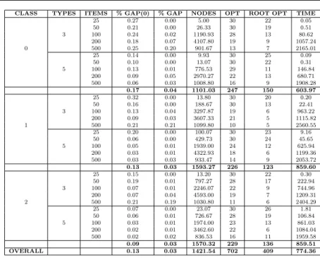
In Table 1 we report the branch-and-price results for classes 0, 1, and 2. In particular, column 1 shows the class number; column 2 the number of bin types; column 3 the number of items, column 4 the percentage gap at the root node, column 5 the residual percentage gap at the end of the branch-and-price; column 6 the number of visited nodes on average, column 7 the number of instances solved to optimality over 900; column 8 the number of instances solved to optimality where the solution found at the root node is also an optimal solution; column 9 the average computing time. Note that the percentage gap at the root node is computed as the difference between the best lower and upper bound at the root node over the best lower bound at the root node; i.e.
U B(0)−LB(0) LB(0)
·100. Note that, sinceLB(0) can be negative, we compute the gap with absolute values. If LB(0) = 0, the gap is set equal to U B(0).
To compute the residual gap at the end of the branch-and-price, we define the best lower bound at the end of the branch-and-priceLBB as follows:
LBB=
U B if the best solution found so far is optimal
LB(0) otherwise.
Then the residual percentage gap is computed as U B−LBB LBB ·100, whereU B is the upper bound corresponding to the best solution found by the branch-and-price.
The results of Table 1 are quite satisfactory: not only we reduce the gap from 0.13% (i.e. the gap calculated at the root node) to 0.03%, but we also solve to optimality 702 instances over 900. The most difficult instances to solve are those with 500 items, and in particular those with 3 bin types. This is justified by the fact that the more the number of items increases, the more the instances are difficult to solve. Moreover, with 3 bin types the choice on the available bins is quite reduced. This makes the problem harder due to the presence of equivalent patterns which increase both the number of variables involved in any column generation iteration and the fragmentation of these variables in the optimal solution of the pricing procedure.
In Table 2 the branch-and-price results for Class 3 are presented. We de-cided to separate Class 3 results from the other classes because these instances are characterized by the presence of both compulsory and non-compulsory items, while the number of items is always 500. Therefore there is not a direct matching with the columns of Table 1. In Table 2 the columns have the fol-lowing meaning: column 1 shows the percentage of compulsory items; column 2 the percentage gap at the root node; column 3 the residual percentage gap after the branch-and-price; column 4 the number of visited nodes on average; column 5 the number of instances solved to optimality over 60; column 6 the number of instances solved to optimality where the solution found at the root node is also an optimal solution; column 7 the average computing time.
The percentage gap at the root node and the residual gap at the end of the branch-and-price are computed as for Table 1. In this case, we solved to optimality 19 instances over 60, i.e. 31% of Class 3 instances. Although the absolute difference of the gap reduction is approximately the same in the two tables (around 0.1%), the residual gap is not as good as in Table 1. This is justified by two issues. First one, the gap at the root node is already high. This is justified by the fact that, for large size instances, 20 seconds of time limit are not enough to computeZSC to optimality. This implies a higher bound at
the root node. The second issue concerns the fact that, as in Class 3 instances both compulsory and non-compulsory items are present, two different sets of constraints are necessary: (2) for compulsory items and (3) for non-compulsory items. This splitting of items with their relative constraints makes the problem harder to solve and justifies the gap growth for Class 3 instances.
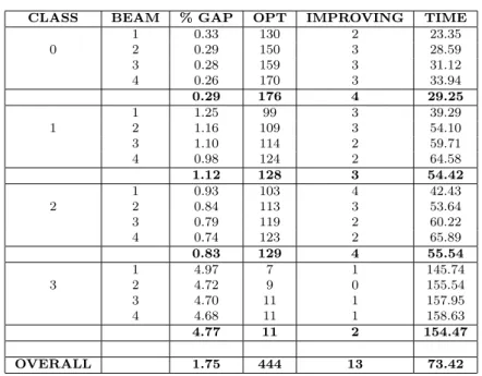
In Table 3 we report our beam search results. In particular, the columns have the following meaning: column 1 shows the class number; column 2 the beam size; column 3 the residual percentage gap after applying the beam search; column 4 the number of instances solved to optimality over 960; col-umn 5 the number of solutions better than those found by the branch-and-price and, finally, column 6 the average computing time. In this table we report all the classes together because we aim to show the overall gap depending on the beam size rather than on the instance attributes. The residual percentage gap is computed in a similar way as for the branch-and-price. Indeed, due to the previous branch-and-price calculation, now we know the optima of many in-stances and we can refer to them when computing the final gap. In particular, given an instance, letU Bbe the best upper bound found by the beam search. Then the residual percentage gap can be computed as
U B−LBB LBB ·100, where LBBvalues are those computed when performing the branch-and-price. If the
branch-and-price could not find an optimal solution, the beam search might find a better solution. However this is quite rare, as it can be seen in column 5 of Table 3. The results show very promising gaps for classes 0, 1, and 2, but not so good for Class 3. This time the high gaps are also justified by the fact that, at the root node, to save time, wedo not compute the ZSC upper
bound which would have improved the accuracy of the method. Of course, increasing the beam size improves the final gap, to the detriment of the
com-CLASS TYPES ITEMS % GAP(0) % GAP NODES OPT ROOT OPT TIME 25 0.27 0.00 5.00 30 22 0.05 50 0.21 0.00 26.33 30 19 0.51 3 100 0.24 0.02 1190.93 28 13 80.62 200 0.18 0.07 4107.80 19 9 1057.24 0 500 0.25 0.20 901.67 13 7 2165.01 25 0.14 0.00 9.93 30 25 0.09 50 0.10 0.00 13.07 30 22 0.31 5 100 0.13 0.01 776.53 29 11 146.84 200 0.09 0.05 2970.27 22 13 680.71 500 0.06 0.03 1008.80 16 9 1908.28 0.17 0.04 1101.03 247 150 603.97 25 0.32 0.00 13.80 30 20 0.20 50 0.16 0.00 188.67 30 13 22.41 3 100 0.13 0.04 3297.87 19 6 963.22 200 0.09 0.03 3607.33 21 5 1115.82 1 500 0.21 0.21 1099.80 10 5 2560.55 25 0.20 0.00 100.07 30 23 9.16 50 0.06 0.00 429.73 30 24 45.65 5 100 0.05 0.01 1939.00 24 12 625.94 200 0.03 0.01 4322.93 18 6 1199.36 500 0.03 0.03 933.47 14 9 2053.72 0.13 0.03 1593.27 226 123 859.60 25 0.15 0.00 13.20 30 22 0.30 50 0.19 0.01 797.27 28 17 222.94 3 100 0.07 0.01 2246.07 22 9 744.96 200 0.07 0.04 4593.00 19 7 1209.31 2 500 0.21 0.19 1030.80 11 6 2404.29 25 0.07 0.00 23.07 30 26 1.81 50 0.06 0.01 726.67 28 19 106.84 5 100 0.03 0.01 1974.00 23 13 861.03 200 0.02 0.01 3462.60 22 6 1084.04 500 0.02 0.02 836.53 16 11 1959.58 0.09 0.03 1570.32 229 136 859.51 OVERALL 0.13 0.03 1421.54 702 409 774.36
Table 1 Branch-and-price results for Classes 0, 1, and 2
PERC. % GAP(0) % GAP NODES OPT ROOT OPT TIME
0 0.11 0.10 1291.33 3 1 2820.44 25 0.32 0.31 1109.00 4 3 2472.01 50 2.11 1.86 1058.50 4 1 2525.91 75 0.47 0.41 1080.17 4 0 2749.93 100 0.21 0.15 1234.33 4 1 2626.93 OVERALL 0.65 0.57 1154.67 19 6 2639.04
Table 2 Branch-and-price results for Class 3
puting time. The relative accuracy of the beam search is highly compensated by the small computing time, which is less than 3 minutes, when the branch-and-price requires, on average, up to 45 minutes. Therefore we can conclude that the proposed beam search is a good compromise between accuracy and computational effort.
7.3 VSBPP comparison
As stated in the Introduction, theV CSBP Pogeneralizes several packing
prob-lems, in particular the VSBPP. Due to its recent introduction, theV CSBP Po
literature is quite limited, while for the VSBPP several heuristic and exact methods are available. In this section we use the proposed branch-and-price and beam search algorithms to address the VSBPP and compare the results
CLASS BEAM % GAP OPT IMPROVING TIME 1 0.33 130 2 23.35 0 2 0.29 150 3 28.59 3 0.28 159 3 31.12 4 0.26 170 3 33.94 0.29 176 4 29.25 1 1.25 99 3 39.29 1 2 1.16 109 3 54.10 3 1.10 114 2 59.71 4 0.98 124 2 64.58 1.12 128 3 54.42 1 0.93 103 4 42.43 2 2 0.84 113 3 53.64 3 0.79 119 2 60.22 4 0.74 123 2 65.89 0.83 129 4 55.54 1 4.97 7 1 145.74 3 2 4.72 9 0 155.54 3 4.70 11 1 157.95 4 4.68 11 1 158.63 4.77 11 2 154.47 OVERALL 1.75 444 13 73.42
Table 3 Beam search results
with those of the state-of-the-art methods specifically designed for the VSBPP, in particularBBHS, the branch and bound presented in Haouari and Serairi
(2011) andV N SHSB, the VNS introduced in Hemmelmayr et al (2012). For
the beam search, we consider the setting with beam size equal to 4. We consider the instance set of Monaci (2002), which was also used by Haouari and Serairi (2011) and by Hemmelmayr et al (2012). Other available VSBPP instances (see, e.g., Alves and Val´erio de Carvalho (2007)) do not seem to be sufficiently challenging, as both the branch-and-price and the beam search are able to solve them to optimality at the root node with a negligible computational time.
Table 4 comparesBBHS with our branch-and-price. The table reports the
number of items in the instances and, for each method, the mean percentage gap between the upper and lower bounds at the root node and the number of instances solved to optimality.BBHS performs better. This is due, as stated
by the authors in their paper, to a series of dominance criteria and lower bounds specifically designed for the VSBPP, which, unfortunately, cannot be extended to theV CSBP Po. For instance, the dominance criteria heavily used
the hypothesis that the number of available bins for each type is infinite, which is not the case for theV CSBP Poand neither for the VCSBPP (Crainic et al,
2011). As expected, since theV CSBP Pois more general, it looses somewhat
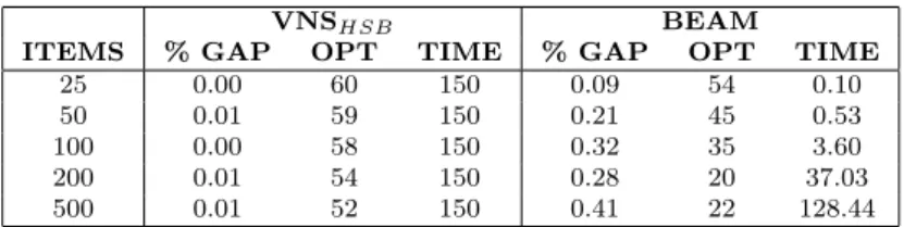
in efficiently proving optimality, but preserves excellent performances in terms of gaps. A similar behaviour can be observed when comparingV N SHSB and
the beam search (Table 5). In this case, the gap remains under 0.5%, within a competitive computational effort (about two minutes in the worst case).
BBHS B&P
ITEMS % GAP OPT % GAP OPT
25 0 60 0 60
50 0.01 59 0 60
100 0.02 59 0.1 57
200 0 60 0.6 41
500 0 60 0.11 29
Table 4 VSBPP results: comparison betweenBBHS and branch-and-price
VNSHSB BEAM
ITEMS % GAP OPT TIME % GAP OPT TIME
25 0.00 60 150 0.09 54 0.10
50 0.01 59 150 0.21 45 0.53
100 0.00 58 150 0.32 35 3.60
200 0.01 54 150 0.28 20 37.03
500 0.01 52 150 0.41 22 128.44
Table 5 VSBPP results: comparison betweenV N SHSB and beam search
8 Conclusion
In this paper we introduced two different methods for solving theV CSBP Po.
The first one is an exact algorithm based on a branch-and-price scheme. From the branch-and-price we then derived a beam search heuristics. We fi-nally presented extensive computational results and showed that most of the V CSBP Po open instances in the literature can be closed.
Future research will be devoted to the introduction of specific cuts for theV CSBP Po and derive from them a branch-and-cut-and-price algorithm.
This is challenging because the conditions for deriving cuts for the VCSBPP and accelerating the column generation available in the literature (Alves and Val´erio de Carvalho, 2007, 2008) do not hold for theV CSBP Po.
Acknowledgements While working on this project, the second author was the NSERC Industrial Research Chair on Logistics Management, ESG UQAM, and Adjunct Professor with the Department of Computer Science and Operations Research, Universit´e de Montr´eal, and the Department of Economics and Business Administration, Molde University College, Norway.
This project has been partially supported by the Ministero dell’Istruzione, Universit`a e Ricerca (MIUR) (Italian Ministry of University and Research), under the 2009 PRIN Project “Methods and Algorithms for the Logistics Optimization”, and the Natural Sciences
and Engineering Council of Canada (NSERC), through its Industrial Research Chair and Discovery Grants programs, and by the partners of the Chair, CN, Rona, Alimentation Couche-Tard and the Ministry of Transportation of Qu´ebec.
References
Alves C, Val´erio de Carvalho JM (2007) Accelerating column generation for variable sized bin-packing problems. European Journal of Operational Re-search 183:1333–1352
Alves C, Val´erio de Carvalho JM (2008) A stabilized branch-and-price-and-cut algorithm for the multiple length branch-and-price-and-cutting stock problem. Computers & Operations Research 35:1315–1328
Baldi MM, Crainic TG, Perboli G, Tadei R (2011) The generalized bin packing problem. Tech. rep., CIRRELT, CIRRELT-2011-39
Baldi MM, Crainic TG, Perboli G, Tadei R (2012) The generalized bin packing problem. Transportation Research Part E 48(6):1205–1220
Belov G, Scheithauer G (2002) A cutting plane algorithm for the one-dimensional cutting stock problem with multiple stock lengths. European Journal of Operational Research 141:274–294
Bettinelli A, Ceselli A, Righini G (2010) A branch-and-price algorithm for the variable size bin packing problem with minimum filling constraint. Annals of Operations Research 179:221–241
Chu C, La R (2001) Variable-sized bin packing: Tight absolute worst-case performance ratios for four approximation algorithms. SIAM Journal on Computing 30:2069–2083
Correia I, Gouveia L, Saldanha-da-Gama F (2008) Solving the variable size bin packing problem with discretized formulations. Computers & Operations Research 35:2103–2113
Crainic TG, Perboli G, Rei W, Tadei R (2011) Efficient lower bounds and heuristics for the variable cost and size bin packing problem. Computers & Operations Research 38:1474–1482
Della Croce F, Ghirardi M, Tadei R (2004) Recovering beam search: Enhancing the beam search approach for combinatorial optimization problems. Journal of Heuristics 10:1381–1231
Desaulniers G, Desrosiers J, Solomon MM (eds) (2005) Column generation. GERAD 25th Anniversary Series, Springer, ISBN 978-0-387-25485-2 Friesen DK, Langston MA (1986) Variable sized bin packing. SIAM Journal
on Computing 15:222–230
Haouari M, Serairi M (2009) Heuristics for the variable sized bin-packing prob-lem. Computers & Operations Research 36:2877–2884
Haouari M, Serairi M (2011) Relaxations and exact solution of the variable sized bin packing problem. Computational Optimization and Applications 48:345–368
Hemmelmayr V, Schmid V, Blum C (2012) Variable neighbourhood search for the variable sized bin packing problem. Computers & Operations Research 39:1097–1108
Hifi H, Michrafy M (2007) Reduction strategies and exact algorithms for the disjunctively constrained knapsack problem. Computers & Operations Re-search 34:2657–2673
ILOG Inc (2009) IBM ILOG CPLEX v12.1 User’s Manual
Kang J, Park S (2003) Algorithms for the variable sized bin packing problem. European Journal of Operational Research 147:365–372
Martello S, Toth P (1990) Knapsack Problems - Algorithms and computer implementations. John Wiley & Sons, Chichester, UK
Monaci M (2002) Algorithms for packing and scheduling problems. PhD thesis, Universit`a di Bologna, Bologna, Italy
Murgolo FD (1987) An efficient approximation scheme for variable-sized bin packing. SIAM - Journal on Computing 16:149–161