A branch-and-cut algorithm for the Time Window
Assignment Vehicle Routing Problem
Kevin Dalmeijer∗ and Remy Spliet Econometric Institute Erasmus School of Economics Erasmus University Rotterdam
October 19, 2016 EI2016-39
Abstract
This paper presents a branch-and-cut algorithm for the Time Window Assignment Vehicle Routing Problem (TWAVRP), the problem of assigning time windows for delivery before demand volume becomes known. A novel set of valid inequalities, the precedence inequalities, is introduced and multiple separation heuristics are presented. In our numerical experiments the branch-and-cut algorithm is 3.8 times faster when separating precedence inequalities. Furthermore, in our experiments, the branch-and-cut algorithm is 193.9 times faster than the best known algorithm in the literature. Finally, using our algorithm, instances of the TWAVRP are solved which are larger than the small scale instances previously presented in the literature. Keywords: Vehicle Routing, Time Window Assignment, Precedence Inequalities. MSC codes: 90B06 (Transportation), 90C11 (Mixed integer programming), 90C57 (Branch-and-cut).
∗E-mail: [email protected]; Phone: +3110 408 9059; Address: PO Box 1738, 3000DR Rotterdam, The Netherlands; Corresponding author
1 Introduction
The Time Window Assignment Vehicle Routing Problem (TWAVRP) is the problem of assigning time windows for delivery to clients in a distribution network when the demand volume of the clients is uncertain, such that the expected transport costs are minimized. First introduced by Spliet and Gabor (2014), the TWAVRP is inspired by distribution networks of retailers.
In a retail network, the clients are retail stores whom place orders on a regular basis. It is common that the time windows for delivery are xed for a long period of time (e.g., a year). This is convenient for the retailers, as it allows them to ensure that enough personnel is available to process the delivery. Furthermore, it simplies inventory control. Demand is uncertain and uctuates per delivery. This results in orders of varying sizes, which become known shortly before the vehicles are dispatched.
To deal with demand uncertainty, the TWAVRP requires demand scenarios and their probability of occurrence to be known in advance. Note that if the number of scenarios is equal to one, the problem reduces to a Vehicle Routing Problem with Time Windows (VRPTW). Hence, the TWAVRP is NP-hard.
An increasing number of companies focus on achieving consistent service with their deliveries (Kovacs et al., 2014). Also in the scientic literature, we see the same trend towards consistency considerations in routing, as can be seen in the recent survey by Kovacs et al. (2014). In this survey, three main pillars of consistency are described: arrival time, person-oriented and delivery consistency, and the TWAVRP is categorized within the rst. Our study adds to the limited amount of research done so far on exact methods for solving routing problems with consistency considerations.
Among the routing problems with consistency considerations, the TWAVRP is in particular closely related to two specic models. Firstly, the TWAVRP is similar to the Consistent Vehicle Routing Problem (ConVRP) introduced in Groër et al. (2009). The ConVRP does not only impose consistent arrival time but also requires the same driver to service the same customer. Another closely related model is the Vehicle Routing Problem with self-imposed time windows, as introduced by Jabali et al. (2015). In their paper, the authors assume demand to be given while travel times are uncertain.
The TWAVRP is a generalization of both the Capacitated Vehicle Routing Problem (CVRP) and the VRPTW, and hence similar solution methods can be used. In a re-cent survey, Baldacci et al. (2012) mention there are three formulations that have been most successful when used to solve the CVRP. Two of them make use of ow variables (Laporte et al. (1985), Baldacci et al. (2004)), while the third is a set partitioning for-mulation (Balinski and Quandt, 1964). For the VRPTW, a set partitioning forfor-mulation in a branch-price-and-cut algorithm is very successful (Desaulniers et al., 2008). To solve the TWAVRP, Spliet and Gabor (2014) also introduce a branch-price-and-cut algorithm based on a set partitioning formulation, which allows for instances with up to 25 clients and three demand scenarios to be solved to optimality within a one hour time limit. Similarly, Spliet and Desaulniers (2015) solve the DTWAVRP, the discrete time window variant of the TWAVRP.
In this paper, we present a new ow formulation for the TWAVRP that is of polynomial size in the number of clients and scenarios. This formulation is based on the MTZ-inequalities in Miller et al. (1960) and the 2-commodity ow formulation in Baldacci et al. (2004). Based on this formulation, we construct a branch-and-cut algorithm that
is faster than the algorithm in Spliet and Gabor (2014). This new algorithm does not only allow for obtaining solutions faster, but also allows for solving larger instances of the TWAVRP, making it applicable to larger networks than previously possible.
One of the factors that contributes to the success of the branch-and-cut algorithm, is the introduction of a novel class of valid inequalities specically designed for the TWAVRP: the precedence inequalities. We identify pairs of routes in dierent scenarios that cannot be selected simultaneously for any feasible time window assignment. Be-cause time windows are not xed in advance, identifying such pairs is a main challenge, which we address. We subsequently create valid inequalities using these pairs, similar to the valid inequalities designed by Ascheuer et al. (2000), which disallow infeasible paths for the Asymmetric Traveling Salesman Problem with Time Windows (ATSPTW). We show that separating precedence inequalities is co-NP-hard and present several separation heuristics to nd violated inequalities.
The remainder of this paper is structured as follows: in Section 2, we present the formu-lation that is used in our and-cut algorithm. In Section 3 we present the branch-and-cut framework. Section 4 is dedicated to the precedence inequalities and heuristics for separating them. Our numerical experiments and their results are presented in Sec-tion 5. In the nal secSec-tion, we write our conclusions and present some direcSec-tions for further research.
2 Problem denition
In this section, we rst formally introduce the TWAVRP. Then, we present a mixed integer linear program to solve the problem.
Consider a set of n clients V0 ={1,2, ..., n}. Furthermore, location 0 represents the
starting depot and location n+ 1 the ending depot. Let V = V0 ∪ {0, n+ 1} represent
the set of all locations. The directed graph Gon vertex setV and with arc set Ais used
to represent our distribution network. Arc set A consists of all arcs leaving the starting
depot, (0, i) for i ∈ V0, all arcs entering the ending depot, (i, n+ 1) for i ∈ V0, and all
arcs between the clients in V0.
For each directed arc(i, j)∈Aa travel costcij and a travel timetij is given. The travel
costs are assumed to be non-negative, cij ≥ 0, and to adhere to the triangle inequality,
cij+cjk ≥cik. We assume the same properties for the travel times. Moreover, we require
all travel times to be strictly positive, the reason for this is highlighted later.
Let wi be the width of the time window that has to be assigned to client i∈V0. We
refer to this time window as the endogenous time window of client i, as opposed to the
exogenous time window of client i which denes the interval in which the endogenous
time window should be chosen. The exogenous time window of each client i∈V0 is xed
and given by the interval[si, ei], withei−si ≥wi. Furthermore, the opening hours of the
starting depot are given by [s0, e0] and the opening hours of the ending depot are given
by[sn+1, en+1].
We assume that we have access to an unlimited number of homogeneous vehicles, each with capacity Q. To model demand uncertainty, consider a nite set of possible demand
scenarios Ω and corresponding probabilities pω such that P
ω∈Ωpω = 1. The demand of
client i∈V0 in scenario ω ∈Ωis given by 0< dω i ≤Q.
time windows within the exogenous time windows and 2), for every demand scenario, a routing of the vehicles adhering to the capacity constraints, and consistent with the assigned endogenous time windows, such that the expected routing cost is minimized.
2.1 Mixed integer linear program
Next, we present a new mixed integer linear programming formulation for the TWAVRP. First we introduce the decision variables. The time window decisions are given by the continuous variables yi for i ∈ V0, which indicate the starting times of the endogenous
time windows. That is, the endogenous time window of client i is given by [yi, yi +wi].
As the endogenous time window has to be within the exogenous time window, we require
yi ∈[si, ei−wi].
The vehicle routes are determined by the binary ow variablesxω
ij for(i, j)∈A, which
are equal to one if a vehicle travels from ito j in scenario ω. The continuous variabletωi
indicates at what time client i∈V0 receives delivery in scenario ω ∈Ω.
For notational convenience, we introduce the arc set A¯. Let A¯ be the set of arcs A
to which the arcs (i,0)and (n+ 1, i)have been added for all i∈V0. To model capacity,
similar to Baldacci et al. (2004), we introduce the ow variables zω
ij for all (i, j) ∈ A¯, ω ∈Ω. Its interpretation depends on the direction the arc is traversed, as given by the
x-variables. If zijω follows this direction (xij = 1), it represents the total vehicle load
when traveling from client i to client j. If it follows the opposite direction (xji = 1), zijω
represents the leftover capacity on the vehicle when traveling from client j to client i. If
the connection between i and j is not used (xij =xji = 0), zijω is zero.
We also introduce the arc sets Aij for all i, j ∈ V. Let Aij be the intersection of A
We provide the following mixed integer linear programming formulation: min X ω∈Ω pω X (i,j)∈A cijxωij (1) s.t. X j∈V0∪{n+1} xωij = 1 ∀i∈V0, ω∈Ω (2) X i∈V0∪{0} xωij = 1 ∀j ∈V0, ω∈Ω (3) zijω +zjiω = X (k,l)∈Aij xωkl Q ∀(i, j)∈A, i < j, ω¯ ∈Ω (4) X j∈V (zjiω −zijω) = 2dωi ∀i∈V0, ω∈Ω (5) X j∈V0 z0ωj = X i∈V0 dωi ∀ω ∈Ω (6) X j∈V0 zωn+1,j = X j∈V0 xω0j ! Q ∀ω ∈Ω (7) X j∈V0 zjω0 = X j∈V0 xω0j ! Q−X i∈V0 dωi ∀ω ∈Ω (8) tωj −tωi ≥tijxωij + (sj −ei)(1−xωij) ∀i∈V 0 , j ∈V0, ω∈Ω (9) s0+t0j ≤tωj ∀j ∈V 0 , ω∈Ω (10) tωi +ti,n+1 ≤en+1 ∀i∈V0, ω∈Ω (11) tωi ≥yi ∀i∈V0, ω∈Ω (12) tωi ≤yi+wi ∀i∈V0, ω∈Ω (13) yi ∈ [si, ei−wi] ∀i∈V0 (14) xωij ∈ B ∀(i, j)∈A, ω ∈Ω (15) zijω ≥0 ∀(i, j)∈A, ω¯ ∈Ω. (16)
The objective (1) is to minimize the expected traveling costs over all scenarios. Con-straints (2) and (3) are the ow conservation conCon-straints. ConCon-straints (15) make sure all ows are integral.
Vehicle capacity is modeled by Constraints (4)-(8) and (16), which are based on the 2-commodity ow formulation in Baldacci et al. (2004). Constraints (4) relate opposing arcs: when either (i, j) or(j, i) is used, the corresponding z-variables sum to the vehicle
capacity.
Constraints (5) can be seen as ow conservation constraints for thez-variables: before
visiting the client, the load is dω
i units more than afterwards. After visiting, the empty
space isdωi units more than before. Hence, the total dierence in both ows is equal to2dωi.
The total vehicle load, capacity and excess capacity in the system are constrained by (6)-(8). Constraints (6) set the total vehicle load equal to the total demand of all clients, and Constraints (7) set the total capacity equal to the number of used vehicles multiplied by the vehicle capacity. The total excess capacity of all vehicles leaving the starting depot is set by Constraints (8). Finally, we enforce vehicle capacity to be respected by constraining
all empty space on the vehicles to be non-negative, as is done in Constraints (16). For more details on these constraints, see Baldacci et al. (2004).
Constraints (9)-(14) deal with the time windows. Constraints (9) are the MTZ-inequalities that model the time-of-service (Miller et al., 1960). If a vehicle travels from client i to client j in scenario ω ∈ Ω, then xω
ij = 1 and hence tωj −tωi ≥ tij, i.e., the
time-of-service increases with at least the travel time from i to j. If no vehicle travels
from i toj in scenario ω, then xω
ij = 0and the constraint reads tωj −tωi ≥sj−ei, which
always holds as tω
j ≥ sj and tωi ≤ ei. Note that the MTZ-inequalities eliminate cycles,
because we have assumed that tij >0for all (i, j)∈A.
Constraints (10) guarantee that vehicles can only leave the starting depot after it opens and Constraints (11) ensure that vehicles arrive at the ending depot before it closes. Constraints (12) and (13) enforce that each client is served within its endogenous time window, while Constraints (14) make sure these endogenous time windows are within the exogenous time windows.
2.2 Remarks
In the above formulation, we model capacity using constraints that are based on the 2-commodity ow formulation in Baldacci et al. (2004). The MTZ inequalities are used to model time-of-service. Other formulations for capacity and time-of-service have been considered as well, including several adaptations of models for the CVRP (Baldacci et al., 2004) and the ATSPTW (Ascheuer et al., 2001).
Preliminary testing with all our combinations of capacity constraints and time-of-service constraints in a branch-and-cut algorithm showed that the best performance is achieved by the combination of the 2-commodity ow formulation to model capacity and the MTZ-inequalities to model time-of-service. This may seem surprising, as in general the MTZ-inequalities typically do not contribute to strong bounds in the LP relaxation. For our instances, however, we have seen that this is compensated for by the relatively strong formulation for capacity.
The MTZ-inequalities require no additional variables and onlyn(n+1)|Ω|constraints.
This allows for a branch-and-cut strategy in which we process the nodes of the search tree faster than in all other alternatives we considered. Using the 2-commodity ow formulation to model capacity yields a good trade-o between the number of variables and constraints, and the strength of the formulation.
3 Branch-and-cut algorithm
In this section, we present our branch-and-cut algorithm. First, we present valid inequal-ities from the literature, which we use to strengthen the LP-bound of (1)-(16). Next, we introduce our branching strategy. In Section 4 we separately introduce the novel precedence inequalities.
3.1 2-cycle elimination
The current mixed integer linear program ensures that no integer feasible solution contains cycles. Explicit cycle elimination, however, may still strengthen the LP-bound.
As there are only a quadratic number of 2-cycles in a given graph, we can eliminate all 2-cycles with a relatively small number of constraints. We do so by adding all of the
following inequalities to the formulation:
xωij +xωji ≤1 ∀i∈V0, j ∈V0, ω ∈Ω. (17)
3.2 Rounded capacity inequalities
The capacity inequalities are well-known valid inequalities for the VRPTW, and thus may be applied directly to the TWAVRP per scenario. Let λω
S be the minimum number
of vehicles required to satisfy the demand of all clients in S ⊆ V0 in scenario ω. The
capacity inequalities are given by X
(i,j)∈A|i∈S,j∈V\S
xωij ≥λωS ∀S ⊆V0,|S| ≥2, ω ∈Ω. (18)
That is, we require for each subset S⊆V0 that the total number of vehicles leaving S is
sucient to satisfy all demand in S.
Calculating λωS requires solving a bin-packing problem, which is NP-hard in general.
Hence, as is commonly done, we only consider the weakened inequalities in which λω S
is replaced by the bin-packing lower bound d P
i∈Sdωi
/Qe. These valid inequalities
are known as the rounded capacity inequalities. Simply adding all rounded capacity inequalities is not ecient, but when used in a branch-and-cut algorithm, they can be very eective (Baldacci et al., 2012).
We add the following |Ω| inequalities to the formulation:
X i∈V0 xωi,n+1 ≥ P i∈V0dωi Q ∀ω ∈Ω. (19)
The other rounded capacity inequalities are separated and added in a cutting plane fashion. We use the separation algorithm from Lysgaard (2003). Details on this algorithm can be found in Lysgaard et al. (2004).
3.3 Branching strategy
In the formulation in Section 2.1, we require each xω
ij to be binary. However, we show
that it is sucient to require that all xωij ∈[0,1], thatxωij is binary for all arcs connected
to one of the depots, and furthermore that xω
ij +xωji is binary for all i, j ∈V
0(i6=j). We dene the following integrality conditions:
xω0j ∈B ∀j ∈V0, ω∈Ω, (20)
xωi,n+1 ∈B ∀i∈V0, ω ∈Ω, (21)
xωij +xωji ∈B ∀i < j, i∈V0, j ∈V0, ω ∈Ω, (22)
xωij ∈[0,1]∀(i, j)∈A, ω ∈Ω. (23)
Proposition 1. All integer feasible solutions to (1)-(14), (16), (17), (19), and (20)-(23) satisfy
xωij ∈B ∀(i, j)∈A, ω∈Ω. (15)
Proposition 1 suggests that for any i, j ∈ V0 instead of branching on whether a single
directed arc is used, we may also branch on whether a connection between i and j
(regardless of direction) is used. This decision can be made per connection, as xωij ∈ B
and xω
ji∈B together implyxωij+xωji ∈B,xωij ∈[0,1]and xωji∈[0,1]. That is, Proposition
1 is still applicable if for some connections we branch on both xω
ij and xωji and for the
other connections we branch on xωij +xωji.
Branching on xij means that we partition the feasible region in two parts. In the
rst part it is assumed thatj is visited directly afteri by the same vehicle. In the other
part we assume j is not visited directly after i. Knowing whether j is visited directly
after i has important implications for the time-of-service variables tωi and tωj. The value
(sj−ei)in the MTZ-inequalities is essentially a big-M, hence fractional values of the ow
variables cause the time constraints to be very weak or inactive. Whenxωij = 1, however,
we have tωj ≥ tωi +tij. Especially when tij is big, this inequality has a big eect on the
time-of-service variables.
If the value of tij is close to zero, this argument no longer holds, whether xij = 1 or xji = 1is not that important for the time-of-service variables. For the capacity constraints
it is important to know whether i and j are visited by the same vehicle, but it is less
important to know in which order this happens. Hence, it makes sense to branch on
xij +xji to split the feasible region in two parts: one part in which j is visited directly
after i, or the other way around, and one part in which there is no direct connection
between i and j.
To take these eects into account, we introduce the parameter ρ ∈ [0,1]. Then, for
the fraction ρ of all arcs with the shortest travel time, we branch on the connections.
For the other arcs, we branch on xω
ij and xωji separately. Note that ρ = 0 corresponds
to always branching on individual arcs. If ρ = 1, we always branch on connections. By
varying ρ, a good compromise can be found between the number of variables and the
strength of the LP relaxation.
4 Precedence inequalities
In this section, we present a novel set of valid inequalities, the precedence inequalities, in which each inequality involves multiple scenarios. First, we make some important observations.
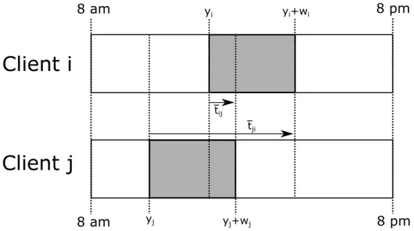
If we want to visit rst i and later j, both within their respective time windows, the
time between the two visits is bounded. Let¯tij be the maximum time between these visits,
for all i, j ∈V0. That is, we dene ¯tij = (yj+wj)−yi and similarly tji¯ = (yi+wi)−yj,
as illustrated in Figure 1. It follows thatt¯ij + ¯tji =wi+wj.
Now consider a solution to the TWAVRP for which in scenario ω there is a route
visiting rst i, and later j. Furthermore, assume there is a dierent scenario ω0 with a
route visiting rst j, and later i. It follows that the time taken to get from i to j in one
scenario, plus the time taken to get from j to i in another scenario, can be at most the
sum of the widths of the time windows, wi +wj.
We formalize this in Observation 2. LetAp be the set of arcs used by pathpinGand
letPij be the set of all elementary paths in G starting at i∈V and ending at j ∈V.
Observation 2. For given vertices i, j ∈V0 (i6= j), for any integer feasible solution to
8 am
8 pm
tij tji yj yi yj+wj yi+wi8 am
8 pm
Client i
Client j
Figure 1: Example time window assignment and maximum allowed driving times. used in scenario ω0 ∈Ω the following holds:
X (k,l)∈Ap tkl+ X (k,l)∈Aq tkl ≤wi+wj. (24)
To construct valid inequalities based on Observation 2, we make use of Theorem (4.5) in Ascheuer et al. (2000), which we restate for the TWAVRP as the following lemma. Lemma 3. For any integer feasible TWAVRP solution, a set of clients S ⊆ V0 and two
vertices i, j ∈V0\S (i6=j), a single vehicle visits i rst, then all clients in S and then j
consecutively in scenario ω ∈Ω if and only if:
X l∈S xωil+X k∈S X l∈S xωkl+X k∈S xωkj +xωij =|S|+ 1. (25)
Lemma 3 gives us a criterion for testing whether there is a path visiting client i, then
visiting a subset of other clients, and then visiting client j. Combining this lemma with
Observation 2 allows us to formulate the precedence inequalities.
Let us denote by (S : T) the set of arcs in A which start in S and end in T, for S and T vertices or sets of vertices. For notational convenience we introduce the sets
S(i, j) = {S | S ⊆ V0\{i, j}} for all i, j ∈ V0. That is, S(i, j) is the set of all possible
subsets of clients not containing clients i and j. When traveling from i to j, visiting
exclusively clients from S, only the arcs in (i:S)∪(S :S)∪(S :j)∪(i:j) are relevant.
Therefore, we introduce F(i, S, j) ={F | F ⊆(i:S)∪(S :S)∪(S :j)∪(i: j)}, which
for given i, j ∈V0 and S ∈ S(i, j) is the set of all possible subsets of these arcs.
Furthermore, let δij(S, F) be the shortest possible travel time from client i ∈ V0 to
client j ∈ V0, visiting all clients in S ∈ S(i, j) in between, using only arcs from set
F ∈ F(i, S, j). If no such path existsδij(S, F) =∞. We then arrive at the main theorem
for the precedence inequalities:
Theorem 4. Precedence inequalities: For given scenarios ω, ω0 ∈ Ω (ω 6= ω0), given
scenario ω, and vertex set S0 ∈ S(j, i) corresponding to clients visited in scenarioω0, and
given arc setsF ∈ F(i, S, j)andF0 ∈ F(j, S0, i)such thatδij(S, F)+δji(S0, F0)> wi+wj,
the following are valid inequalities: X
(k,l)∈F
xωkl+ X
(k,l)∈F0
xωkl0 ≤ |S|+|S0|+ 1. (26)
Proof. This is a direct application of Observation 2. Lemma 3 shows that Observation 2 is contradicted if and only if P
(k,l)∈F x ω kl+ P (k,l)∈F0xω 0 kl =|S|+|S 0|+ 2. By integrality of the x-variables, the theorem follows.
It is possible to generalize this result by redening δij(S, F)to be the minimum travel
time to visit clienti, all clients inS and then clientj using only arcs of F, but only using
paths that can be feasible when considering the exogenous time windows. We choose not to present this generalization, as we consider an application in which the exogenous time windows are in general very wide. The proposed generalization is then unlikely to add much value, while making it more complex to identify violated inequalities.
Clearly, the number of possible precedence inequalities is exponential in the number of clients. Hence, it is not ecient to add all precedence inequalities to the formulation directly. Instead, we separate the precedence inequalities in a cutting plane fashion. Note that exact separation of the precedence inequalities is dicult, as nding violated precedence inequalities is co-NP-hard, which is proven in Appendix B. For this reason, we separate subsets of the precedence inequalities exactly, and we present heuristics for more general precedence inequalities.
Before we consider these subsets, we state the following two lemmas, which will be useful when deriving our separation algorithms. We provide a lower bound on the ow in F for violated inequalities and we show that for every violated inequality F is cyclic
orF contains an elementary (i, j)-path visiting all vertices in S.
Lemma 5. Let i, j ∈ V0, S ∈ S(i, j), S0 ∈ S(j, i), F ∈ F(i, S, j) and F0 ∈ F(j, S0, i)
correspond to a violated precedence inequality, for a feasible solution to the LP relaxation of the formulation (1)-(16), (17) and (19). Then both
X (k,l)∈F xωkl >|S| (27) and X (k,l)∈F0 xωkl0 >|S0|. (28)
Proof. By denition ofF(i, S, j)all directed arcs inF point to vertex j, or to a vertex in S. Thus, by the ow conservation constraints it follows that the total ow inF is bounded
by|S|+1. Hence, we haveP (k,l)∈F x ω kl≤ |S|+1and similarly P (k,l)∈F0xω 0 kl ≤ |S 0|+1. From Theorem 4 it follows that for a violated precedence inequalityP
(k,l)∈Fx ω kl+ P (k,l)∈F0xω 0 kl >
|S|+|S0|+ 1. Combining these facts proves the lemma.
Lemma 6. Let i, j ∈ V0, S ∈ S(i, j), S0 ∈ S(j, i), F ∈ F(i, S, j) and F0 ∈ F(j, S0, i)
correspond to a violated precedence inequality, for a feasible solution to the LP relaxation of the formulation (1)-(16), (17) and (19). Then F contains a cycle or F contains an
elementary (i, j)-path through all vertices of S. Also F0 contains a cycle or F0 contains
Proof. We prove this statement for F, as for F0 the proof is analogous. If F contains a
cycle, the lemma holds. Next, we assumeF is acyclic. Moreover, we assume that F does
not contain an elementary path from i toj through all vertices of S, and we show that
this leads to a contradiction.
BecauseF is acyclic, the vertices ofS can be relabeledv1, v2, . . . , v|S|such that ifl < k then (vk, vl)∈/ F (see Kahn (1962)). By assumption, there is no elementary path from i
through allv1, v2, . . . , v|S| toj. Hence, there exists an integerg ∈ {1,2, . . . ,|S| −1}such that there is no arc from vg to vg+1.
Let U1 = {i, v1, v2, . . . , vg−1} and let U2 = {vg+2, vg+3, . . . , v|S|, j}. By construction, we have that X (k,l)∈F xωkl = X (k,l)∈ U1:(U1∪vg∪vg+1∪U2) T F xωkl + X (k,l)∈ (vg∪vg+1∪U2):U2 T F xωkl ≤ |U1|+|U2|=|S|. (29)
This follows because the total outow of the vertices inU1 is bounded by|U1| due to the
ow conservation constraints. Similarly, the total inow of the vertices in U2 is bounded
by|U2|. Hence, it follows that the total ow captured byF is bounded by|U1|+|U2|=|S|.
This contradicts Lemma 6, which states thatP
(k,l)∈F xωkl>|S|. Thus, our assumption
that F does not contain an elementary path from i through S to j is false. Hence, we
have proven that F contains a cycle, or contains an elementary (i, j)-path visiting all
clients in S.
4.1 Path precedence inequalities
The rst subset of precedence inequalities we consider, is the subset for which F and F0
both form a single elementary path, which we refer to as the path precedence inequalities. We make use of the following proposition:
Proposition 7. For any integer feasible solution to the TWAVRP: X (k,l)∈Ap tkl+ X (k,l)∈Aq tkl > wi+wj =⇒ X (k,l)∈Ap xωkl+ X (k,l)∈Aq xωkl0 ≤ |Ap|+|Aq| −1 ∀(i, j)∈A, p∈Pij, q ∈Pji, ω∈Ω, ω0 ∈Ω. (30)
Proof. This is a direct application of Theorem 4 with F = Ap and F0 = Aq. Note that δij(S, F) =
P
(k,l)∈Aptkl, as following the path p is the only way to visit all vertices in S using only vertices in F. Analogously, δji(S0, F0) =
P
(k,l)∈Aqtkl. Finally, note that
|S|=|Ap| −1and |S0|=|Aq| −1, and hence|S|+|S0|+ 1 =|Ap|+|Aq| −1.
Proposition 7 denes valid inequalities for paths only, instead of for arbitrary sets of vertices and arcs. Next, we show some properties of the path precedence inequalities. These properties are then used to prove that for a given solution to the LP relaxation, all violated path precedence inequalities can be found in polynomial time.
Lemma 8. All violated path precedence inequalities adhere to the following two inequali-ties:
X
(k,l)∈Ap
X
(k,l)∈Aq
xωkl0 >|Aq| −1. (32)
Proof. This is a direct application of Lemma 5 with F =Ap and F0 =Aq.
Lemma 9. Let p and q correspond to a violated path precedence inequality. Path p in
graph G contains at most one arc (k, l) for which xw kl ≤
1
2. Path q contains at most one
arc (k0, l0) for which xω0 k0l0 ≤ 12.
Proof. Suppose p has m ≥2 arcs for which xω kl ≤ 1 2. This implies P (k,l)∈Apx ω kl ≤ |Ap| − 1
2m≤ |Ap| −1. Hence (31) is not satised. It follows thatphas at most one arc for which
xω
kl ≤ 12. The proof for path q is analogous.
Proposition 10. All violated path precedence inequalities can be found in polynomial time.
Proof. To nd all violated path precedence inequalities, we generate an exhaustive list of candidate paths fromi toj which meet the necessary condition given by Lemma 9. If we
do the same for all candidate paths from j toi, we can check for all combinations of the
candidates whether (30) is violated.
To generate a list of candidates, we rst use Lemma 9, which states that for scenario
ω ∈ Ω a candidate uses at most one arc for which xωkl ≤ 1
2. Starting at i, the path thus
rst uses a (possibly zero) number of arcs for which xω kl>
1
2, followed by zero or one arcs
for which xω kl ≤
1
2. After that, we visit another (possibly zero) number of arcs for which
xωkl > 12 before we reach j.
By the ow conservation constraints, the total outow and the total inow of a vertex are both equal to one. Hence, at each vertex there can be at most one incoming arc and one outgoing arc for which xωkl > 12. This implies there is at most one elementary path
leaving i for which all arcs have an x value larger than 1
2. Analogously there is at most
one elementary path entering j for which all x values are larger than 12. Finding these
two elementary paths takes O(n2) time, as the paths contain O(n) vertices, and, for a
single vertex, determining which arc has value larger than 1
2 takes O(n) time.
All candidate paths from itoj can thus be constructed by starting in i, following the
arcs with x values larger than 12 up to a certain point after which an arc with x value
less or equal to 1
2 is taken to arrive at the path of arcs with x values larger than 1 2 that
arrives at j, which is followed until we reach j. That is, without loss of generality we
sequentially visit the vertices i=v1, v2, . . . , vf, wg, wg−1, . . . , w1 =j for integers f and g
between 1and n.
For givenf andg, the total ow of the candidate path is given byPf−1
i=1 xvivi+1+xvfwg+
Pg−1
i=1 xwi+1wi, and the total travel time is given by
Pf−1
i=1 tvivi+1+tvfwg+
Pg−1
i=1 twi+1wi. By
precalculating the summations for allf andg inO(n2)time, this part only takes constant
time.
For each scenario, there are O(n2) combinations of f and g. We thus nd O(|Ω|n2)
candidates from i to j. Then, we check for all combinations of candidates from i to j
and candidates from j toiif the condition in Proposition 7 is satised. Per combination,
this takes constant time, as we only sum the predetermined values of total ow and total travel time. There are O((|Ω|n2)2) such combinations. As we repeat the procedure for
4.2 Tournament precedence inequalities
In the previous section, we have introduced the path precedence inequalities, which are precedence inequalities based on elementary paths. In this section we present a broader subset of the precedence inequalities, in which both(S, F)and(S0, F0)represent a directed
acyclic graph. Furthermore, we show that to satisfy all these valid inequalities it is sucient to restrict ourselves to those directed acyclic graphs F and F0 obtained by
taking the transitive closures of an elementary path. The transitive closure of a set of arcs F ⊆A in graph G, is dened as follows:
trcl(F) :={(k, l)∈A:l can be reached from k using only arcs in F}. (33)
These inequalities are similar to the tournament constraints of Ascheuer et al. (2000), hence we call this class the tournament precedence inequalities. In Ascheuer et al. (2000), the tournament inequalities are introduced for the ATSPTW, which are obtained by bounding the total ow on the transitive closure of a simple path which violates (ex-ogenous) time window constraints or cannot be extended without violating time window constraints. Next we present the tournament precedence inequalities, discuss how to sep-arate them, and show that if all tournament precedence inequalities are satised then so are all precedence inequalities based on directed acyclic graphs.
Proposition 11. For any integer feasible solution to the TWAVRP: X (k,l)∈Ap tkl+ X (k,l)∈Aq tkl > wi+wj =⇒ X (k,l)∈trcl(Ap) xωkl+ X (k,l)∈trcl(Aq) xωkl0 ≤ |Ap|+|Aq| −1 ∀(i, j)∈A, p∈Pij, q ∈Pji, ω∈Ω, ω0 ∈Ω. (34)
Proof. This is a direct application of Theorem 4 with F = trcl(Ap) and F0 = trcl(Aq).
Observe that taking the transitive closure of an elementary path yields a directed acyclic graph, which contains only a single path visiting all vertices. In particular, δij(S, F) = δij(S,trcl(Ap)) =δij(S, Ap) =P(k,l)∈Aptkl. Similarly, δji(S, F) =
P
(k,l)∈Aqtkl. Note that
|S|=|Ap| −1and |S0|=|Aq| −1, and hence|S|+|S0|+ 1 =|Ap|+|Aq| −1.
Corollary 12. If a path precedence inequality is violated, then its corresponding tourna-ment precedence inequality (by taking transitive closures) is violated as well.
Proof. Follows directly from Proposition 11, the non-negativity of the x variables and F ⊆trcl(F)for all F ⊆A.
As a result, we can nd violated tournament precedence inequalities by separating path precedence inequalities. However, not all violated tournament precedence inequalities can be found in this way. Hence, to separate all tournament precedence inequalities, we next present another algorithm.
First, per scenario, we make a list of all elementary paths in G, not involving the
depot vertices. By denition, each tournament precedence inequality is characterized by two elementary paths and two scenarios. Hence, after we generate the lists, we can separate the tournament precedence inequalities by combining elementary paths from the lists, and checking the condition given in Proposition 11 for each pair.
To construct the list per scenario we use a procedure similar to that described in Ascheuer et al. (2001) to detect violated tournament constraints for the ATSPTW. We
enumerate all paths but backtrack as soon asP
(k,l)∈trcl(Ap)x ω
kl ≤ |Ap| −1. It is suggested
in Ascheuer et al. (2001) that only a polynomial number of paths is generated this way, which would imply that our separation routine, involving multiple scenarios, also requires only a polynomial number of iterations.
We have mentioned that, for separating tournament precedence inequalities, restrict-ing to transitive closures of elementary paths still allows us to capture all precedence inequalities based on directed acyclic graphs. We state this formally in the following lemma.
Lemma 13. Let i, j ∈ V0, S ∈ S(i, j), S0 ∈ S(j, i), F ∈ F(i, S, j) and F0 ∈ F(j, S0, i)
correspond to a precedence inequality, for a feasible solution to the LP relaxation of the formulation (1)-(16), (17) and (19). Furthermore, assume F and F0 are acyclic. If all
tournament precedence inequalities are satised, then this precedence inequality is also satised.
Proof. AsF is assumed to be acyclic, by Lemma 6 it contains an elementary pathp∈ Pij
through all vertices of S. By denition of the transitive closure, it follows that F ⊆
trcl(Ap). Analogously we have F0 ⊆trcl(Aq) for someq ∈ Pji visiting all vertices of S0.
We haveP (k,l)∈Fx ω kl+ P (k,l)∈F0xω 0 kl ≤ P (k,l)∈trcl(Ap)x ω kl+ P (k,l)∈trcl(Aq)x ω0 kl ≤ |S|+|S 0|+
1, as all tournament precedence inequalities are assumed to be satised. It follows that
if all tournament precedence inequalities are satised, each precedence inequality based on directed acyclic graphs is satised as well.
4.3 Additional strategies
We have discussed two subsets of the precedence inequalities with corresponding separa-tion strategies. There are, however, some addisepara-tional strategies that can be utilized.
Note that both the separation algorithm for the path precedence inequalities and the separation algorithm for the tournament precedence inequalities rst generate a list of viable candidates i, j ∈ V, S ∈ S(i, j) and F ∈ F(i, S, j) per scenario, after which
all combinations of candidates are checked to nd violated inequalities. An additional strategy is to opportunistically alter these candidates when combining them to create stronger inequalities.
Recall that one way to do this, is by separating path precedence inequalities and taking transitive closures, resulting in tournament precedence inequalities (Corollary 12). Another strategy is to complete F by adding arcs. That is, let F∗ be the maximum
cardinality element ofF(i, S, j). By denition, F∗ = (i:S)∪(S :S)∪(S :j). Note that
F∗ is not acyclic, and hence in general δij(S, F∗)6=δij(S, F). Furthermore, δij(S, F∗) is
hard to calculate.
Therefore, we introduce an easy to calculate lower bound onδij(S, F∗). Note that any
violated precedence inequality found while using this lower bound is valid for the actual value of δij(S, F∗)as well. It is well known that the weights of a minimum spanning tree
can be used as a lower bound on the length of the shortest elementary path visiting all vertices. It thus follows that:
δij(S, F∗)≥min
k∈S {tik}+MST(S) + mink∈S {tkj}, (35)
in which MST(S) represents the weight of the minimum weight spanning tree of an
undirected complete graph with vertex set S and edge weight min{tkl, tlk} for each edge
We consider the following strategies. First, separate either path precedence inequal-ities or tournament precedence inequalinequal-ities. The path precedence inequalinequal-ities may be converted to tournament precedence inequalities. Each resulting tournament precedence inequality corresponds to sets i, j ∈ V0, S ∈ S(i, j), F ∈ F(i, S, j), S0 ∈ S(j, i) and
F ∈ F(j, S, i). Now try whether a violated precedence inequality can be obtained by
replacingF byF∗ and/orF0 byF0∗, using the lower bounds on travel time given by (35).
If so, use these stronger valid inequalities.
5 Numerical experiments
Next, we present the results of our numerical experiments to test the eectiveness of our new formulation, the precedence inequalities and the branching strategy. Furthermore, we present experiments in which our algorithm is compared to the branch-price-and-cut algorithm of Spliet and Gabor (2014).
All experiments are run on an Intel i7 3.5GHz computer with 16GB of RAM. To allow for a fair comparison between algorithms, we restrict all experiments to a single thread on a single core. As a basis for our implementation, we use the commercial solver CPLEX version 12.5, with default settings. We disable all CPLEX's built in valid inequalities, so we can more accurately test the eect of the valid inequalities discussed in this paper.
Our own valid inequalities will be generated in a callback, which is called each time the LP relaxation has been solved, or re-solved after adding valid inequalities. In this callback we separate rounded capacity inequalities and precedence inequalities, and only afterwards the LP is resolved. We use the built-in `traditional branch-and-cut' in combi-nation with our own branching strategy as discussed in Section 3.
For our branch-and-cut algorithm we use the 64 bit version of CPLEX, which allows for the full 16GB of memory to be used. The algorithm of Spliet and Gabor (2014) requires less memory, and hence we use the 32 bit version of CPLEX, which gives a slightly better performance.
We use a one hour time limit per instance in all experiments. From preliminary tests we have found that almost every instance is unsolvable within the time limit without separating rounded capacity inequalities, so we separate those in all experiments.
5.1 Test-instances
First, we introduce the dierent sets of test-instances which we use for our numerical experiments.
5.1.1 Small instances
We use forty instances introduced by Spliet and Gabor (2014). These instances are randomly generated instances, inspired by a Dutch retail chain. The set contains ten instances of 10, 15, 20 and 25 clients respectively. The clients are uniformly distributed over a square with sides of length ve. Both the starting depot and the ending depot are located in the center of the square. The travel cost and the travel time in hours between two points in the square is equal to the Euclidean distance.
Each instance includes three demand scenarios, each with equal probability of oc-currence. The average demand is about 1/6 vehicle load. The exogenous time windows
are rather wide: on average the exogenous time window of the client has width 10.8, compared to an endogenous time window width of 2.
5.1.2 Large instances
To be able to test our branch-and-cut algorithm on larger instances as well, we have generated fty additional instances in the same way that the small instances have been generated. That is, we created ten instances of 30, 35, 40, 45 and 50 clients respectively. All instances are available online.
5.2 Branch-and-cut experiments
Next, we compare the branching strategies and the separation algorithms for the prece-dence inequalities, using the forty small instances. We consider six dierent strategies to separate precedence inequalities, which have been detailed in Section 4.3:
N Do not separate precedence inequalities. P Separate path precedence inequalities. P2T 1) Separate path precedence inequalities.
2) Turn them into tournament precedence inequalities. P2C 1) Separate path precedence inequalities.
2) Turn them into tournament precedence inequalities.
3) CompleteF and/orF0 by adding additional arcs and add corresponding
vio-lated precedence inequalities if they are found. T Separate tournament precedence inequalities. T2C 1) Separate tournament precedence inequalities.
2) CompleteF and/orF0 by adding additional arcs and add corresponding
vio-lated precedence inequalities if they are found.
For the branching strategy, we conduct experiments for ρ ∈ {0,0.1, ...,1}. Recall that
this corresponds to a strategy in which we branch on connections for the the fraction ρ
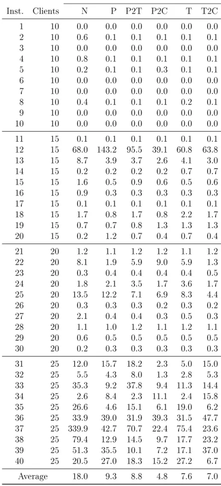
of arcs with the shortest travel time. For the other connections, we branch on arcs. In Table 1 we have reported solution times for all combinations of separation and branching strategies. These numbers are aggregated values obtained by computing the average over the forty instances.
We see that strategies P2T and P2C are the best performers for most choices of ρ.
Setting ρ 6= 0 yields a positive eect for all separation strategies, although the exact
value of ρ does not seem to be that important. In the remainder of the experiments,
we will use the combination of ρ = 0.6 and P2C, as this combination yields the lowest
average solution time on our test set. If we compare the solution time of the combination of ρ = 0.6 and P2C to the solution time of the combination of N and ρ = 0, we see
that introducing the precedence inequalities and the branching strategy together yields a factor 6.6 improvement in solution time.
In Table 2, results of using the dierent separation strategies are presented forρ= 0.6.
The rows respectively present the average solution time in seconds, the average number of visited nodes of the search trees, the average number of precedence inequalities and
Seconds Separation strategy ρ N P P2T P2C T T2C 0.0 31.8 27.2 20.2 18.6 33.9 36.2 0.1 13.7 10.4 7.1 7.6 8.2 8.7 0.2 13.5 5.7 9.3 5.4 9.3 7.3 0.3 13.2 6.8 6.5 5.5 7.5 8.8 0.4 12.0 10.1 6.3 6.9 8.4 8.0 0.5 11.1 7.2 5.7 6.5 8.7 7.8 0.6 18.0 9.3 8.8 4.8 7.6 7.0 0.7 10.4 8.5 7.9 6.8 10.2 7.8 0.8 21.4 9.8 9.9 7.1 9.9 10.6 0.9 12.3 9.5 8.7 5.3 8.6 6.0 1.0 22.5 11.9 9.6 6.2 9.0 5.4
Table 1: Average solution times for various strategies.
rounded capacity inequalities added, and the percentages of the total solution time used for the separation of the precedence inequalities and for the rounded capacity inequalities. The last row displays for how many out of the forty instances the used separation strategy yielded the shortest computation time. If multiple strategies have the same solution time (rounded to milliseconds), they are all counted as best strategies.
N P P2T P2C T T2C
Seconds 18.0 9.3 8.8 4.8 7.6 7.0
Nodes 2,481 1,406 1,144 537 848 696
Precedence inequalities 0 117 107 66 97 101
Rounded capacity inequalities 575 426 413 341 405 390 % of time sep. prec. 0.0% 5.4% 6.2% 4.4% 8.0% 8.0% % of time sep. cap. 2.7% 3.3% 3.0% 2.7% 3.0% 2.6% Best strategy 6/40 9/40 9/40 14/40 7/40 14/40 Table 2: Average branch-and-cut statistics for various separation strategies(ρ= 0.6).
If we look at the total solution time, it becomes clear that all strategies yield an im-provement over strategy N. Based on the tested instances, strategy P2C yields the lowest computation time; a factor 3.8 better than strategy N.
Looking at the number of nodes in the search trees, we see that all strategies allow the number of nodes to be greatly reduced compared to strategy N. We see that, on average, using T2C allows for the largest number of violated precedence inequalities to be found per node in the search tree. Still, strategy P2C is more eective. This observation cannot be explained by the increase in separation time alone; the average time spend per instance on separating precedence inequalities is 0.2 seconds for P2C, and 0.6 seconds for T2C.
There are two other eects that may explain the dierence between P2C and T2C. First, as more precedence inequalities are found, larger LP relaxations have to be solved, which takes more time. Second, as more precedence inequalities can be found, it can
happen that the LP relaxation is resolved more often. It seems that this additional work does not add much value over P2C.
Table 2 shows that P2C is the best strategy for 14 of the test-instances. For T2C, this number is the same. Looking at the disaggregated data (Table 5 in Appendix C) we see that for the instances with 20 clients, T2C is the best strategy 5 out of 10 times, while P2C is never the best strategy. For the instances with 25 clients, however, P2C is the best strategy 5 out of 10 times, while T2C is the best only once.
Surprisingly, after processing only the root node, there is almost no dierence in lower bounds between strategy N and the other strategies. For 35 instances the lower bounds are exactly the same. For the other instances, dierences between lower bounds of at most 0.04% are observed. The power of the precedence inequalities really shows further down in the search tree. This could be explained by the nature of the precedence inequalities: they disallow certain combinations of paths. If a solution is very fractional, not many paths can be detected, and hence the precedence inequalities are of little use. Deeper in the tree, where more variables are xed, they become more eective.
5.3 Comparison with branch-price-and-cut
Next, we compare the performance of our branch-and-cut algorithm, using strategy P2C and ρ = 0.6, to the performance of the branch-price-and-cut algorithm in Spliet and
Gabor (2014).
To this end, we run their implementation on the same computer as on which our algorithm is run. The computation times are thus directly comparable. The results we present are based on their branch-price-and-cut algorithm with 2-cycle elimination and adding rounded capacity cuts, which is the solution method in Spliet and Gabor (2014) yielding the best average time performance on the test set.
The results per instance can be found in Table 3. Per instance, data is provided on ve dierent categories, both for the price-and-cut algorithm (BP&C) and the branch-and-cut algorithm (B&C). The columns labeled `Seconds' indicate the times in seconds for solving the instance to optimality, the maximum time allowed being one hour. The columns `Nodes' state the number of nodes of the search tree that have been explored during that time. When the algorithm terminates, the percentual deviation from the optimum is given in the column `Optimality gap'. A value of zero indicates the problem was solved to optimality. The column `Root gap' shows a similar value, indicating the optimality gap after processing only the root node. The optimality gap and the root gap are calculated ex-post, using the actual optimal value. Finally, the column `Value' gives the optimal objective value for that instance.
Seconds Nodes Optimality gap Root gap Value Inst. Clients BP&C B&C BP&C B&C BP&C B&C BP&C B&C B&C
1 10 0.7 0.0 1 1 0 0 0 0 17.65 2 10 121.9 0.1 483 18 0 0 0.17 0.28 15.56 3 10 3.7 0.0 1 1 0 0 0 0 17.42 4 10 28.5 0.1 193 6 0 0 0.14 0.14 18.51 5 10 2.3 0.3 2 42 0 0 0 0.34 16.07 6 10 1.5 0.0 2 1 0 0 0 0 18.00 7 10 4.9 0.0 4 1 0 0 0 0 17.02 8 10 3.5 0.1 29 21 0 0 0.65 0.96 23.89 9 10 3.0 0.0 7 1 0 0 0 0 20.31 10 10 5.9 0.0 5 1 0 0 0 0 16.31 11 15 87.4 0.1 22 1 0 0 0 0 17.78 12 15 3,600.0 39.1 889 14,037 0.15 0 0.67 2.36 27.10 13 15 3,600.0 2.6 684 587 0.59 0 1.10 1.78 29.37 14 15 58.0 0.2 45 1 0 0 0 0.03 23.18 15 15 29.4 0.6 36 11 0 0 0 0.17 24.15 16 15 92.4 0.3 98 1 0 0 0.10 0.17 21.03 17 15 22.9 0.1 15 1 0 0 0 0 22.04 18 15 105.3 0.8 98 124 0 0 0.20 0.47 22.30 19 15 133.3 1.3 133 210 0 0 0.56 0.97 26.52 20 15 41.6 0.4 28 11 0 0 0 0 22.11 21 20 3,600.0 1.2 864 48 0.02 0 0.57 1.11 28.08 22 20 152.3 9.0 62 658 0 0 0.03 0.19 29.80 23 20 99.6 0.4 40 1 0 0 0 0.12 30.30 24 20 112.2 1.7 27 58 0 0 0.03 0.86 24.16 25 20 3,600.0 6.9 712 389 0.08 0 0.61 1.09 29.84 26 20 65.4 0.2 16 1 0 0 0 0 29.72 27 20 85.5 0.3 24 1 0 0 0 0 26.48 28 20 106.5 1.1 36 11 0 0 0 0.08 26.14 29 20 65.5 0.5 17 1 0 0 0 0.05 26.61 30 20 45.1 0.3 4 1 0 0 0 0 26.36 31 25 610.9 2.3 121 20 0 0 0.13 0.57 31.43 32 25 840.0 1.3 164 4 0 0 0.07 0 30.71 33 25 3,600.0 9.4 413 395 0.33 0 0.45 1.03 33.71 34 25 193.2 11.1 36 391 0 0 0 0.33 33.34 35 25 640.0 6.1 119 201 0 0 0 0.85 29.05 36 25 3,600.0 39.3 1,662 1,733 0.13 0 0.43 1.49 30.50 37 25 3,600.0 22.4 278 1,472 0.29 0 0.29 0.43 28.68 38 25 3,600.0 9.7 1,259 337 0.12 0 0.30 0.59 35.69 39 25 3,600.0 7.2 2,294 219 0 0 0.50 0.94 32.55 40 25 1,093.2 15.2 521 471 0 0 0.30 0.62 32.14 Average 931.4 4.8 286.1 537.2 0.04 0 0.18 0.45 25.29
What immediately stands out is the enormous decrease in computation time of our new algorithm with respect to the previous algorithm. The instances that can be solved to optimality by the branch-price-and-cut algorithm, can be solved to optimality by the branch-and-cut algorithm 89.6 times faster on average. In total, 9 instances cannot be solved to optimality by the branch-price-and-cut algorithm after a total of 9 hours of computation time. With the branch-and-cut algorithm, all these instances can be solved to optimality in 137.9 seconds. Hence, this is a speedup of at least a factor 234.9.
The new algorithm is faster for all tested instances by at least a factor 7.6 and even up to a factor 2997 for instance 21. If we consider the time necessary to attempt to solve all instances combined, the total time decreases from 37,255.3 seconds in total to 192.1 seconds; a speedup factor of 193.9. We point out that this dierence is not the result of using rounded capacity cuts, as both the branch-and-cut algorithm and the branch-price-and-cut algorithm use these valid inequalities.
It can be seen that an advantage of the branch-price-and-cut algorithm is the stronger LP bound it provides, as for almost all instances the root gap is smaller than the gap given by the branch-and-cut algorithm. However, this strength is less apparent in the remainder of the search tree, as on average the branch-and-cut algorithm processes only twice the number of nodes in the branch-price-and-cut algorithm. There are some extreme instances, however, where processing a lot of nodes is necessary, e.g., instances 12 and 36. Here, we observe that the branch-and-cut algorithm is able to process a large number of nodes in little time (14000+ in less than 40 seconds for instance 12). The branch-price-and-cut algorithm generates stronger bounds, but cannot process enough nodes in the given time to solve the problem.
5.4 Performance on larger instances
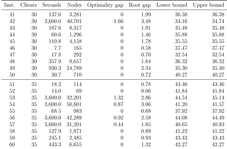
As our branch-and-cut algorithm is able to solve all 40 test-instances used in Spliet and Gabor (2014), we also test our algorithm on larger instances, as introduced in Section 5.1. Recall that these instances are generated in a similar way as the rst forty instances. The only dierence is that the number of clients is larger: between 30 and 50.
In Table 4 we report results for the instances with 30 and 35 clients. This table is structured in the same way as Table 3. The column `Value' is replaced by the columns `Lower bound' and `Upper bound', as not all instances can be solved to optimality. The reported root gaps are no longer ex post, but based on the best known upper bound.
It can be seen that all but one of the instances with 30 clients can be solved to optimality within one hour of computation time, and for the remaining instance we nd a solution with an optimality gap of 1.66%.
The instances with 35 clients are more dicult: 6 out of the 10 instances can be solved to optimality within one hour. The remaining instances have an optimality gap of less than 1.32%.
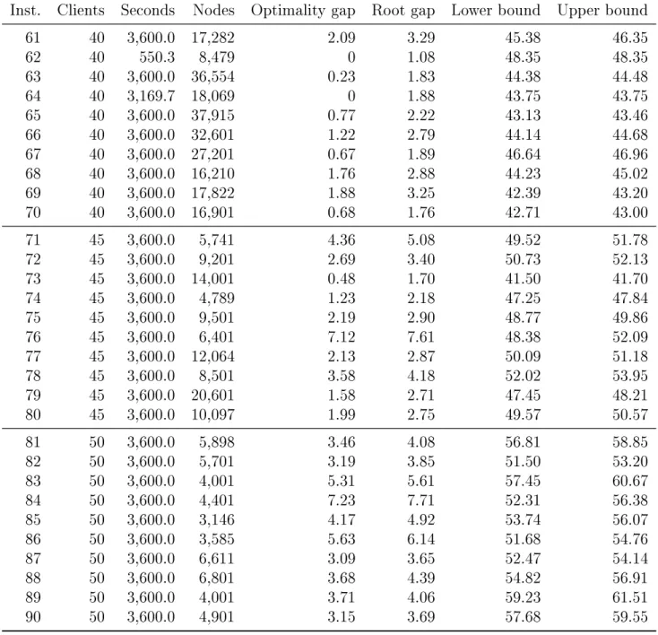
The instances with 40, 45 and 50 customers cannot be solved consistently by our branch-and-cut algorithm, which proves optimality of the found solution for only two of these instances in one hour of computation time. In Table 6 in Appendix C, we report the results for these instances, including best found lower and upper bounds. The instances with 40 clients have optimality gaps below 2.09%. The instances with 45 clients have optimality gaps between 0.48% and 7.12%. The instances with 50 clients have optimality gaps between 3.09% and 7.23%.
Inst. Clients Seconds Nodes Optimality gap Root gap Lower bound Upper bound 41 30 137.0 3,281 0 1.99 36.38 36.38 42 30 3,600.0 40,701 1.66 3.48 34.16 34.74 43 30 187.6 8,317 0 1.91 35.48 35.48 44 30 60.6 1,296 0 1.46 35.88 35.88 45 30 110.8 4,158 0 1.78 35.55 35.55 46 30 7.7 165 0 0.58 37.47 37.47 47 30 17.8 292 0 0.70 32.54 32.54 48 30 357.9 9,657 0 1.84 36.32 36.32 49 30 930.3 24,789 0 2.34 35.30 35.30 50 30 30.7 710 0 0.72 40.27 40.27 51 35 18.2 114 0 0.78 43.46 43.46 52 35 14.0 69 0 0.06 41.84 41.84 53 35 3,600.0 32,201 1.32 2.86 44.54 45.14 54 35 3,600.0 50,601 0.87 3.06 41.20 41.57 55 35 68.5 983 0 0.68 37.92 37.92 56 35 3,600.0 42,289 0.92 2.58 44.08 44.49 57 35 3,600.0 31,201 0.44 1.85 40.65 40.83 58 35 127.9 1,871 0 0.89 41.22 41.22 59 35 245.1 2,485 0 0.93 43.43 43.43 60 35 443.3 6,655 0 1.32 42.27 42.27
6 Conclusion
In this paper we present a compact formulation for the TWAVRP based on the 2-commodity ow formulation introduced by Baldacci et al. (2004) and the MTZ-inequalities introduced by Miller et al. (1960). We use this formulation in a branch-and-cut algorithm in which rounded capacity cuts are separated in each node of the search tree.
To further improve the performance of our algorithm, we introduce a branching rule and a novel class of valid inequalities: the precedence inequalities. These TWAVRP specic inequalities are hard to separate in general. Therefore, we introduce exact sepa-ration algorithms for two subsets, the path precedence inequalities and the tournament precedence inequalities. Furthermore, we extend these algorithms to separation heuristics for general precedence inequalities. Using the branching rule and separating precedence inequalities makes our algorithm 6.6 times faster.
The new algorithm is superior to the best known algorithm in the literature, the algorithm of Spliet and Gabor (2014), for all tested instances. Overall, an average speedup factor of 193.9 is achieved.
Finally, we test our algorithm on larger instances. Of the instances with 30 clients, 9 out of 10 instances could be solved to optimality within the one hour time limit. For the instances with 35 clients, we found the optimal solution for 6 out of 10 instances. The instances that could not be solved to optimality all have an optimality gap of less than 1.66%. Instances with 40 clients and more, however, could not be solved to optimality consistently.
In this paper, we compare our results to the branch-price-and-cut algorithm of Spliet and Gabor (2014). Even without the use of precedence inequalities, our algorithm shows a substantial speedup over the branch-price-and-cut algorithm. It it still interesting, though, to investigate the eect of incorporating the precedence inequalities in a branch-price-and-cut algorithm. Similarly, it is interesting to see how the precedence inequalities would perform on the DTWAVRP.
Another interesting topic of further research concerns algorithms for separating prece-dence inequalities. In the future, TWAVRP algorithms would benet from new algorithms for separating the remaining class of precedence inequalities, corresponding to directed cyclic graphs.
References
Norbert Ascheuer, Matteo Fischetti, and Martin Grötschel. A Polyhedral Study of the Asymmetric Traveling Salesman Problem with Rime Qindows. Networks, 36(2):6979, 2000.
Norbert Ascheuer, Matteo Fischetti, and Martin Grötschel. Solving the Asymmetric Travelling Salesman Problem with time windows by branch-and-cut. Mathematical Programming, 90(3):475506, 2001.
Roberto Baldacci, Eleni Hadjiconstantinou, and Aristide Mingozzi. An Exact Algorithm for the Capacitated Vehicle Routing Problem Based on a Two-Commodity Network Flow Formulation. Operations Research, 52(5):723738, 2004.
Roberto Baldacci, Aristide Mingozzi, and Roberto Roberti. Recent exact algorithms for solving the vehicle routing problem under capacity and time window constraints. European Journal of Operational Research, 218(1):16, 2012.
Michel L Balinski and Richard E Quandt. On an Integer Program for a Delivery Problem. Operations Research, 12(2):300304, 1964.
Guy Desaulniers, François Lessard, and Ahmed Hadjar. Tabu Search, Partial Elemen-tarity, and Generalized k-path Inequalities for the Vehicle Routing Problem with Time Windows. Transportation Science, 42(3):387404, 2008.
Chris Groër, Bruce Golden, and Edward Wasil. The Consistent Vehicle Routing Problem. Manufacturing & service operations management, 11(4):630643, 2009.
Ola Jabali, Roel Leus, Tom Van Woensel, and Ton De Kok. Self-imposed time windows in vehicle routing problems. OR Spectrum, 37(2):331352, 2015.
Arthur B Kahn. Topological Sorting of Large Networks. Communications of the ACM, 5(11):558562, 1962.
Attila A Kovacs, Bruce L Golden, Richard F Hartl, and Sophie N Parragh. Vehicle Routing Problems in Which Consistency Considerations are Important: A Survey. Networks, 64(3):192213, 2014.
Gilbert Laporte, Yves Nobert, and Martin Desrochers. Optimal Routing under Capacity and Distance Restrictions. Operations research, 33(5):10501073, 1985.
Jens Lysgaard. CVRPSEP: A package of separation routines for the Capacitated Vehicle Routing Problem. Working paper, Aarhus School of Business, 2003.
Jens Lysgaard, Adam N Letchford, and Richard W Eglese. A new branch-and-cut al-gorithm for the capacitated vehicle routing problem. Mathematical Programming, 100 (2):423445, 2004.
Clair E Miller, Albert W Tucker, and Richard A Zemlin. Integer Programming Formu-lation of Traveling Salesman Problems. Journal of the ACM (JACM), 7(4):326329, 1960.
Christos H Papadimitriou. The Euclidean travelling salesman problem is NP-complete. Theoretical Computer Science, 4(3):237244, 1977.
Remy Spliet and Guy Desaulniers. The discrete time window assignment vehicle routing problem. European Journal of Operational Research, 244(2):379391, 2015.
Remy Spliet and Adriana F Gabor. The Time Window Assignment Vehicle Routing Problem. Transportation Science, 49(4):721731, 2014.
A Proof Proposition 1
Proposition 1. All integer feasible solutions to (1)-(14), (16), (17), (19), and (20)-(23) satisfy
xωij ∈B ∀(i, j)∈A, ω∈Ω. (15)
Proof. Constraints (20) and (21) state that xω
0j, xωj,n+1 ∈ B for all j ∈ V0. Next, we
will prove that if xωij = 1 with i ∈ V0 ∪ {0} and j ∈ V0, then there exists a unique k ∈V0∪ {n+ 1},k 6=i such thatxω
jk = 1.
Suppose that xω
ij = 1 for some i∈V0∪ {0} and j ∈V0. Due to the ow conservation
constraints xωlj = 0 for all l 6= i and furthermore there exists a vertex k ∈ V0 ∪ {n+ 1}
such that xω
jk > 0. If k = n+ 1, then by integrality of the ows going into the depot,
we have xω
jk = 1 and by the ow conservation constraints we have xωjl = 0 for all l 6=k.
Finally, supposek 6=n+ 1. Note thatk 6=iasxjk >0whilexji = 0becausexij+xji = 1.
Constraints (22) and (23) state thatxω
jk+xωkj = 1 and sincexωlj = 0 for alll 6=i, it follows
that xω
jk = 1. Using again the ow conservation constraints, xjl= 0 for all l6=k.
We know that all ows out of the depot are equal to one. We have just proven that any vertex in V0 with a single inow of 1 also has a single outow of 1. It follows that
all ows between the depots are of size 1.
What remains to be proven is that all clients are contained in the integral ows be-tween the depots. Because of the ow conservation constraints (2)-(3), the only other possibility is that there exists a cycle, given by edges(1,2),(2,3), ...,(k−1, k),(k,1)such
that for each arc (i, j) in this cycle we have xωij +xωji = 1. Using the ow conservation
constraints (2)-(3), we have that all arcs adjacent to this cycle have zero ow. Con-straints (4) and (16) together state that if xij +xji = 0, then zij = zji = 0. Hence, if a
cycle exists, (5) contains the following constraints:
zk,ω1−z1ω,k+z2ω,1−z1ω,2 = 2dω1 z1ω,2−z2ω,1+z3ω,2−z2ω,3 = 2dω2
...
zkω−1,k−zk,kω −1+z1ω,k −zωk,1 = 2dωk
Summing these constraints gives 0 = 2Pk
i=1dωi >0, which is a contradiction. Hence, all
clients are contained in the integer ows between the depots. It follows that allx-variables
B Separating precedence inequalities is co-NP-hard
We prove that separating precedence inequalities is co-NP-hard. First, we present a brief outline of the proof.We construct a specic instance of the TWAVRP and a corresponding optimal solution to the LP relaxation of (1)-(16), (17) and (19). This optimal solution to the LP relax-ation is an instance of the separrelax-ation problem of nding violated precedence inequalities. We will refer to this instance as instance I. Next, we characterize this instance of the
separation problem as a decision problem. Finally, we show that separating precedence inequalities is co-NP-hard. We show this by a polynomial time reduction from Euclidean TSP.
TWAVRP instance
Considern≥4clients, travel timestij adhering to the triangle inequality, and endogenous
time window widthswi. Lettmax be the maximum of the given travel times, and letwmax
be the maximum of the given endogenous time window widths.
We setsi = 0andei = 2tmax+wmaxfor all locationsi∈V and we dene two scenarios
Ω ={1,2}, both with probability 0.5 of occurring. In both scenarios, we set the demand
of every client equal to 1. The vehicle capacity Q is set equal to n. We set all travel
costs equal to zero, such that any feasible solution to the LP relaxation is also an optimal solution.
Solution to the LP relaxation
Next, we describe an optimal solution to the LP relaxation. We start with setting the
x-variables. For scenario 1, set x11i = x1ij = x1in = n−12 for all i = 2,3, . . . , n−1 and
j = 2,3, . . . , n−1 (i6= j) and set x1
01 =x1n,n+1 = 1. All other x-variables for scenario 1
are set to zero.
For scenario 2, we setx201 =x2n,n+1 = 1− 1
n−1. Furthermore, we setx 2
0i =x2i,n+1 = 1for
all i= 2,3, . . . n−1. Moreover, we set x2
0n =x21,n+1 = 1 and x2n1 = 1
n−1. The remaining
ow variables are set to zero.
As an example, Figures 2 and 3 present the ows given by thex-variables whenn = 4.
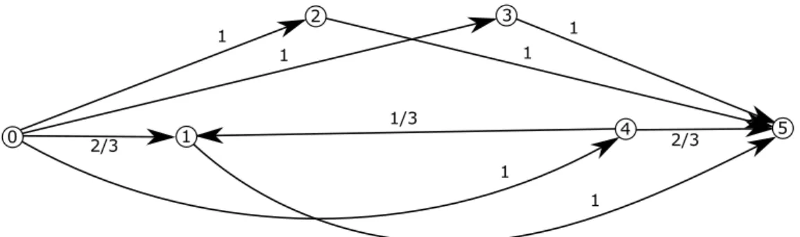
1/2 1/2 1/2 1/2 1/2 1/2 1 1 0 1 2 3 4 5
Figure 2: Flows given by the x-variables in scenario 1 when n= 4.
Next, we also present an assignment for the z-variables. For scenario 1 we set z1 01 =
zn1+1,n = n. Furthermore, we set z11i = zni1 = nn−−12 and z1i1 = zin1 = n−12 for all i = 2,3, . . . , n−1. Finally, we set z1
ij = n
n−2 for all i= 2,3, . . . , n−1 and j = 2,3, . . . , n−1
(i6=j). All other z-variables are set to zero.
For scenario 2 we set z012 = nn−−21, z102 = n−2, z02n = nn−1, z2n0 = n− n n−1, z 2 1n = 1, z2 n1 = 1 n−1, z 2 n+1,1 =n, zn2+1,n = n(n−2) n−1 and nally z 2 0i = 1, z2i0 =n−1and zn2+1,i =n for
alli= 2,3, . . . , n−1. All remainingz-variables are set to zero.
Finally, set yi =tmax for all i∈V0 and tωi =tmax for all i∈V
1 1 1 1 1 1 1/3 2/3 2/3 0 2 1 4 3 5
Figure 3: Flows given by the x-variables in scenario 2 when n= 4.
It is straightforward to check that the described variables give a feasible solution to the LP relaxation of (1)-(16), (17) and (19). As all costs are equal to zero, this solution is also optimal. By denition, our optimal solution to the LP relaxation is an instance of the separation problem. In the remainder, we refer to this instance of the separation problem as instance I.
Characterization as a decision problem
Next, we characterize instance I of the separation problem as a decision problem. First,
we prove the following lemma.
Lemma 14. If instance I contains a violated precedence inequality, then the only violated
precedence inequality is given by (using the notation of Theorem 4) i = 1, j = n, S =
{2,3, . . . , n−1}, F = (1 :S)∪(S :S)∪(S :n), S0 =∅ and F0 ={(n,1)}.
Proof. By denition, F0 cannot contain arcs involving the depot vertices. Therefore,
considering the assigned values of the x-variables in scenario 2, we have that the arc
(n,1) is the only arc with non-zero ow that may be in F0. Hence, P
(k,l)∈F0x2kl = 0 if
(n,1) ∈/ F0 or 0 < P
(k,l)∈F0x2kl = n−11 < 1 if (n,1) ∈ F0. By Lemma 5 we have that
P
(k,l)∈F0x2kl > |S0| ≥ 0. Thus, (n,1) is contained in F0. Using that
P
(k,l)∈F0x2kl < 1
and P
(k,l)∈F0x2kl > |S0| it follows that |S0| = 0 and hence S0 = ∅. As S0 = ∅ and
(n,1)∈ F0, it follows that i = 1, j =n and F0 = {(n,1)}. It remains to be shown that
S ={2,3, . . . , n−1} and F = (1 :S)∪(S:S)∪(S :n).
Suppose by contradiction that S ∈ S(1, n) is such that |S| ≤ n−3. In this case, the
largest setF ∈ F(1, S, n)is given byF = (1 :S)∪(S :S)∪(S :n). Therefore, the number
of arcs inF is bounded by|1 :S|+|S :S|+|S :n|=|S|+|S|(|S| −1) +|S|=|S|(|S|+ 1).
For instanceI, all these arcs have ow equal to n−12. It follows thatP
(k,l)∈F x1kl ≤ |S|(|S|+
1)n−12 for allS ∈ S(1, n)andF ∈ F(1, S, n). Recall thatP
(k,l)∈F0x2kl= n−11 and |S0|= 0.
Using |S|+ 1 ≤ n−2 we derive P
(k,l)∈F x1kl+
P
(k,l)∈F0x2kl ≤ |S|(|S|+ 1)n−12 + n−11 ≤
|S|+|S0|+ 1for all |S| ≤n−3. By Theorem 4, the corresponding precedence inequality
is not violated, which is a contradiction. It follows that |S| = n −2, which implies
S ={2,3, . . . , n−1}.
Finally, we show that F = (1 :S)∪(S :S)∪(S :n) by contradiction. Suppose that
F 6= (1 :S)∪(S : S)∪(S : n). Recall that S ={2,3, . . . , n−1} and thus |S| =n−2.
Therefore,|F| ≤ |S|(|S|+ 1)−1 = (n−2)(n−1)−1. Hence,P (k,l)∈Fx 1 kl+ P (k,l)∈Fx 2 kl ≤ ((n−2)(n−1)−1)n−12 + n−11 = n −1− 1 n−2 + 1 n−1 ≤ n−1 = |S|+|S 0|+ 1, which is a contradiction of the precedence inequality being violated. It follows that F = (1 :