Biometric Identification using Electroencephalography

(1)

Biometric Identification using Electroencephalography

ABSTRACT

In this paper, investigate the use of brain activity for person identification. A biometric system is a technological system that uses information about a person. Research on brain signals show that each individual has a unique brain wave pattern. Electroencephalography signals generated by mental tasks are acquired to extract the distinctive brain signature of an individual. Electroencephalography signals during four biometric tasks, namely relax, math, read and spell was acquired from 50 subjects. Features are derived from power spectral density. Classification is performed using Feed forward neural network and Recurrent neural network. The performance of the neural model was evaluated in terms of training, performance and classification accuracies. The results confirmed that the proposed scheme has potential in classifying the EEG signals. RNN is considerably better with an average accuracy of 95% for the spell task and 92% for the read tasks in comparison with a feed forward neural network. The results validate the feasibility of using brain signatures for biometrics study.

Keywords

Biometric Authentication, EEG Signal Process, Power Spectral Density, Feed Forward Neural Network and Recurrent Neural Network.

1. INTRODUCTION

In recent years, a new application of brain waves has emerged, namely the use of EEG recordings as a biometric. Biometric authentication is a method that can be used to uniquely identify or authenticate a person based on individual physiological and behavioral characteristic. The characteristic is measurable and unique. Physiological biometrics that are currently used are fingerprints, DNA, iris scans and hand palm scans for authentication purposes. Behavioral biometrics is gait, voice recognition, which relates to analyzing the behavior of a person. A biometric system provides two functions, namely verification and identification. In verification, the system validates a person’s identity by comparing the captured biometric data with his/her own biometric template stored system database. While verification system recognizes an individual by searching the templates of all the users in the database for a match. Therefore, thesystem conducts a one-to-many comparison to establish an individual’s identity [1]. The fundamental barriers in biometrics can be grouped into four main categories such as (i) accuracy (ii) scale (iii) security and (iv) privacy.

Electroencephalography (EEG) is generally referred an a act of recording an electrical activity along the scalp. It measures the voltage fluctuations which results in an ionic current flow between the neurons of the brain. EEG measures mostly the currents that flow during synaptic excitations of the dendrites of many pyramidal neurons in the cerebral cortex. The cortex

is a dominant part of the central nervous system. The highest influence of EEG comes from electric activity of cerebral cortex due to its surface positions [1-4]. Electroencephalography (EEG) is becoming increasingly popular as a new modality in biometric authentication which has several advantages as it is confidential, difficult to mimic and almost impossible to steal. This paper presents a new method for person identification using brain EEG signal processing. Six feature extraction algorithm are compared to design a biometric authentication system using neural network.

2. LITERATURE REVIEW

Some researches on EEG based biometrics have been studied [1]-[4]. EEG can be used as a biometric modality since the EEG signals can be acquired non-invasively from six to eight electrodes. Mental tasks for biometric verifications have been proposed by Paranjape et al. and Ravi and palaniappan with minimal electrodes on a limited dataset [5] [6]. A study by Paranjape et al. reported that EEG biometric potential signals were able to discriminate 40 different subjects with autoregressive features derivated from 8 channels. The maximum classification accuracy rate is 82% [6]. Riera et al. collected data from 51 subjects and 36 intruders. The EEG was recorded from 2 channels while subjects were sitting with eyes closed for 1 minute. They obtained a true acceptance rate of 96.6% and false acceptance rate of 3.4% [7]. Hema et al. recorded EEG signals from 3 electrodes for 6 subjects with Power Spectral Density features using Welch algorithm to extract the features and a feed forward neural network with three layers were used to classify. Three mental tasks, namely relax, read and spell were able to achieve an average authentication rate of 97% [8].

Poulos et al. collected single channel EEG signals from 75 subjects in one session and obtained a classiﬁcation rate of 91%, thus corroborating the evidence that the EEG signals carry genetically septic information that are suitable for person identification. Poulus et al. and Poulus et al. collected single channel of EEG signals for 4 subjects resting with eyes closed. Features extracted from the autoregressive model parameters or the FFT based spectral analysis with a learning vector quantized network were classified. They obtained maximum accuracy of around 80% and 100% [9] [10]. Ravi and Palaniappan used a total of 61 channels and recorded VEP EEG signals for 20 subjects. The extracted beta waves were processed using principal component analysis to extract the features and two classifiers were used, namely fuzzy ARTMAP and k-nearest neighbor.The maximum average classification rate is 95% [11]. Jiang Feng Hu recorded EEG signal identiﬁcation using 6 channels for 10 subjects. The extracted beta waves were processed using the Welch algorithm. The maximum accuracy ranges obtained was 75% - 80% for authentication and 75% -78.3% for identification

Hema C.R

Faculty Of Engineering, Karpagam University,

Coimbatore, India,

Elakkiya. A

Research Scholar Karpagam University

Coimbatore

Paulraj MP

(2)

[12]. Palaniappan and Ravi, further investigated features based on the spectral power of the signal together with a fuzzy neural network for the classification. More recently Gaussian mixture models and maximum a posterior model adoption has

been proposed in S’ebastien et.al [13].

The literature available on biometrics using EEG shows that the biometric studies have been made using EEG signals collected using 2 to 61 channels. However, to design a real time biometric system, number of channels to be used and tasks assigned to the subjects to evoke the EEG signals have to be optimized to simplify the acquisition process. Hence, in this research, the use of a single channel acquisition process for various tasks suitable for biometrics are proposed and studied.

3. DATA ACQUISITION

EEG signal is recorded using a single channel AD Instrument biosignal amplifier. The sampling frequency is fixed at 200Hz. Three gold plated cup shaped electrodes are placed at F4, O2, Fp1 locations based on the International 10-20 Electrode Placement System (Fig1). EEG signals were collected from 50 subjects (15females and 35 males). All of them were either University students or staff members. The age group of the subjects was between 15 to 45 years. The subjects were seated comfortably in a noise free room and requested to perform the tasks mentally without any overt movements. The subjects were requested to perform four mental tasks, namely Relax, Read, Spell and Math tasks. Each task was repeated for ten trials and each trial lasts for 10 seconds with breaks of 10 minutes between trials. The data were collected in two sessions on different days. 40 data samples were collected per subjects, total 2000 data samples are acquired from all 50 subjects.

The protocol for the four tasks performed by the individuals are as detailed below.

Task 1- Relax: The subject is requested to sit in a relaxed manner. The subject should be still without moving the entire body for 10 seconds. This task is used as a baseline measure of the EEG. Task2- Read: The subject is shown a typed card with tongue twister sentences and they are requested to read the sentence mentally without vocalizing.

Task3- Spell: The subject is shown a typed card with his/her name and is requested to spell his name mentally without vocalization and overt movements.

Fig.1. Electrode placement location for data acquisition

Task4- Math activity: The subject is given five non trivial multiplication problems, such as 789 multiplied by 885, and is asked to solve them for 10 seconds without moving the entire body.

4. PRE-PROCESSING AND FEATURE

EXTRACTION

EEG signals are very noisy and they can be easily affected by electrical activity of the eyes or muscles. During acquisition a notch filter is applied to remove the 50Hz noise due to electrical power source. To improve the quality of the signal, preprocessing of the raw data is performed. The raw EEG signals are acquired and segmented into four frequency bands, namely delta (0.5-3 Hz), theta (3-7 Hz), alpha (7 – 12 Hz) and beta (12- 40 Hz). Among the four, alpha and beta are seen in the conscious state of a human. Hence, these are consider the frequency bands alpha and beta from the original frequency bands. The EEG signals are band pass filtered using twelve frequency bands from the alpha and beta rhythms of 7 Hz to 42 Hz with a bandwidth of 3 Hz. Chebychev filter is used to segment the signals in 3Hz band frequency in the range of 7Hz to 42Hz . The 12 band pass signals are ((7-10) Hz, (10-13) Hz,(13-16) Hz,(16-19) Hz, (19-21) Hz, (21-24) Hz, (24-27) Hz, (27-30) Hz, (30-33) Hz,(33-36) Hz, (36-39) Hz, (39-42) Hz. This segmentation is used to remove the lower range noise frequencies from 0.1 Hz to 6 Hz arising due to EOG signals and EMG signals above 43 Hz. 12 signal segments are obtained from the pre-processed EEG signals. In this study, feature patterns are extracted from the EEG signals using following six PSD algorithms.

Power spectral density of the segmented signals is estimated and used as features. Power spectral density describes how the energy of a signal or a time series is distributed with frequency. The power spectral density of six algorithms are compared in this study.The power spectral density of six different algorithms are covariance, modified covariance, music, burg, Welch and yule-walker.

4.1. Covariance Method

In the Power Spectral Density using covariance method, all the data points are needed to compute the prediction error power estimates. No zeroing of the data is necessary. The AR parameter estimates the solution of the equations which can be written as:

Based upon this

c 1,0 … … c p, 0 +

c 1,1 … … c 1, p … … … c p, 1 … c p, p

a 1 … … a (p) =

0 …

0 (1)

𝑐 𝑗, 𝑘 =

_𝑁−𝑃1 𝑁−1

𝑥

∗

𝑛=𝑃

(𝑛 − 𝑗𝑥(𝑛

-k) (2)

PSD estimation is formed as:

p

cov

=

σ

2

1+ p_k=1a k .e−j2π fk₂

3

The power spectral density using the covariance method gives the distribution of the power per unit frequency and the pre order of AR model [13] [14] [15] .

(3)

Fig.2. Plot for power spectral density using covariance method for subject 1 for spell task

4.2. Burg Method

Burg technique performs the minimization of the forward and backward prediction errors and estimates the reflection coefficient. From the estimations of the AR parameters, PSD estimation is expressed as given . This process dimensionally reduces the signal data to 12 features [13] [14] [15] .

𝑝 𝐵𝑢𝑟𝑔 𝑓

= 𝑒 2𝑝

1 + 𝑝𝑖=1𝑎 𝑝 𝑖 𝑒−2𝜋𝑖𝑓

2 (4)

The major advantage of the Burg Method is that in high frequency resolution, AR model is always stable and computationally very efficient.

Frequency (Hz)

Fig.3. Plot for power spectral density using burg method for the subject for spell task

4.3. Modified Covariance Method

The modified covariance methods estimate the AR parameters by minimizing the average of the estimated forward and backward prediction error power. The modified covariance for estimating the spectral content fitting an autoregressive (AR) linear prediction filter model of a given order of signals are used. The input is a frame of consecutive time samples, which is assumed to be the output of an AR system driven by white noise [13] [14] [15].

𝑕 𝑛 = −

𝑝_𝑘=1

𝑎 𝑘 𝑕(𝑛 − 𝑘)

(5)

𝑕 𝑛 = −

𝑝

𝑎

∗

_{𝑘 𝑕(𝑛 + 𝑘)}

𝑘=1 (6)

A (k) is the autoregressive (AR) filter parameter. Modified covariance is found by a minimizing the average of the power estimations of AR parameters

𝑝 =1₂ 𝑝 𝑓+𝑝 𝑏 (7)

Here n is the exemplification number

𝑝 𝑓 ₌ 1

𝑁−𝑃 𝑕 𝑛 + 𝑎 𝑘 𝑕 𝑛 − 𝑘

𝑝

𝑘=1 2

𝑁−1

𝑛=0 (8)

𝑝 𝑏= 1

𝑁−𝑃 𝑕 𝑛 + 𝑎

∗_{𝑘 𝑕(𝑛 +} 𝑝

𝑘=1 𝑁−1−𝑃

𝑛=0

𝑘) 2 (9)

Power spectral density can be acquired by using values of a(k) in between k=1,2,...p. Estimation of white noise variance is acquired with this statement.

𝜏 2_{= 𝑐𝑕𝑕 0,0 +}𝑝 _𝑎

𝑘=1 𝑘 𝑐𝑕𝑕(0, 𝑘) (10) Power spectral density is acquired with the mathematical statement in the below

𝑝𝑕𝑕 𝑓 = 𝜏

2

1 + 𝑝 𝑎 𝑘 . 𝑒−𝑗2𝜋𝑓𝑘 𝑘=1

2 (11)

The difference between the modified covariance and covariance technique is the definition of the autocorrelation estimator. Based on the estimates of the AR parameters, PSD prediction is expressed as following:

𝑝 𝑚𝑐𝑜𝑣 𝑓 =

𝜎 2

1 + 𝑝 𝑎 (𝑘)𝑒−𝑗2𝜋𝑓𝑘 𝑘=1

2 (12)

Frequency (Hz)

Fig.4. Plot for power spectral density using the modified covariance method for subject1 for spell task

4.4. Multiple Signal Classification Method

The multiple signal classification (MUSIC) method is a model-based spectral estimation method. The MUSIC method offers higher frequency resolution in the resulting power spectral density than the fast Fourier transform based methods. The MUSIC is a noise subspace frequency estimator. It is used to distinguish the desired zeros from the spurious ones using the mean spectra of entire eigenvectors matching to the noise subspace. From the orthogonality condition of both subspaces, the MUSIC can be obtained using the following frequency estimator:

Am

p

li

tu

d

e(

M

v

)

amp l

i

t

ude

A

m

p

litu

d

e

(m

v

)

amp l

i

t

ude

A

m

p

litu

d

e(

m

v

)

(4)

𝑝𝑀𝑈𝑆𝐼𝐶 𝑓 =

1 1

𝑘

𝑘−1𝑖=0 𝐴𝑖(𝑓)

2 (13)

Frequency (Hz)

Fig.5. Plot for power spectral density using the Multiple signal classification method for subject1 spell task

4.5. Welch Method

In the Welch algorithm the input signal x is segmented into eight sections of equal length, each with 50% overlap. Any remaining entries in x that cannot be included in the eight segments of equal length are discarded. Each segment is windowed with a hamming window that is the same length as the segment.

𝑃𝑅𝐸𝐹= _𝑁1 𝑁𝑁=1𝑋 𝑛 exp⁡(−2𝜋𝑓)

(

14)

The prediction of power spectral density with Welch method is expressed as follows

𝑝 𝑤𝑒𝑙𝑐𝑕(𝑓)" =1 𝐿 𝑠

𝐿−1

𝑡=𝑂

𝑥𝑥(𝑓) (15)

L is the length of the time series. Examining the short data registries with conjoint and non rectangular window reduces the predictive solution [16].

Frequency (Hz)

Fig.6. Plot for power spectral density using welch method for subject1 for spell task

4.6. Yule–Walker Method

In Yule–Walker method the AR parameters are estimated by minimizing an estimate of prediction error power. [13] [14] [15]. From the estimates of the autoregressive parameters, power spectral density estimation is given as:

𝑝 𝑌𝑊 𝐹 =

𝜎 2

1 + 𝑃 𝑎 (𝑘)𝑒−𝑗2𝜋𝑓𝑘 𝐾=1

(16)

12 PSD features were extracted from each trial signal per subject per task. The neural networks are modelled task wise to identify individuals .Where similar task is performed. Hence four networks modelled to identify the most efficient biometric.

Frequency (Hz)

Fig.7. Plot for power spectral density using yulear walker method for subject1 for spell task

5. NEURAL NETWORK CLASSIFIER

In this experiment two neural network models such as FFNN and RNN. A FFNN with one hidden layer is trained using an error backpropagation algorithm. The basic configuration usually consists of an input layer, a hidden layer and an output layer. Feed forward networks often have one or more hidden layers of sigmoid neurons followed by an output layer of linear neurons. FFNN implant fixed weight mapping from the input space to the output space. The weights of a FFNN are fixed after training, so the state of any neuron is solely determined by the input-output pattern and not the initial and past states of the neuron, that is there is no dynamics; consequently such networks are classified as static neural network. In this paper a FFNN with nine single hidden layer is trained to identify the 50 individuals based on their brain signature. The networks are trained with 75% of the data. The FFNN is trained using Levenberg back propagation training algorithm. The training error tolerance is fixed as 0.001 and testing error tolerance is fixed as 0.05.

The RNN with feedback unit from the hidden layer is used in this study. The architecture of RNN is similar to that of a multilayer perceptron except that it has an additional set of context units with connections from the hidden layer. At each step, the input is propagated in a standard feed-forward fashion. The fixed back connections result in the context units to maintain a copy of the previous values of the hidden units. These networks have an adjustable weight that depends not only on the current input signal, but also on the previous state of the neurons. 500 data samples are used to classify the neural network. RNN is trained with gradient descent back propagation algorithm. The training error tolerance is fixed as 0.001 and testing error tolerance is fixed as 0.05.

Identification of individuals from their brain signature is done by designing a network model for each task 48 network models were designed in this study. The input layer has 12 nodes and the output layer has 5 nodes. The hidden layer nodes are chosen experimentally as 9. The performance of the RNN is compared with a FFNN.

Am

p

li

tu

d

e(m

v

)

amp l

i

t

ude

Am

p

li

tu

d

e(m

v

)

amp l

i

t

ude

Am

p

li

tu

d

e(m

v

)

(5)

6. RESULTS AND DISCUSSION

Fifty subjects participated in the experiment. The classification performances of the RNN and FFNN is shown in Table1. The classification accuracy is shown in terms of average percentage. The classification accuracy varied from subject to subject. The mean values and the standard deviation (SD) are also shown in the Table1. From the Table 1 it is observed that the mean accuracy of the RNN network model outperforms FFNN model.

The performance of the FFNN and RNN results are shown in Table 1. In the FFNN models highest classification accuracy of 92% was obtained, for the spell task using covariance algorithm and lowest classification accuracy of 82% was obtained for relax task using yule-walker algorithm. The lowest standared deviation was obtained for read task.The standard deviation varied from 4.19 to 1.31 for read task using covariance algorithm using FFNN model. For the RNN model using burg algorithm the highest classification accuracy of 95% was achieved for the spell task and lowest classification accuracy of 81.3% was achieved for RNN model using covariance algorithm for the read tasks. The lowest standared deviation was obtained for read task. The standard deviation varied from 4.61 to 0.21 for read task using covariance algorithm for RNN.

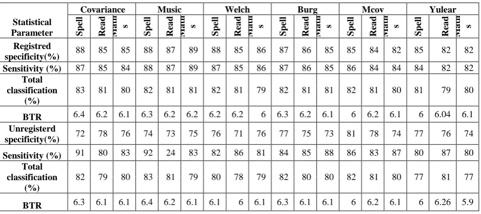
From the table1 it is observed that RNN model using burg algorithm has highest classification accuracy compared to static network model. It is also observed that the spell task is the most suitable among the three tasks studied. Predictive Power Analysis is used to measure recognition accuracy of the following tasks, namely read, relax, spell and math activity. True positive rate is called as sensitivity and false positive rate can be used to find the accuracy. True positive (TP) values are used to find the true detection of signals. False negative (FN) belongs to the signals, which remain undetected. False positive (FP) is false detected signal and True Negative (TN) is detected as a non event signal. Consider P as the total number of positive cases and N be the negative case. In predictive power analysis[16] the power spectral density using covariance algorithm obtained the accuracy of 83% for read and spell tasks.It had a bit transfer rate of 6.40 sec for registered subjects using the biometric system and the unregistered subjects show the maximum accuracy of 83%-77%. The bit transfer rate ranges from 6.42-5.99 sec. Power Spectral Density using modified Covariance, power spectral density using Pburg and power spectral density using yule-walker algorithm gave accuracy of 82% for spell task. The bit transfer rate obtained is 6.34 sec.

7. CONCLUSION

Recognition of EEG signal using RNN and FFNN is proposed in this study. EEG signals of 50 subjects is acquired non invasively using three. Best performance is achieved for the spell task with a mean accuracy of 95% using burg algorithm for RNN model. The experimental result shows that performances of the spell task using RNN model is better compared to FFNN model . Future works will involve the online testing of the signals and more dynamic network models will be used. Though this biometric system can be used only for small organizations, it can be used in high security level with limited individuals. It can identify individuals more precisely as compared to other currently used biometric systems.

8. REFERENCES

[1] Biometrics’ available online

http://en.wikipedia.org/wiki/Biometrics.

[2] C. Gope, N. Kehtarnavaz, and D. Nair. Neural network classification of EEG signals using time-frequency representation. In IEEE International Joint Conference on Neural Networks, volume 4, pages 2502 –2507, Montreal, Canada, 2005.

[3] P. Jahankhani, V. Kodogiannis, and K. Revett. EEG signal classification using wavelet feature extraction and neural networks. In IEEE John Vincent Atanasoff 2006 International Symposium on Modern Computing, pages 120 –124, Sofia, Bulgaria, 2006.

[4] Jian-Feng. Multifeature biometric system based on EEG signals. In Proceedings of the 2nd International Conference on Interaction Sciences, pages 1341–1345, Seoul, Korea, 2009.

[5] K. Ravi and R. Palaniappan. Leave-one-out authentication of persons using 40Hz EEG oscillations. The International Conference on Computer as a Tool, volume 2, Belgrade, Serbia& Montenegro, pp 1386 – 1389, 2005.

[6] R. Paranjape, J. Mahovsky, L. Benedicenti, and Z. Koles’. The electroencephalogram as a biometric. Canadian Conference on Electrical and Computer Engineering, volume 2, PP 1363 –1366, 2001.

[7] A. Riera, A. Soria-Frisch, M. Caparrini, C. Grau, and G. Rufﬁni. “Unobtrusive biometric system based on electroencephalogram analysis.EURASIP Journal on Advances in Signal Processing”, 2008:18, 2008.

[8] C.R. Hema, M. Paulraj, and H. Kaur. “Brain signatures: A modality for biometric authentication”. In International Conference on Electronic Design, pp 1– 4, Penang, Malaysia, 2008.

[9] M. Poulos, M. Rangoussi, V. Chrissikopoulos, and A. Evangelou. “Parametric person identiﬁcation from the EEG using computational geometry”. Volume 2, pp 1005 –1008, 1999.

[10]M. Poulos, M. Rangoussi, V. Chrissikopoulos, and A. Evangelou. “Person identiﬁcation based on the parametric processing of the EEG”. Volume 1, pp 283 – 286, 1999.

[11]K. Ravi and R. Palaniappan. “Leave-one-out authentication of persons using 40Hz EEG oscillations”. In The International Conference on Computer as a Tool, volume 2, pp 1386 –1389, 2005.

[12]Proakis JG, Manolakis DG. Digital Signal Processing Principles, Algorithms, and Applications. New Jersey, NJ, USA: Prentice-Hall, 1996.

[13]Kay SM, Marple SL. Spectrum analysis––A modern perspective. Proc of the IEEE 1981;69: 1380–1419. [14]Kay SM. Modern Spectral Estimation: Theory and

Application. New Jersey, NJ, USA: Prentice-Hall, 1988. [15]S.N.Sivanandam, M.Paulraj, Introduction to Artificial

Neural Networks Vikas Publishing House, India. 2003. [16]Arjon Turnip, Demi Soetraprawata, and Dwi E.

(6)

[image:6.595.74.527.92.445.2]

Table 1. Performance of the feed forward neural network and recurrent network for 50 subjects using four biometrics task

Table 2. Comparison of different feature extraction methods using RNN for EEG Signal classification

Statistical Parameter

Covariance Music Welch Burg Mcov Yulear

S

p

ell

Re

a

d

Ma

th _s

S

p

ell

Re

a

d

Ma

th _s

S

p

ell

Re

a

d

Ma

th _s

S

p

ell

Re

a

d

Ma

th _s

S

p

ell

Re

a

d

Ma

th _s

S

p

ell

Re

a

d

Ma

th _s

Registred

specificity(%) 88 85 85 88 87 89 88 85 86 87 86 85 85 84 82 85 82 82

Sensitivity (%) 87 85 84 88 87 89 87 85 86 87 86 85 86 84 84 84 82 82

Total classification

(%)

83 81 80 82 81 81 82 81 79 82 81 81 82 81 80 81 79 80

BTR 6.4 6.2 6.1 6.3 6.2 6.2 6.2 6.2 6 6.3 6.2 6.1 6 6.2 6.1 6 6.04 6.1 Unregisterd

specificity(%) 72 78 76 74 73 75 76 71 76 77 75 73 81 78 74 77 76 74

Sensitivity (%) 91 80 83 92 24 83 82 86 81 84 85 88 86 83 87 80 87 80

Total classification

(%)

82 79 80 83 81 79 80 78 79 82 80 80 82 81 80 77 81 77

BTR 6.3 6.1 6.1 6.4 6.2 6.1 6.1 6 6.1 6.3 6.1 6.1 6 6.2 6.1 6 6.26 5.9

Features Task

Recognition Accuracy of FFNN Recognition Accuracy of RNN

Max Min Mean SD Max Min Mean SD

PSD Using covariance algorithm

Relax 89 80 85 2.36 88 85 86.4 3.56

Spell 89 85 87.45 1.39 92 88 90 3.25

Maths 95 86 90.7 2.43 93 89 91.15 0.21

PSD Using burg algorithm

Relax 91 85 88.45 3.63 92 88 90 2.62

Spell 84 80 83.9 2.6 98 92 95 2.59

Maths 90 80 85.45 4.19 94 84 92 1.17

PSD Using modified covariance algorithm

Relax 83 80 83.3 3.77 90 88 89 2.44

Spell 90 80 85.45 3.97 91 87 89.9 2.45

Maths 92 83 87.15 3.79 95 89 92 3.67

PSD Using multiple signal classification

Relax 90 83 86.55 3.38 93 85 89 3.23

Spell 85 78 81.9 1.56 91 89 90.65 1.65

Maths 90 82 86 3.52 92 88 90 1.38

PSDUsing welch algorithm

Relax 87 78 82.8 2.34 95 83 89.9 1.28

Spell 92 83 87.6 2.96 90 88 89.6 2.61

Maths 89 85 87.5 3.35 91 83 91.2 3.75

PSD using yule walker algorithm

Relax 85 79 82 3.63 92 86 89 2.98

Spell 86 80 83 3.84 90 88 89 2.98

[image:6.595.66.535.473.682.2]