A methodology for developing resilient distributed control systems

(1)

A methodology for developing resilient distributed control

systems.

TAHOLAKIAN, Aram M.

Available from Sheffield Hallam University Research Archive (SHURA) at:

http://shura.shu.ac.uk/20418/

This document is the author deposited version. You are advised to consult the publisher's version if you wish to cite from it.

Published version

TAHOLAKIAN, Aram M. (1997). A methodology for developing resilient distributed control systems. Doctoral, Sheffield Hallam University (United Kingdom)..

Copyright and re-use policy

See http://shura.shu.ac.uk/information.html

(2)

Sheffield Hallam University

(3)

ProQuest Number: 10701064

INFORMATION TO ALL USERS

The quality of this reproduction is dependent upon the quality of the copy submitted.

In the unlikely event that the author did not send a com plete manuscript and there are missing pages, these will be noted. Also, if material had to be removed,

a note will indicate the deletion.

uest

ProQuest 10701064

Published by ProQuest LLC(2017). Copyright of the Dissertation is held by the Author.

This work is protected against unauthorized copying under Title 17, United States C ode Microform Edition © ProQuest LLC.

ProQuest LLC.

789 East Eisenhower Parkway P.O. Box 1346

(4)

A Methodology for Developing

Resilient Distributed Control Systems

Aram Meguerditch Taholakian BEng

(Hons)

A thesis submitted in partial fulfilment of the

requirements of Sheffield Hallam University for the degree of

Doctor of Philosophy

(5)

Abstract

Manufacturing industries rely on automated manufacturing systems to improve the

efficiency, quality and flexibility of production. Such systems typically consist of a variety of manufacturing machinery and control hardware, e.g. CNC machine tools, robots, PCs,

Programmable Logic Controllers (PLCs) etc., which operate concurrently. The cost of developing and implementing an automated manufacturing system is high, and is particularly so if the control system is found to be unreliable or unsafe during operation. Distributed Control Systems are generally used to control complex concurrent systems, At present the methods used to develop DCSs tend to follow a sequence of steps, viz. a statement of the requirements of the DCS, a functional specification of the DCS, the design of the DCS, generation of the software code for the DCS, implementation of the software. This step approach is inadequate because of the dissimilarity of techniques used to represent each step, which leads to difficulties in ensuring equivalence between the final

implementation of the DCS and the initial requirements, which in turn leads to errors in the final software. To overcome this, work has been conducted to unify the specification, design, and software coding phases of the DCS development procedure by ensuring formal

equivalencies between them. One particular outcome of such previous work is a tool named Petri Net - Occam Methodology, developed by Dr. P. Gray, which produces dependable Occam code for DCSs. Gray’s methodology produces readable designs, directly from the specification of systems, in a graphical but formal way, and results in a Petri Net graph which is equivalent to the final Occam code. However, his methodology is not for a complete DCS but only for one containing Transputers.

The PLC is widely used in industry and an integral part of DCSs for Automated Manufacture. This research has developed a methodology, named PN<=>PLC, which produces dependable PLC control programs, in a graphical but formal way, directly from a system’s specification. It uses the same tool, Petri Nets, for both designing and simulating the control system, and specifies rules which ensure the correct design, simulation and encoding of PLC programs. The PN designs are a one-to-one equivalent to PLC code and can be directly translated into Ladder Diagrams. Therefore if the simulation shows the design to be correct, the final software will be correct.

PN<=>PLC works as a stand alone tool for developing dependable PLC control programs, and also unifies with Gray’s methodology to produce a complete tool for developing a resilient DCS containing Transputers and PLCs. The unification of the two methodologies is also reported in this thesis.

(6)

List of Figures

Figure 2-1 Layout of the FMC at the School of Engineering...13

Figure 2-2 Levels of Control of the FM C...14

Figure 2-3 The Labyrinth PN Graph of the FM C...inside back cover Figure 2-4(a) A Simple Petri Net... 19

Figure 2-4(b) A Marked Petri Net...20

Figure 2-4(c) Marking After the Firing of the Transition... 20

Figure 2-4(d) Inhibitor Arc PN Graph Showing the Marking Before and After the Firing of the Transition... 21

Figure 2-5 Gray’sPN Graph for the Control of the FM C inside back cover Figure 3-1 Oil Tank Level...38

Figure 3-2 PN Graph of Oil Tank Level Control Produced By Gray’s Methodology... ...38

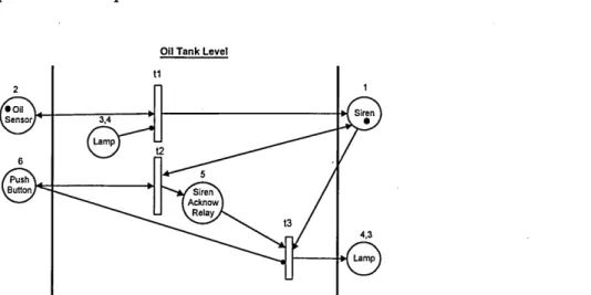
Figure 3-2(a) Marking Achieved as a Result of Simulating Oil Sensor Switching on... 39

Figure 3-2(b) Marking Achieved as a Result of Simulating Push Button Being Pressed...40

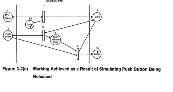
Figure 3-2(c) Marking Achieved as a Result of Simulating Push Button Being Released ...40

Figure 3-2(d) Marking Achieved as a Result of Simulating Oil Sensor Switching off...41

Figure 4-1 Layout of PN<=>PLC Graph...47

Figure 4-2(a) First Design Rule Applied to Siren... 48

Figure 4-2(b) Second Design Rule Applied to Siren...49

(10)

Figure 4-2(bl) A Realistic Marking Applied to Figure 4-2(b)...50

Figure 4-2(b2) Evolution of the Marking After Applying Simulation Step 3 to Figure 4-2(bl)... 50

Figure 4-2(c) Design Rules Applied to Siren and Lamp... 51

Figure 4-2(d) Final PN<=>PLC Graph of Oil Tank Level Control...52

Figure 4-3(a) LD Showing the Conditions for Switching the Siren on. First Translation Rule...54

Figure 4-3(b) LD Showing How the Siren is Latched on. Second Translation Rule... 55

Figure 4-3(c) LD Showing the Conditions for Switching the Siren off. Third Translation Rule...55

Figure 4-3(d) Final LD. An Exact Behavioural Equivalent to the PN<=>PLC Graph Shown in Figure 4-2(d)...56

Figure 4-4(a) Initial Marking Representing the Oil Sensor Switching on, i.e. Scenario 1, Event (a). Simulation Step 2... 58

Figure 4-4(b) Evolution of Marking After Applying Simulation Step 3 to Figure 4- 4(a)...58

Figure 4-4(c) Marking which Represents Scenario 1, Event (b)...60

Figure 4(d) Evolution of Marking After Applying Simulation Steps to Figure 4-4(c)...60

Figure 4-4(e) Marking which Represents Scenario 1, Event (c)...60

Figure 4(1) Evolution of Marking After Applying Simulation Steps to Figure 4-4(e)... 60

Figure 4-4(g) Marking which Represents Scenario 1, Event (d)...61

Figure 4(h) Evolution of Marking After Applying Simulation Steps to Figure 4-4(g)...61

(11)

Figure 5(b) Evolution of Marking After Applying Simulation Steps to Figure

4-5(a)... 62

Figure 4-5(c) Marking which Represents Scenario 2, Event (b)...62

Figure 5(d) Evolution of Marking After Applying Simulation Steps to Figure 4-5(c)... 62

Figure 4-5(e) Marking which Represents Scenario 2, Event (c)...63

Figure 5(f) Evolution of Marking After Applying Simulation Steps to Figure 4-5(e)... 63

Figure 4-5(g) Marking which Represents Scenario 2, Event (d)...63

Figure 5(h) Evolution of Marking After Applying Simulation Steps to Figure 4-5(g)... ... 63

Figure 4-6 Petri Net Graph of Oil Tank Level Control... 65

Figure 4-6(a) Evolution of the Marking After Simulating Scenario 1, Event (a) 66 Figure 4-6(b) Evolution of the Marking After Simulating Scenario 1, Event (b) 66 Figure 4-6(c) Evolution of the Marking After Simulating Scenario 1, Event (c). 67 Figure 4-6(d) Evolution of the Marking After Simulating Scenario 1, Event (d) 67 Figure 4-7(a) &Figure 4-7(b) Two Possible LD Interpretations of the PN Graph Shown in Figure 4-6...70

Figure 4-8 Design of Oil Tank Level Control Using SFCs... 71

Figure 4-9 LD Translation of the SFC in Figure 4-8...71

Figure 5-1 Initial Error Checks Performed Using a ‘pulse’... 77

Figure 5-2 PN Graph Showing the Use of a ‘group signal’... 78

Figure 5-3 PN Group Containing Initial Error Checks...80

Figure 5-4 PN Group Showing an Alternative Error Check... 81

Figure 5-8 A PN Group Showing the Use of a Timer...82

(12)

Figure 5-13 Ladder Diagram Translation of ‘Milling PN Graph’... 87

Figure 5-14 A Ladder Diagram Equivalent to Figure 5-13...87

Figure 5-15 Enable Vice to Table PN Step... 89

Figure 5-15L Step Diagram Translation of Figure 5-15... 91

Figure 5-24 Puma Station Error Status PN Graph ... 99

Figure 5-23 Puma Station Complete Status PN Graph... 101

Figure 6-1 A PN Graph Showing the Unification of PN<=>rLC with Gray’s

(13)

Dedication

I wish to dedicate this thesis to all my family, especially my father and my mother for

their moral and financial support throughout my studies.

I also wish to dedicate this thesis to my partner for her support and patience,

particularly throughout the writing-up period.

Acknowledgments

I would like to express my sincere gratitude to my director of studies, Dr W M M

Hales, for his excellent supervision and support. I would also like to thank my

supervisor, Prof F Poole, Mrs J Grove, Mr G Cockerham and Prof E Lo for their

support and advice.

Thanks also to all technicians involved, colleagues and friends.

Declaration

I declare while registered as a candidate for the University’s research degree, I have

not been a registered candidate or enrolled student for another award of the University

or other academic or professional organisation. I further declare that no material

contained in this thesis has been used in any other submission for an academic award.

(14)

Chapter 1 Introduction

1. Introduction

This chapter gives a brief introduction to Distributed Control Systems (DCSs), mainly

Flexible Manufacturing Cells, and discusses the current approaches used to develop

the various parts of a DCS. The introduction then concludes by identifying a need for

a methodology for developing a dependable DCS, such that the methodology is

applicable to all aspects of the DCS, and not just the higher levels or the lower levels,

in a formal but readable way.

1.1 Automated Manufacture

Manufacturing industries employ a wide range of technologies in their processes to

improve their competitive strength in the market place. Recent advancements in

information technology have produced fully automated, efficient but complex

manufacturing systems. Programmable automation tools, such as Programmable

Logic Controllers (PLCs), Robots and computer numerical control (CNC) machines,

are used to increase the efficiency and quality of manufacturing plants. Automated

Manufacturing Systems offer numerous advantages such as short lead-times, low

work-in-progress, reduced labour and hence reduced unit costs, and quick change-over

times. They also provide flexibility which enables rapid responsiveness to market

changes.

1.1.1 Flexible Manufacturing

The ability to meet customer demands and remain in touch with an ever increasing

competitive market place [Ford 1991] has resulted in manufacturing industries

(16)

Chapter 1

(FMCs) have been well established for a number of years [Narahari and

Viswanadham 1986, Huang and Chang 1992, Lu and Huang 1992, Chao et al 1992]

and are used in batch manufacturing industries to improve the efficiency of

production. They consist of a number of CNC machine tools, automated work/tool

handling equipment and a control system to synchronise the operation of the machine

tools and handling equipment. The integration and coordination of a group of FMCs

produces a larger flexible manufacturing environment often referred to as a Flexible

Manufacturing System (FMS) [Simpson et al 1982, Ayers 1988]. FMSs can be used

to produce complex products, where individual components are made in various

FMCs and then assembled in a Flexible Assembly System (FAS) [Williams and Lill

1987].

The safe and reliable operation of Flexible Manufacturing Cells is clearly desirable, if

not essential for their effective use. However FMCs are complex systems the

elements of which operate concurrently, and interact at irregular times depending

upon the components to be produced. Therefore the development of a control system

is not a trivial affair [Slack 1988, Duan and Kumara 1993]. Control systems not only

consist of computer algorithms, but also computer hardware, communications

protocols and cell monitoring equipment, such as sensors and transducers.

1.2 Distributed Control Systems

Some automation tasks are simple to achieve, whereas others, for example FMCs, are

far from simple, because they consist of a number of autonomous devices which

operate concurrently, but also in synchronisation with each other.

(17)

Chapter 1

and is particularly so if the design is found to be unreliable during or after

implementation.

Controlling complex concurrent systems is only feasible if the task of control is

distributed amongst a number of devices (section 2.1.2). Flexible manufacturing

operational strategies such as Distributed Control are now established practices in

industry. Real time control is achieved by distributing the various functions of a

control system which operate concurrently. It is essential however that these functions

or elements communicate with each other to achieve complete synchronisation of the

whole system. Such communication could be achieved by networking individual PCs,

which each run sequential programs. However as the number of processors increases,

the management overhead increases [Das and Fay Freund 1983].

The programming strategies and languages available for conventional

microprocessors do not model a parallel architecture [Naghdy and Strickland 1989].

Apart from developing the program for each processor separately from others, the

programmer has to introduce techniques for synchronisation and communication of

one processor with others. However the software is directly dependent on the

hardware. By increasing the number of processors, the complexity of the software

design, development and testing will multiply. Expansion or modification of the

operation of the hardware requires major modification of the software.

In recent years, systems specific processors and software have been developed to

overcome the above mentioned problems. For example, the combination of the

Transputer (a microprocessor, see section 2.2.1) and its programming language

(18)

Chapter 1

various industries for embedded systems, numerical analysis, image processing and

Real-Time Distributed Control Systems.

1.3 Development of Distributed Control Software

At present the methods used to develop Distributed Control Systems tend to follow a

sequence of steps:

• Statement of requirements of the DCS

• Statement of the functional specification of the DCS

• Design of the DCS to meet the specification

• Generation of the software code for the DCS

• Implementation of the software

It is widely acknowledged that this method has its drawbacks [Shatz and Wang 1987,

Boehm 1988, Jelly and Gorton 1994]. The requirements and specification are usually

written in English, the design may be depicted graphically or textually, and the

software usually written in a high level language. This leads to difficulties in ensuring

equivalence between the final implementation of the DCS and the initial requirements,

because of the dissimilarity of techniques used to represent the steps, and the

differences in the expertise of those who develop each step. The development of one

step is a translation of the previous step, thus there is no reliable isomorphism between

the steps. Practitioners attempt to ensure equivalence between the various steps by

checking the equivalence of each step with its preceding step. Some methods used to

do this are formalised, and some are ad hoc; none are totally satisfactory [Bloomfield

(19)

Chapter 1

To improve on this method of developing DCSs, equivalence of representation is

required at each step. The ideal way to achieve this would be to develop a

methodology which uses the same language, one that all parties could understand, at

each stage of the development, and could be verified against the system requirements

prior to implementation.

1.3.1 Informal Methods for Designing DCSs

Distributed Control Systems are often categorised into more than one level of control.

For example the control of an FMC may be divided into several levels ranging from

the Programmable Logic Controller (PLC) operated sensor and actuator control level,

to a high decision making level, often referred to as the Cell Controller (CC) level.

A considerable amount of research into the different levels of DCSs has been recently

carried out by various parties. For example, many have attempted to develop

alternative PLC program representations (discussed further in Chapter 2, section 2.4).

For the most part, these attempts have focused, not only on the lowest level of a DCS,

but also on a particular aspect of the software development process, mainly modelling.

There have also been attempts to use Petri Nets (PNs) to design PLC programs, but

virtually all the resulting PN models pay scant regard to the readability [Taholakian

and Hales 1995], which severely restricts their practical applications: a design which

is unclear to read is difficult to check for correctness, difficult to maintain and

difficult to update, i.e. it is unreliable.

1.3.2 Formal Methods for Designing DCSs

Extensive research has also been carried out into the higher levels of DCSs. For over a

(20)

unapter i

Weston has researched into areas such as Computer Integrated Manufacture (CIM)

and has produced computerised systems for developing CIM systems [Weston 1991,

Weston 1993], namely CIM-BIOSYS, which is an infrastructure designed to integrate

the various software applications needed to achieve highly autonomous and flexible

CIM systems. The group has also investigated the behavioural modelling of CIM

systems using techniques such as CIM-OSA and Stochastic Timed Petri Nets

[ESPRIT/AMICE 1991, Aguiar and Weston 1993], and of late has investigated the

use of PNs to design code for DCSs [Ariffin et al 1995].

A large amount of research has been carried out by various parties into the use of Petri

Nets for modelling and performance evaluation of DCSs: [Kamath and Viswanadham

1986, Huang and Chang 1992, Viswanadham and Narahari 1992, Barkaoui and Ben

Abdallah 1993* Hilal and Ladet 1993, Reddy et al 1993]. Numerous publications

referring to the use of PNs for the detection of faults, specifically “deadlock”, are also

widely accessible [Murata and Shenker 1989, Viswanadham et al 1990, Ezpeleta et al

1995].

A group of academics and researchers at Sheffield University has worked on

automatically producing software from a system specification, for implementation on

a parallel platform consisting of Transputers and C40s [Bass et al 1994]. Others have

also investigated the implications of Transputers and Parallel Processing for DCSs

[Draper and Holding 1989, Tudruj 1992, Lau and Seet 1993, Sundaram and Narahari

1993, Moore and O’Donoghue 1994].

At the School of Engineering (SOE), Sheffield Hallam University, there is ongoing

(21)

Chapter 1

reports on a PN-Occam based methodology for developing DCSs (Chapter 2, section

2.2.3). Gray’s methodology pays strict attention to the readability and

comprehensibility of the design. Gray claims that the design translates, with exact

equivalence, into the Occam programming language to run on Transputers. He also

claims that it is expandable and avoids control errors such as “deadlock” from being

introduced into the code. However Gray’s methodology has only been applied to

Transputers and Occam, which is only part of an overall DCS. More than often DCSs

in manufacturing industries consist of more than one type of controller. The PLC is

widely used in industry (section 2.3), in conjunction with other controllers such as

PCs and Transputers, to achieve Distributed Control. There is no evidence whether

his methodology is applicable to such an overall DCS.

1.4 The Need for a Methodology for Developing DCSs

From the preceding discussion it is apparent that the current methods for developing

distributed control software do not ensure dependability of the system. Although

work has been done on designing parts of DCSs, there is no methodology for ensuring

that an overall DCS is dependable and meets the requirements.

A need has been identified for a methodology for designing DCSs such that:

• the methodology is easy to understand and of practical use in industry.

• the methodology is applicable to all aspects of a DCS and not just the higher

levels or the lower levels.

(22)

Chapter 1

• the design is represented in a readable format which enables parties other than just

the original designer to understand the design and thus reliably check for

correctness, reliably maintain and expand the system.

• the designer is guided towards designing an error free control system prior to

implementation.

• the design is modular to allow flexibility of the DCS.

• the design is graphical but formal and supports simulation thus eliminating the

need to translate the design into an independent simulation software to analyse.

• the design is equivalent to the control algorithm, i.e. there are formal rules for

translating the design into the final control code to ensure that the two operate in

exactly the same way. Thus if the design is correct, then the control code will be

(23)

Chapter 2 Background

2. Background

This chapter describes the Flexible Manufacturing Cell at the School of Engineering

which was used as the test bed for the reported research project. It discusses the

control and the communication between the various levels of the control. The chapter

also introduces Petri Nets and a Petri Net - Occam methodology, which was the

outcome of previous research carried out at Sheffield Hallam University’s School of

Engineering. The incompleteness of previous approaches, including the Petri Net -

Occam methodology, are discussed, and in particular their inapplicability to low level

PLC control. The PLC is an integral part of an FMC, and in this chapter the

inadequacies of existing PLC programming strategies are also discussed. A need for a

methodology for developing PLC based DCSs is identified. Finally the aims and the

objectives of the PhD research are stated.

2.1 The FMC at the School of Engineering

Gray’s Petri Net - Occam methodology was the initial motivation for this research

project. The Flexible Manufacturing Cell (FMC) at the School of Engineering (SOE),

Sheffield Hallam University, was chosen for the development and testing of both

Gray’s methodology and the reported Ph.D. research. It is therefore appropriate to

describe the FMC prior to explaining Gray’s methodology.

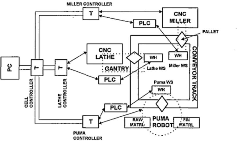
The FMC consists of a CNC lathe, CNC milling machine, a conveyor track, and three

work stations (WS) as follows:

□ Puma WS for loading and unloading raw material and finished parts.

(26)

Chapter 2

□ Miller WS for loading and unloading the miller.

The loading and unloading of raw materials and finished parts is carried out by a six

axis, programmable Puma robot. The loading and unloading of the lathe is carried out

by a pneumatically operated gantry robot, while a pneumatic cylinder loads and

unloads the miller by ramming a workpiece to and from a fixture on the milling table.

A conveyor track transports components to and from the work stations. This

equipment is referred to as the work handling (WH) equipment (Figure 2-1, below).

Chess pieces designed for blind players are the chosen components for the cell. This

introduces flexibility into the cell for the following reasons:

1. Different machining processes are employed to produce the pieces, which are in

turn machined differently to distinguish the two colours by touch.

2. Chess sets of different dimensions or styles can be produced.

MILLER CONTROLLER

MILLER

LATHE

Miller WS

GANTRY Lathe WS

P u m a WS

•FIN

ROBOT! MATRL PUMA

CONTROLLER

(27)

Chapter 2

2.1.1 Levels of Control

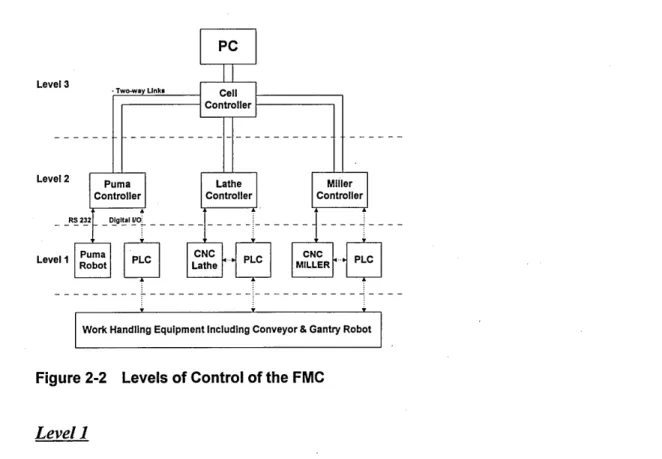
The equipment used to perform the logical control of all the elements within the FMC

is distributed between Transputers and PLCs (Programmable Logic Controllers), and

divided into three levels of control, as shown in Figure 2-2.

Level 3 _{♦ T w o -w ay Link»}

Level 2

D igital J/O j

Level 1 Pum a_{R obot} PLC _{L athe}CNC PLC _MILLERCNC PLC Cell

C o ntroller

L athe

C o ntroller C ontrollerMiller PC

P um a C on tro ller

W ork H andling E q u ip m en t Including C o n v ey o r & G antry R obot

Figure 2-2 Levels of Control of the FMC

Level 1

The simple sequential control of primitive devices, such as actuators and sensors, is

carried out in Level 1 using PLCs.

One PLC is devoted to the Puma WS. The opening of the dogs on the conveyor,

closing them when the pallets have moved on, and the monitoring of the appropriate

sensors at the Puma WS, to determine the arrival/departure of pallets at/from the

station, is carried out through this PLC.

A second PLC is devoted to the Miller WS. It monitors the appropriate sensors at the

(28)

V s M c i|J ie i £

cylinder, the milling fixture clamp and instructs the miller to start or stop machining.

The PLC also monitors the machining status of the Miller.

A third PLC is used to control and monitor the Lathe WS and the gantry robot,

synchronising the opening and shutting of the lathe door with the entry and exit of the

robot arm whilst loading and unloading workpieces. The execution of the “Start

Machining” command to the Lathe, and the monitoring of the machining status is also

carried out through this PLC.

Level 2

The control of the machine tools, robots and the PLCs conducting Level 1 control is

achieved in this level.

The Puma Transputer, for example, instructs the Puma robot to execute the program

“Load Cell”, which is used to place a blank from the raw material stock in a vice on a

pallet. It also instructs the PLC at the Puma WS to convey pallets between work

stations.

The Miller Transputer, for example, instructs the PLC at the Miller WS to transfer the

vice into the fixture on the milling table and clamp it in place.

The Lathe Transputer instructs the PLC at the Lathe WS to operate the gantry robot,

to load or unload the lathe, and to monitor the arrival of pallets and the opening and

closing of their vice accordingly.

Level 3

Level 3 is conducted by the Cell Controller. The Cell Controller's task is to ensure

(29)

Chapter 2

instructions to the Level 2 controllers to load and unload the machine tools, to start

machining cycles and convey parts round the cell.

2.1.2 Reasons for Distributing Control

Having established that the control of the School of Engineering’s cell is achieved by

distributed control, it is important to explain the reasons behind such a design. Why,

for instance, is the whole cell not controlled by only one computer.

Two essential reasons:

1. To reduce the complexity of the control algorithms/computer programs.

Even with the small FMC at the SOE., the number of sensors that need monitoring,

and the number of actuators which need operating is very large. Since the various

parts of the cell operate concurrently, the control of such an environment by one

sequential algorithm becomes virtually impossible, and certainly inefficient. Changes

within the cell would mean redesigning the complete control algorithm, hence making

future growth a very difficult task. An example of concurrency within the cell could

be, when a part is to be unloaded from the conveyor by the Puma robot, also a part is

to be loaded onto the miller and whilst this is being carried out, the lathe finishes

machining and requires its workpiece to be removed.

2. To achieve the required communications necessary to operate the machine tools

and work handling equipment.

There are several types of data that have to be communicated within the cell. For

example, whether a sensor is on or off, which program the Puma is to run, what

component is to arrive at the Miller. This data is communicated in different ways

(30)

U l l d ( J l C I £.

off (24 or 0 volts) and requires only two wires to transmit its data. However, more

complex messages have to be passed between station controllers and the machine

tools, e.g. to instruct the Puma to run a certain program requires the Puma station

controller to transmit the command “EXEC LOADPART”, and the Puma to reply

“PART LOADED”. RS 232C is used to handle this duplex communication.

Messages which pass between the Cell Controller and the station controllers may be

transmitted simultaneously, therefore a Local Area Network (LAN) having a multiple

access communication protocol is used. A single control algorithm to handle all these

communications in Real-Time would be difficult or perhaps impossible to write.

2.2 Gray’s Petri Net - Occam Methodology

Over the years, Petri Nets (section 2.2.2) have been used in modelling safety critical

systems to reduce faults in the system by removing them before use [Sahraoui et al

1987, Leveson and Stolzy 1987, Viswanadham and Johnson 1988, Reddy et al 1993].

FMCs are a particular case of safety critical systems in that, although automated they

work in conjunction with humans.

Gray conducted research to show that Occam and Transputers could considerably

simplify the design of DCSs for FMCs. He chose to use Petri Nets as the formal

method for developing DCSs, but soon found that Petri Net graphs can become very

complex (Figure 2-3, inside back cover). The graph is not readable and difficult to

follow.

For these reasons and inspired by the capabilities of Occam and Petri Nets, Gray

developed a methodology for producing dependable distributed control software for

(31)

Chapter 2

It is important however to discuss Transputers, Occam and Petri Nets, in more detail,

for a better understanding of the methodology.

2.2.1 Transputers and Occam

The combination of the Inmos developed hardware and software called Transputer

and Occam respectively has now been recognised as a solution to the problem of

programming concurrent systems.

A Transputer is a microcomputer with its own local memory, and with

communication links for connecting one Transputer to another Transputer [Inmos Ltd.

1990]. The protocols for communications between Transputers is built into the

hardware of the Transputer chip. It can be used in a single processor system, or in

networks to build high performance parallel architectures. By linking processors

together, a linear increase in data processing capacity can be achieved, as opposed to

the limited processing capacity of typical multi-processor control systems (MPCS). A

MPCS can only be increased to a certain limit before experiencing a drop off in

effective computing power [De Gaspari 1992].

2.2.1.1 Occam: Language Definition

Occam simplifies the writing of concurrent programs by taking most of the burden of

synchronisation away from the programmer [Inmos Ltd. 1989]. Occam uses channels

for communicating values and does not distinguish between two processes (programs)

running concurrently on different computers, or concurrently on the same computer.

However channels are one-way only, and therefore two are needed for a two-way

(32)

Although Occam provides synchronised communication, the programmer is still left

with the responsibility of avoiding “deadlock”, i.e. a process waiting for

communication that will never arrive, for it is prepared to do so forever . For the non

professional programmer, or rather the professional engineer and system designer,

avoiding deadlock, in even a relatively simple FMC such as the one in the School of

Engineering, is difficult.

2.2.2 Introduction to Petri Nets

Petri Nets are a tool for the study of systems, and a graphical representation of

systems [Peterson 1981]. In 1962 Carl Adam Petri, a German mathematician defined

Petri Nets as a mathematical modelling tool for describing relations between

conditions and events, whether sequential or concurrent. The basics of Petri Net

graphs are as follows:

Places. Transitions and Arcs

A place is represented by a circle and a transition is represented by a bar or a box.

Places and transitions are connected by arcs (Figure 2-4(a), below). An arc is

directed and connects either a place to a transition or a transition to a place. Arcs

directed from a place to a transition define the place to be an input of the transition.

Arcs directed from a transition to a place define the place to be an output of the

transition. Thus in Figure 2-4(a) A, B and C are input places to transition tl, and D

and E are output places of tl.

(33)

Chapter 2

Markins

Marking is the assignment of tokens or marks to the places of a PN (Figure 2-4(b),

below). A token is represented by a dot in a place. The marking at a certain moment

defines the state of the system described by the PN. In Figure 2-4(b) the input places

A, B and C are said to be active. Places can also be ‘bounded’, which means there is a

limit on the maximum number of tokens a place can hold. e.g. a place bounded to one

token can only contain one token at any one time.

Figure 2-4(b) A Marked Petri Net

Fir ins of Transitions

A transition can only be fired if each of its input places has at least one token. The

transition is then said to be fireable or enabled (Figure 2-4(b), above). Firing of a

transition consists of withdrawing a token from each of its input places and adding a

token to each of its output places (Figure 2-4(c), below). The firing of a transition is

indivisible (has zero duration), except when considering Timed or Synchronised PNs

(34)

U l l d p i m £.

Inhibitor Arcs

An inhibitor arc is a directed arc which joins a place to a transition. However its end

is marked with a small circle (Figure 2-4(d), below). The inhibitor arc between the

input place C and the transition means that the transition is only enabled if the place C

does not contain a token, as shown in Figure 2-4(d).

Before Firing After Firing

Figure 2-4(d) Inhibitor Arc PN Graph Showing the Marking Before and After the Firing of the Transition

The above is not a definitive description of PNs, but is sufficient for understanding the

methodology.

2.2.2.1 High Level Petri Nets

High level Petri Nets are folded versions of the general Petri Nets described above.

Unfolding a high level Petri Net produces a set of places, where one place was, and a

set of transitions, where one transition was. Folding a general Petri Net into a high

level one is the reverse of this. The way in which general and high level Petri Nets are

read is different. In reading general Petri Nets more emphasis is given to places and

transition rather than tokens and arcs; “WIZIWIG, what you see is what you get”. In

high level Petri Nets more emphasis is given to reading tokens and arcs rather than

places and transitions, due to some, if not most, of the information being folded away.

(35)

Chapter 2

2.2.3 The Motivation and Objectives of Gray’s Methodology

Gray highlighted the need of a novel methodology in three stages as follows:

a) The needs of a Transputer based FMC

b) The needs of an Occam based methodology

c) The use of Petri Nets with Occam

A verification of these needs and a full criticism of current use of Petri Nets and

Occam is given in his thesis [Gray 1995]. Gray’s conclusion of these needs are drawn

from the suitability of Transputers and Occam as the hardware and software for the

control of a DCS, the lack of sufficient guidance in the development of flexible and

dependable Occam code, and the applicability of Petri Nets to DCSs and their

popularity in the manufacturing field.

In addition to the references to the lack of adequate guidance provided by other

existing Petri Net-Occam techniques, Gray highlights other significant disadvantages

associated with current practices, mainly the following:

1. The most common approach of developing Petri Net models is informal, i.e.

produce a Petri Net graph and analyse it. When the model is found to be incorrect,

it is then modified and re-analysed. This may be repeated several times before an

accurate model is achieved.

2. High level Petri Net graphs are often used because they are graphically more

concise than their equivalent general Petri Net graphs, but the information held

(36)

ir n a p ie r £.

3. Even general Petri Net graphs are almost always found to be very difficult to read,

and thus understand, because they are drawn in an unstructured fashion (Figure 2-

3, inside back cover).

4. Occam code refinement is tedious. The conventional approach of developing

Occam code is to draft its basic structure using DFDs or PNs, produce the Occam

code and try and compile it. If and when it does not compile, it is then modified

and re-compiled. This process is repeated until successful.

5. Using formal design techniques will help produce reliable and safe control

systems. However, a tedious development process is often involved in using

formal methods and mathematicians are required to design and verify the control

programs. This is costly both in time and in wages, and therefore industry is

reluctant to use such methods.

Having discussed the problems associated with existing DCS development methods

and techniques, Gray concludes that there is a need for a methodology which makes

better use of Petri Nets and Occam. The aims and objectives of his novel

methodology can be summarised as follows:

• to produce the specification of the DCS directly from the manufacturing

requirements.

• to produce the specification in a graphical but formal way, which will be

comprehensible during all stages of the development life cycle of the FMC, i.e.

specification, design, simulation, coding, implementation and maintenance.

• to obtain equivalence between the model and the code by exploiting the

(37)

Chapter 2

• to incorporate “deadlock” prevention into the methodology by having a

unidirectional communication protocol.

• to produce dependable Occam code to run on a network of Transputers for the

control of an FMC.

2.2.4 Gray’s Methodology Applied to the FMC

To achieve the aims and objectives listed above in section 2.2.3, Gray’s methodology

consists of four design steps and employs certain techniques which play a key role in

the development of dependable DCSs. For example, “deadlock” is avoided by

employing a technique that Gray calls “output-work-backwards” and a uni-directional

flow of information between the various controllers of the FMC. Where two way

communication is required between controllers, for example between the Cell

Controller and the Status Handler (Figure 2-5, inside back cover), then a client-server

relationship between the two is employed (discussed below).

The four steps of the methodology are:

Step 1 Identify concurrent and sequential operations.

Step 2 Produce a Petri Net graph for each controller.

Step 3 Combine the controller Petri Net graphs.

Step 4 Translate the Petri Net graphs into Occam code.

Each step consists of one or more tasks, as described below.

The task in step 1 is to analyse the overall concurrency of the FMC. Some operations,

such as the lathe and the miller machining at the same time, are stated in the

(38)

u n a p ie r c

are independent, for example lathe machining and the conveyor indexing. Most

sequential operations are also obvious, e.g. loading the lathe before machining, or

loading a part into a pallet before indexing (transporting) the part to the lathe. The

need for a Cell Controller (CC) and a Status Handler (SH) is also identified during

this step. The hierarchical nature of the manufacturing control system and the master-

slave method of communication often used in Transputer networks [Gray 1995]

prompts the need for a cell supervisor or master to the slave work station controllers.

The Status Handler is slave to the work station controllers but operates as a server to

the client Cell Controller. The task of the Status Handler is to prevent “deadlock” by

gathering feedback from the work station controllers, and acts as a buffer between the

Cell Controller and the rest of the cell. The communication between the Status

Handler and the Cell Controller is controlled, to avoid “deadlock”. The Status

Handler will not communicate with the Cell Controller unless the Cell Controller

requests an update for the status of the cell.

The tasks involved in step 2 are to examine the requirements of the controllers and

design the logic of the individual controllers. Petri Net graphs for each controller are

produced, which clearly list the inputs to the controllers, the logical operation of the

controllers and the outputs from the controllers. Where the inputs come from and

where the outputs go to, are also clearly stated during this step. Gray prescribes a

specific format for drafting PN graphs, to ensure that they are readable.

Step 3 is concerned with integrating the individual controller PN graphs to produce an

overall PN graph, which is the specification of the DCS. Managing the

(39)

Chapter 2

The task in step 4 is that of translating the Petri Net graph into Occam. The rules of

the methodology ensure that the overall PN graph is equivalent to the Occam

constructs, making the translation process reliable, efficient and relatively simple.

By following these steps, the overall PN graph for the control of the FMC described

in section 2.1 was produced (Figure 2-5, inside back cover).

2.2.5 Advantages, Disadvantages and Claims of Gray’s Methodology

Gray’s objectives for his methodology are worthwhile; he achieves a readable,

modular and dependable design which can be checked for correctness, and translated

reliably into control software. However, his methodology could not be used to design

a complete DCS which consists of controllers other than Transputers. In particular,

Gray does not consider PLCs which are very commonly used in industry worldwide.

Indeed PLCs are an integral part of the FMC chosen by Gray for the development of

his Petri Net - Occam methodology. Nevertheless, Gray claims that his methodology

produces a design which can be both reliably updated and expanded. These claims

were investigated as part of the research programme and are discussed in Chapter 6.

2.3 Programmable Logic Controllers

The PLC is a microcomputer which evolved from the conventional computers of the

late 1960s and early 1970s [Webb 1992]. Over the last twenty years the PLC has

become an integral part of industrial control systems due to its rugged structure and

high processing capabilities. The basic structure of the PLC consists of a Central

Processing Unit (CPU) and input/output modules or terminals. Increased technology

has made it possible to cram more functions such as numerous relays, timers and

(40)

V srictpiei £.

output signal from the PLC (I/Os) can be either 24 volts or 0 volts (section 2.3.1.5),

and are used to control a wide range of devices such as solenoids, actuators and

robots.

2.3.1 Available PLC Programming Tools and Techniques

One of the major restrictions to new PLC concepts being applied in industry is the

difficulty to change the desire of some users to use Ladders Diagrams [Webb 1992].

In fact, the Ladder Diagram approach of PLC programming, based on conventional

'relay logic', still remains the most commonly used technique employed by the vast

majority of industries in the UK and the USA [Jafari and Boucher 1994]. A decade

ago S. M. Cotter [Cotter and Woodward 1986] wrote: "Like it or not, then, the ladder

diagram is likely to be with us for some years yet." This still holds true today despite

the definition of other PLC languages in the IEC 1131-3 standard [IEC 1992] by the

International Electrotechnical Commission. The standard suggests five languages for

programming PLCs; Instruction List (IL), Structured Text (ST), Function Block

Diagram (FBD), Sequential Function Chart (SFC) and finally Ladder Diagram (LD).

However none of the five suggested languages are design methodologies, nor are they

widely accepted or tested, with the exception of Ladder Diagrams.

2.3.1.1 Instruction List

Instruction List is a textual low level language, similar to an assembler language,

without support for structuring. An Instruction List consists of a sequence of

instructions or operations, with each instruction beginning on a new line. It is useful

(41)

Chapter 2

2.3.1.2 Structured Text

Structured Text, as its name implies, is a structured textual high level language, which

has a similar syntax to the programming language PASCAL. Structured Text can be

used to create application specific function blocks. Complex statements involving

variables which represent a wide range of data types (including analogue and digital)

can be expressed using ST. It also supports types of data specific to batch processing

applications, such as time, date and duration. In addition, ST supports iteration loops

such as REPEAT UNTIL, conditional execution using IF-THEN-ELSE constructs,

and Math and Trig functions such as SQRT and SIN.

2.3.1.3 Function Block Diagram

This is a graphical language with some limited support for hierarchical structures.

FBDs allow program elements which appear as function blocks to be connected to one

another in a manner similar to a circuit diagram. A function block is a program

organisation unit, which, when executed, yields one or more values. The FBD is

suitable for applications which involve the flow of information or data between

control components.

2.3.1.4 Sequential Function Chart

SFCs are a graphical high level language which can be used to structure PLC code for

the purpose of performing sequential control functions. The basic elements of the SFC

are a set of steps and transitions, interconnected by directed links. Associated with

each step is a set of actions, and with each transition a transition condition. Since

SFC elements require storage of state information, the only program organisation

(42)

A program is defined in the standard as a “logical assembly of all the programming

language elements and constructs necessary for the intended signal processing

required for the control of a machine or process by a PLC”.

2.3.1.5 Ladder Diagram

The LD is based on conventional 'relay logic'. The required actions of the program are

represented sequentially by lines, or rungs, on the ladder diagram [Webb 1992]. The

input signals to the PLC are marked on the left hand side of the diagram. These

signals may be 'ON' or 'OFF' (24V or OV) and form the conditions for the output

signals (instructions from the PLC) which are marked on the right hand side of the

ladder. The physical input and output contacts, I/Os, of the PLC are clearly marked

on the ladder (XO, XI, X400, X401, etc, and Y30, Y31, Y430, Y431, etc.). The

internal relays of the PLC are also marked as M numbers (Ml 00, Ml 03, etc.). A

‘pulse’ is an internal relay which, if switched on, remains on for only the first scan of

the LD. The use of a ‘pulse’ is ideal for carrying out safety checks on the initial

starting conditions of the system, e.g. checking if a robot is in the safe position before

instructing it to perform an operation. In addition to internal relays and I/O contacts,

the PLC is also equipped with timers. The most common timing function is the ‘delay

on’ timer (section 5.1.2), which is the basic function. There are also several other

derived timing functions, such as ‘delay off, ‘interval pulse’ and ‘multiple pulse’

The order in which the program switches outputs on or off is dependent on the logic,

and not on the order of the rungs on the ladder diagram (discussed in more detail in

section 4.3). Therefore the input conditions must be carefully determined for each

(43)

Chapter 2

programming errors is high and verifying whether the program meets the specification

is difficult [Nagao 1993]. This is because Ladder Diagrams do not provide adequate

simulation support or analytical capabilities. Furthermore, the maintaining or

updating of the software, by anyone other than the original programmer, is both

difficult and time consuming.

2.3.1.5.1 Step Ladder Diagram

As the name suggests, the use of Step Ladders [Wardman 1994] allows a complex

PLC program to be divided into a number of steps, depending on the complexity of

the operations carried out by the PLC.

Each operation is given a step number at the beginning of the Step ladder and an input

address which forms the condition for that particular Step Ladder to be ‘Set’ (to start).

The internal ‘Step relay’ assigned for that Step (e.g. S601) is ‘Set’ once at the

beginning of the Step Ladder. The Step Ladder is ‘Reset’, by resetting the ‘Step

relay’, only if the required operation is carried out successfully. The layout of the

required actions in between the ‘Set’ and the ‘Reset’ lines is similar to that of a

standard Ladder diagram. However repeated instructions carried out by the PLC do

not cause programming complications as they can be grouped in separate Step

Ladders. Therefore the programming of the PLC is simplified and the risk of errors

reduced.

2.3.2 Review of Existing PLC Languages

The DTI/SERC sponsored collaborative project [SEMSPLC 1992-95] entitled

Software Engineering Methods for Safe PLCs (SEMSPLC) has produced a Code of

(44)

U l l c t p i c i £.

Code of Practice the IEC 1131-3 standard was criticised for suggesting a wide range

of techniques with no support to the engineer as to how to choose from the wide range

of techniques and to fit them into applications to achieve safety levels. SFCs, FBDs

and LDs have also been criticised for their restrictions and lack of analytical

capabilities [Jafari and Boucher 1994, Nagao 1993]. A detailed constructive criticism

of the IEC 1131-3 standard was also published by W. A Halang [Halang 1989]. Some

of the mentioned drawbacks of the languages were the poor timing control features

available and the fact that the duration of the single process states is implementation

dependent, and not under program control.

Sequential Function Charts are based on Grafcet [Courvoisier et al 1983] which

evolved from the work of several French research teams, working in areas such as

flow charts, simulation of logic systems and state diagrams. Firstly a French standard,

in 1987 it became an international standard, with slight adaptations [David and Alla

1992]. Although the structure of the SFC is tidy, with the majority of the control

detail hidden within the action blocks, it tends towards redundancy in manipulating

low level devices, such as sensors and actuators [Satoh et al 1992].

It is claimed in the IEC 1131-3 standard that all five languages are equivalent.

However, no verification of this is given in the standard. Some proprietary software

can translate Grafcet diagrams, which are nominally equivalent to SFCs, into Ladder

Diagrams. However, they produce very inefficient and lengthy Ladder Diagrams as

shown in section 4.4. Furthermore, the translation rules from the SFC to LD are far

(45)

Chapter 2

2.4 PNs and PLCs: Previous Work

This section is included for the sake of completeness . It briefly reviews previous

work where Petri Nets have been used in conjunction with PLCs. It shows the general

incompleteness of previous approaches in meeting the objectives of designing

dependable DCSs. This previous work can be categorised into two subject areas, as

follows:

1. PNs for designing and modelling PLC based DCSs.

2. PNs for designing PLC programs.

2.4.1 PNs for Designing and Modelling DCSs Containing PLCs

Various people have used PNs for designing and modelling DCSs that contain PLCs.

For the most part, Petri Nets have been used to model the overall system, and not the

control software. The various parts of systems, for example an assembly plant, have

been represented by PN graphs to investigate the flow of control between controllers

at a high level [Farrington and Billington 1996], but the lower level control software

has not been included. The control of low level devices, often by PLCs, forms a

critical part of manufacturing systems, and must be part of any design of a system.

Thus previous work in this area [Viswanadham and Johnson 1988, Borusan 1993,

Huang and Chang 1992, Gray 1995] is incomplete because they do not include the

PLC control logic in the overall design model of the DCS.

2.4.2 PNs for Designing PLC Programs

Research into the development of alternative PLC programming methods is still being

(46)

Chapter 2

The literature presented in this section refers to past research into the use of Petri Nets

specifically for designing PLC programs. The motivation for this past work appears

to be to overcome the problems encountered when using Ladder Diagrams to design

and code systems (section 2.3.2), in an attempt to make the design process more

reliable by using the modelling capabilities of PNs. However it is not apparent that

any of the attempts are an improvement on Ladder Diagrams. The readability of the

design is in no way an improvement from LDs, and in several cases a regression, due

to the lack of structure of the PNs [Taholakian and Hales 1995].

Some have demonstrated their approach using only a simple sequential program and

claim that it can be simply applied to any system [Henry and Webb 1988, Green 1990,

Badri and Henry 1992].

Others have not considered translation of their PN into any of the languages of the

IEC, and therefore have no proof if it works [Hasagawa et al 1990, Farrington and

Billington 1996].

Readability of the design has been addressed by some who use high level PNs.

However, the detail of the design is hidden away and when unfolded, this detail leads

to non-readability [Hasagawa et al 1990, Pardey et al 1994].

Most have applied the general principles of PNs to the PLC program by showing that

when a transition fires, its input place loses its token and the output place gains a

token simultaneously [Hasagawa et al 1990, Satoh et al 1992, Badri and Henry 1992,

Jafari and Boucher 1994]. However, it is not shown how a PLC program can reliably

perform the same task. This very important point is discussed in more detail in

(47)

Chapter 2

No-one has produced a methodology which enables a low level graphical PLC

program to be produced in a structured manner, i.e. which clearly shows all the inputs

to the PLC, the internal logic of the PLC, and the outputs from the PLC, stating

exactly what operations are intended by those outputs by using readable names and

not code, which is a significant advantage of Ladder Diagrams.

2.5 The Aim and Objectives of the Ph.D. Research

The aim of the research was to devise a methodology for developing dependable

overall DCSs. In order to meet the needs identified and to alleviate many of the

problems mentioned in Chapter 1, and also section 2.4, specific objectives were

identified:- ,

a) to devise a graphical and textual methodology for representing both the

specification and design of the control in an integrated format such that:

• the specification and design are identical.

• the design can be transformed, with exact equivalence, into software.

• the design can be modelled and proved to be correct: thus if the design is correct,

the software will be correct.

• the design can be readily understood by all, thus integrating the role and skills of

the specifier, designer, software writer and user of the system, and also enabling

reliable modifications, updates and maintenance to be made to the system.

b) to devise rules which will ensure that:

• the system is designed to be dependable. For example, rules will be formulated to

(48)

Chapter i

possibility of “deadlock” occurring.

• errors within the system are either avoided or eliminated at the design stage.

• proving the correctness of the design, through modelling, yields reliable results.

Gray’s approach was considered to be the most favourable compared to the other

approaches listed in the literature, due to its readability, reliability, modularity and his

claims of expandability. However, Gray’s methodology was found to be incomplete

because it only considers Transputers and Occam and not the overall DCS, which may

include other controllers such as PLCs. The application of Gray’s methodology to

PLC programming was conducted to test his claims of expandability and is discussed

(49)

Chapter 3 The Application of Gray’s Methodology to an Overall DCS

Contents

3. The Application of Gray’s Methodology to an Overall DCS... 37

3.1 Gray’s Methodology Applied to a Simple PLC Control Task... 37

3.1.1 Design and Simulation...38

3.1.2 Translation of PN into LDs... 42

(50)

u n a p ie r o

3. The Application of Gray’s Methodology to an Overall DCS

This chapter discusses Gray’s claims that his Petri Net - Occam methodology can be

expanded to accommodate all parts of a DCS. Gray’s claims of the expandability of

his methodology were investigated at the early stages of the research program, by

attempting to apply the methodology to develop the control software for the low level

PLCs. His methodology was found to be inapplicable to designing PLC programs.

The reasons for this are briefly explained and discussed in this chapter. The claims of

modularity and expandability were also tested and are discussed in Chapter 6.

3.1 Gray’s Methodology Applied to a Simple PLC Control Task

Gray applied his methodology to the School of Engineering’s FMC, and developed an

overall PN graph of the Distributed Control System (Figure 2-5, inside back cover).

Although this is readable, the concurrency within the system is clearly shown as are

the control logic and communications, it is not a complete design of the overall DCS.

This is because the control carried out by the PLCs is not included in the overall

design.

Gray’s methodology was tested on concurrent, as well as sequential, PLC control

systems. The example chosen in this section is not part of the School’s DCS.

However, it clearly demonstrates that by applying Gray’s methodology to PLC

programming, the resulting PN graph does not model the correct logic.

Example: Oil Tank Level

The operational requirements for the system shown below in Figure 3-1 are; when the

(51)

Chapter 3

releasing a spring return push button the siren is switched off and a lamp is switched

on. The lamp is switched off only if oil is added to the tank.

Oil Tank Siren Lamp

--- Control Panel Oil

Oil P u sh S e n s o r B utton

Figure 3-1 Oil Tank Level

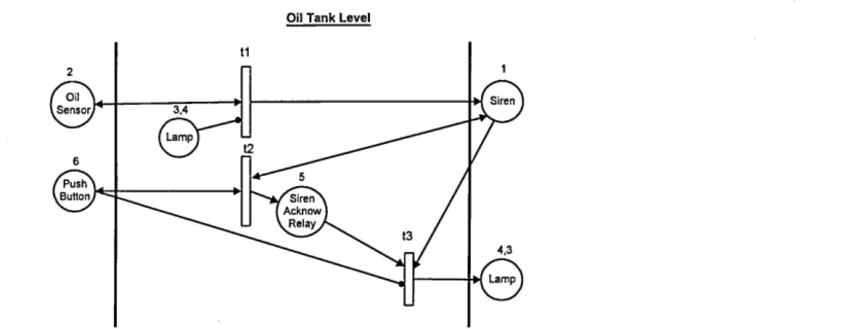
3.1.1 Design and Simulation

Gray’s methodology was applied to the control problem, Figure 3-1, and the PN graph

shown in Figure 3-2 was developed, directly from the requirements.

Oil T ank Level

Oil >

S en so rJ 3,4 W S iren

0 ^

P u sh

B utton ' S iren >

A cknow i R elay J

4,3

-M Lam p

Figure 3-2 PN Graph of Oil Tank Level Control Produced By Gray’s Methodology

As claimed, a readable design has been produced, in that the outputs are on the right-

hand side of the graph boundaries, the inputs are on the left-hand side of the

boundaries, and the internal logic is in between the boundary lines sequentially down

the page. However, it is not a dependable design, and Gray’s methodology does not

give full guidance to design dependable PLC control systems. For example, inhibitor

arcs had to be used but they are not part of his methodology. Instead, when

A methodology for developing resilient distributed control systems

A methodology for developing resilient distributed control

systems.

TAHOLAKIAN, Aram M.

Available from Sheffield Hallam University Research Archive (SHURA) at:

http://shura.shu.ac.uk/20418/

Sheffield Hallam University

uest

A Methodology for Developing

Resilient Distributed Control Systems

Aram Meguerditch Taholakian BEng

A thesis submitted in partial fulfilment of the

requirements of Sheffield Hallam University for the degree of

Doctor of Philosophy

Abstract

Table of Contents

List of Figures

Dedication

Acknowledgments

Declaration

Chapter 1

Introduction

Contents

1. Introduction

1.1 Automated Manufacture

Chapter 2

Background

Contents

2. Background

Chapter 3

The Application of Gray’s Methodology to an Overall DCS

3. The Application of Gray’s Methodology to an Overall DCS