Application of Ant Colony Optimization for the Solution of 3 Dimensional Cuboid Structures

http://dx.doi.org/10.4236/jcc.2014.24014

Application of Ant Colony Optimization for

the Solution of 3 Dimensional Cuboid

Structures

Hüseyin Eldem1, Erkan Ülker2

1_{Computer Technologies Department, Karamanoğlu Mehmetbey University, Karaman, Turkey} 2_{Computer Engineering Department, Selçuk University, Konya, Turkey}

Email: [email protected], [email protected]

Received November 2013

Abstract

Traveling Salesman Problem (TSP) is one of the most widely studied real world problems of find- ing the shortest (minimum cost) possible route that visits each node in a given set of nodes (cities) once and then returns to origin city. The optimization of cuboid areas has potential samples that can be adapted to real world. Cuboid surfaces of buildings, rooms, furniture etc. can be given as examples. Many optimization algorithms have been used in solution of optimization problems at present. Among them, meta-heuristic algorithms come first. In this study, ant colony optimization, one of meta-heuristic methods, is applied to solve Euclidian TSP consisting of nine different sized sets of nodes randomly placed on a cuboid surface. The performance of this method is shown in tests.

Keywords

Euclidean TSP; Ant Colony Optimization; Metaheuristic; Path-Relinking; Path Planning; Cuboid

1. Introduction

Traveling salesman problem (TSP) is a well-known problem in combinatorial optimization and it has been widely studied in the theoretical computer science and engineering applications. It is a problem that has to be solved by a salesman who travels between cities at minimum cost and return to the origin city. In this problem, one of the parameters including cost, time and path is optimized. The problem can also be stated as a Hamilto- nian cycle problem used in data modeling in computer sciences and investigated in the scope of a graph theory. Since 1950s, many researchers (e.g. computer scientists, mathematicians and others) have studied to develop methods that solve TSP finding the shortest route for cities in a given collection. If all costs between two cities are equal for both cities, TSP is named as symmetric, and otherwise, it is called asymmetric TSP.

TSP, which is evaluated in the area of discrete and combinatorial problems, has been widely studied in the area of similar popular problems. In the symmetric TSP, the distance between cities i and j is the same, i.e., dij=

dji. In the asymmetric TSP, this rule may not be valid all the time. Euclidean TSP is special cases of symmetric

TSP where the cities are positioned in Rm space for some m values for which the cost function satisfies the trian- gle equation. The ℓm norm, Euclidean norm if m = 2, is defined as ( 1| | )1/

d m m

i= xi yi

∑ − for m≥1 and (x1,···xm),

(y1,…ym)∈Rm. Two-dimensional Euclidean TSP is a popular and widely studied issue [1].

There are a great number of publications in literature devoted to TSP solution. Various heuristic algorithms, which give the possible closest solutions to the best ones in a certain time, based on simulated annealing [2], genetic algorithms (GA) [3-5], tabu search [6,7], artificial neural networks [8-10] and ant colony systems [11-16] have been developed. Meanwhile, local search algorithms like 2-opt and 3-opt were also used to solve TSP [17]. In order to attain better results, some researchers tried hybrid evolutionary algorithms [18-21]. Lately, 2-dimen- sional TSP problem has been transferred to the 3rd dimension and studied in literature. In [22-24], TSP applica- tions were performed for the points on 3D geometric shapes like sphere and cuboid. New algorithms were de- veloped through using genetic algorithms for TSP solution on cuboid geometric shape [22], Particle Swarm Op- timization (PSO) on cuboid shape [23] and genetic algorithms on 3D sphere shape [24].

Ant colony optimization (ACO), one of metaheuristic algorithms used to solve optimization problems, was proposed as a PhD thesis by Marco Dorigo in 1992 [15]. It is a probabilistic technique that is used to solve computational problems by investigating the probable ways on the graphs. It originates from the behavior of ants that find the shortest distance between their nests and the food source while seeking food and rapidly choose the shorter path. Various TSP applications were successfully solved by means of ACO techniques.

In the proposed study, TSP for points on a cuboid shape is solved by ACO algorithm. As 2-dimensional TSP

is a difficult problem and its reasons are given in the previous studies in literature, the fact that 3DTSP is a dif- ficult problem is not proved in this study. To the knowledge of the author, there is no study in literature that solves 3DTSP with ACO. In the existing TSP problems, coordinates or distances of points are known. The problem in this study differs from the existing TSP problems in that all points are located on a cuboid shape and the transition between points can be made through cuboid surface [22]. The developed 2D Euclidian TSP me- thods could be directly applied to 3DTSP with points in 3D space. However, TSP on a cuboid shape is different from 3DTSP as minimum distances between points on different surfaces cannot be calculated with Euclidian distance. As the travel takes places on the surfaces of cuboid, routes should be formed on the surfaces, as well, and not within the cuboid. The solutions could be used in route planning and collecting and placing pieces dur- ing the creation of a cuboid structure. This optimization method might be needed for small robot agents climb- ing up the wall, route planning, cleaning and painting. In this study, the performance of the developed method using ACO is tested, also its comparison with GA selected from the literature and advantages are presented. Pri- marily, the definitions of points on cuboid surface and determination of distances between points are explained. Subsequently, the adaptation of the problem to ACO is explained in the further parts of the paper.

2. Description of Cuboid Shapes

Cuboid is geometric shape which can be frequently seen in various products including wooden, metal, plastic and paper boxes, books, toys, dice, cupboards, furniture, rooms and buildings.

Cuboid is a three-dimensional object and a geometric shape with six rectangular faces (Figure 1). It has six faces, twelve sides and eight corners. Among geometric shapes, rectangular prism has a cuboid shape. Among three-dimensional objects, cube is a special form of cuboid, consisting of all square faces. As can be seen in

Figure 1, cuboid is one of the three-dimensional objects with height, width and length.

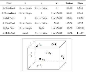
Cuboid objects have six faces: back (S0), bottom (S1), left (S2), front (S3), top (S4) and right (S5) (Figure 2).

Geometric information about a cuboid object located as back face z = 0, bottom y = 0 and left x = 0 is given in

Table 1. There are four sides and four corners for each face and some sides and corners are shared among the

rectangles forming the face (Table 1).

N points could be present on any of 6 cuboid faces. N = 7 cities (c0, c1,c2, c3,c4, c5, and c6) could be located on

cuboid faces (S3, S1, S5, S4, S4, S0, and S2) as in Figure 3.

The Euclidean distance of a pair of cities ci (xi, yi, zi) and cj (xj, yj, zj), is notated as dij (i,j= 1···n). Then the

distances between all pairs of cities can be computed in an N x N symmetric distance matrix D = [dij]. For a pair

Figure 1. A cuboid shape.

Figure 2. A cuboid object.

Table 1. Geometrical data of a cuboid.

Faces x y z Vertices Edges

S0 (Back Face) 0 < x < Length 0 < y < Height 0 0,1,3,2 0,2,3,1

S1 (Bottom Face) 0 < x < Length 0 0 < z < Width 0,4,5,1 0,8,4,9

S2 (Left Face) 0 0 < y < Height 0 < z < Width 0,2,6,4 1,10,5,8

S3 (Front Face) 0 < x < Length 0 < y < Height Width 4,5,7,6 4,6,7,5

S4 (Top Face) 0 < x < Length Height 0 < z < Width 2,3,7,6 3,11,7,10

S5 (Right Face) Length 0 < y < Height 0 < z < Width 1,3,7,5 2,11,6,9

two cities on adjacent faces. The pseudocode used for calculating the distance between ci and cj points is given

below:

if (face(ci) == face(cj))//SAME FACE

{

dij = Euclidean distance between the two points;

}

else if (face(ci) (opposite) face(cj))//OPPOSITE

{

calculate four alternative path distances di (through remaining faces)

dij = d0;

for(int k = 0; k < 4; ++k) if(dk < dij) dij = dk;

}

else if (face(ci) (adjacent) face(cj))//ADJACENT

{

d0 = calculate distance between the two points (through common edge of faces containing c1 and c2);

d1 = calculate distance between the two points (through the first common adjacent face of c1 and c2);

d2 = calculate distance between the two points (through the second common adjacent face of c1 and c2);

dij = min(d0, d1, d2);

}

The detailed information about pseudocode above used for calculating the distance between two points on cuboid faces is as follows:

a) If two cities are on the same face: Euclidean distance between two points is computed directly by

2 2 2

(x -x )_{j i} +(y -y )_{j i} +(z -z )_{j i} . The combinations are {S0, S0}, {S1, S1}, {S2, S2}, {S3, S3}, {S4, S4} and {S5, S5}

for any city pairs ci and cj.

b) If two cities are on the opposite faces: Thereare three alternatives in this case. 1) Front-Back {S3, S0}, 2)

Left-Right {S2, S5} and (3) Bottom-Top {S1, S4}. Four possible routes must be calculated for measuring the dis-

tance between opposite faces and the shortest path must be chosen. For instance, the possible routes for Left- Right case are:

I) Left-Front-Right II) Left-Back-Right III) Left-Top-Right IV) Left-Bottom-Right

In this case, the possible routes (d1, d2, d3 and d4) can be calculated, respectively, as follows:

for alternative (I)

y j i

d = y −y

(width ) length (width )

z j i

d = −z + + −z

2 2

1 y z

d = d +d

The routes can be similarly calculated for the other two cases mentioned above.

c) If two cities are on neighboring (adjacent) faces: Thereare again four alternative routes between adja-

cent faces in this case. However, if another face is visited for calculating the distance between adjacent faces, this alternative is neglected in calculations as it is the longest. For instance, for Front-Bottom neighboring faces, 1) Front-Bottom, 2) Front-Right-Bottom, 3) Front-Left-Bottom, and 4) Front-Top-Back-Bottom alternatives must be calculated. However, as the nonneighboring Top and Back faces are present for Front-Bottom transition in 4) Front-Top-Bottom alternative, it is not taken into consideration and neglected. In this case, the possible al- ternative routes (d1, d2 and d3) are calculated, respectively, as follows, and then, the shortest route is chosen.

for alternative (I)

x j i

(width )

z j i

d = −z +y

2 2

1 x z

d = d +d

There are 12 alternatives as neighboring faces: (Back-Bottom), (Back-Left), (Back-Top), (Back-Right), (Bot- tom-Left), (Bottom-Front), (Bottom-Right), (Left-Front), (Left-Top), (Front-Top), (Front-Right) and (Top- Right). The distance of each combination can be computed in a similar way by considering axis differences.

3. The Solution of

TSP

on a Cuboid Object by Using

ACO

3DTSP that would be applied to the surface of the cuboid is different from normal 2DTSP [22]. The salesman (ant or robot) could only travel between points located on the surface of the cuboid. The only difference in this problem is that the points are not located in the cuboid but on the surface of the cuboid.

The problem to be solved can be defined as the determination of the minimum tour distance for a salesman (ant) to travel all points (N points in total with known coordinates) located on a surface of a cuboid and come back to the original point, similar to standard TSP. In this study, it is aimed to solve the depicted problem by

ACO method.

After creating a distance matrix consisting of each pair of points, problem solution becomes the same as stan- dard TSP. After this stage, the solution of the problem can be examined by each method to solve TSP, which is depicted in the literature survey of the introduction part. In this paper, solutions were obtained for specific num- ber of set of points by using ACO.

General structure of the ACO:

initializealledgesto (small) initialpheromonelevelτ0;

placeeachantonarandomlychosencity;

foreachiterationdo:

dowhileeachanthasnotcompleteditstour:

foreachantdo:

moveanttonextcitybytheprobabilityfunction androulettewheelselection

end;

end;

foreachantwithacompletetourdo:

evaporatepheromones;

applypheromoneupdate;

if (antk’stourisshorterthantheglobalsolution) updateglobalsolutiontoantk’stour end

end

Based on this general structure, initial values of ACO algorithm are set. Accordingly, initial pheromone loads of each side are updated and stored in pheromone matrix. Using the notations in Title 2, distance matrix consist- ing of distances between each point and every other point is created. In ACO algorithm, each ant giving solution,

i.e., agent ant is located random cities initially. In each iteration, the following Equation (1) is used to select the next city to be visited by ants.

( )

( )

( )

[ ]

if j allowed . . ij ij k ij k ik ik t p t t β α α β τ η τ η   _{ }         =_ ∈    _{ } 

∑

where, τij

( )

1/dij. dij, is the distance between two points on a cuboid. α and β are two parameters which control the impor-

the best results when the iterations are complete.

4. Experimental Results

Analyses were performed in a computer of Intel Core 2 Duo P8700 2.53 GHz processor and 4 GB RAM. In coding phase of the method, Matlab R2010a programming language was used and called cuboidTSP software. The simulation results obtained through this software were produced for the points N = 10, 50, 100, 250 on a 1000 × 1000 × 1000 cuboid.

Simulations were repeated 100-times for each value of N. A new random point set was generated for each trial. In this study, this approach was preferred instead of the method given in [22], i.e., utilization of the predefined set of points to generalize the results on the cuboid. The performance of the suggested method was compared to the results reported by [22].

In [22], Aybars reported results for five different GA generation sizes (20, 40, 60, 80, 100) and the points of N = 10, 50, 100, and 250 for TSP application on cuboid through GA. For each generation, Aybars fixed the size of the population as 250. While the mutations of individuals in a population observed in each generation can be defined as evolution, the total evolution is equal to multiplication of the size of the population by the number of generation. In the literature, for the solution of TSP, it is convenient to take the number of ants to the number of cities. For this reason, in the proposed study, the number of ant was taken equal to the number of points in the cuboidTSP. In order to make a comparison with a GA publication taken from the literature and to have an equal number of evolutions for ACO with that depicted in the [22] for each generation, the number of tour is determined by using the following equation:

Generation Size Population Size

Number of Tours .

Number of Ants

GA GA

ACO

ACO ×

= (2)

The results representing the optimum length of the tour were obtained for different number of evolutions, i.e., 20, 40, 60, 80 and 100 evolutions. For all experiments, the number of ants were equal to that of points and α = 1,

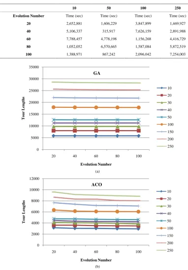
β = 5 and ρ = 0.50 (the coefficient of evaporation) were kept constant. The calculated average tour distances both for GA and for the proposed ACO approach are given in Table 2. Meanwhile, mean calculation durations advised for ACO in this paper are shown in Table 3. The width, height and length of the cuboid were all taken as 1000. A cuboid of 1000 × 1000 × 1000 size is preferred for the sake of understandability and easy assessment of the results.

When the results of GA and those of ACO were compared, see in Table 2, it was observed that the results of

ACO algorithm were much more successful than GA for cuboidTSP. For instance, when evolution number for 150 points is taken as 100, the tour length obtained with GA could be shortened by 1/3. This rate is even higher for 200 and 250 points. It can be seen in Figure 4 that tour lengths are within [5000, 30,000] for GA and [2000,

10,000] for ACO.

Through increasing the numbers of tour and evolution in algorithm, the optimum results can be further im- proved, as can be seen in Table 2 and Figure 4. ACO parameters are kept constant in the study. By altering the

ACO parameters, better results can be obtained. Apart from ACO, the results can also be improved through using available hybrid methods for TSP solution.

Table 2. Calculated average cuboidTSP tour lengths with GA [22] and ACO for N = 10, 50, 100, 250 points on the surface of the cuboid.

Evaluation number

10 50 100

GA ACO GA ACO GA ACO GA ACO

20 5805 3138 12,631 4755 17,938 6340 28,612 9588

40 5805 3027 12,614 4731 17,894 6135 28,430 9138

60 5805 3016 12,609 4653 17,874 6083 28,347 9011

80 5805 2971 12,602 4614 17,853 6055 28,293 8906

Table 3. Calculated average cuboidTSP tour computation times with ACO for N = 10, 50, 100, 250 points on the surface of the cuboid.

10 50 100 250

Evolution Number Time (sec) Time (sec) Time (sec) Time (sec)

20 2,652,881 1,606,229 3,847,899 1,469,927

40 5,106,337 315,917 7,626,159 2,891,988

60 7,788,457 4,778,198 1,156,268 4,416,729

80 1,052,052 6,570,665 1,587,084 5,872,519

100 1,388,971 867,242 2,096,042 7,254,003

(a)

(b)

Figure 4. Average tour lengths for different amount points on the surface of the cuboid founded by GA [22] and ACO solutions.

5. Conclusion

The main contribution of this paper is to show the applicability of TSP solutions cuboid objects and structures of

0 5000 10000 15000 20000 25000 30000 35000

20 40 60 80 100

T

o

ur

L

eng

ths

Evolution Number

GA

10

20

30

40

50

100

150

200

250

0 2000 4000 6000 8000 10000 12000

20 40 60 80 100

T

o

ur

L

e

ng

ths

Evolution Number

ACO

10

20

30

40

50

100

150

200

any size. The aim of the study is to develop a simple yet effective method through testing ACO method frequently used in TSP problems to determine optimum route by visiting all points on cuboid. For this purpose, TSP opti- mization results for different-sized point sets were obtained in the first place through ACO method for points on a cuboid object.

It is quite important for saving from time in route planning of air vehicles like helicopter in search and rescue operations on cuboid structures during natural disasters like fire or earthquake. Furthermore, the successful op- timization of the method could be used in maintenance (painting etc.) or cleaning operations on cuboid structures. This method can be used in any kind of applications requiring the use of programmable wall climbing robots. It is possible that 3D applications of TSP problems will become more important with the advancement of robotic in- dustry in the future.

The current optimization techniques in literature have been generally developed in 2D environments. Devel- oping and using these techniques in 3D environments will definitely inspire the development of optimization techniques in different fields. And it is observed that 3D techniques are gradually started to be developed.

ACO, which can be effectively used in the solution of current 2DTSP by giving optimum results, was also successful for cuboidTSP. When the results of TSP application on cuboid proposed by Aybars in [22] using GA

and the results of the method proposed in the current study are compared, it is seen that ACO provides more successful results in cuboid TSP than GA.

In the future studies, other methods in the solution of TSP, e.g. PSO, can be tested for the solution of the cu- boidTSP. Meanwhile, cuboidTSP problems can be studied by hybrid utilization of ACO and PSO methods.

References

[1] Arora, S. (1996) Polynomial Time Approximation Schemes for Euclidean TSP and Other Geometric Problems. Pro- ceedings of the 37th Annual IEEE Symposium on Foundations of Computer Science, Burlington, 14-16 October 1996, 2-11.

[2] Kirkpatrick, S., Gelatt, C.D. and Vecchi M.P. (1983) Optimization by Simulated Annealing. Science, 220, 671-680. http://dx.doi.org/10.1126/science.220.4598.671

[3] Tsujimura, Y. and Gen, M. (1998) Entropy-Based Genetic Algorithm for Solving TSP. Knowledge-Based Intelligent Electronic Systems, Adelaide, 285-290.

[4] Goldberg, D.E. (1989) Genetic Algorithms in Search, Optimization, and Machine Learning. Addison-Wesley, Reading.

[5] Holland, J.H. (1975) Adaptation in Natural and Artificial Systems. University of Michigan Press, Ann Arbor.

[6] Glover, F. (1989) Tabu Search—Part I. ORSAJournalonComputing, 1, 190-206. http://dx.doi.org/10.1287/ijoc.1.3.190

[7] Glover, F. (1990) Tabu Search—Part II. ORSAJournalonComputing, 2, 4-32. http://dx.doi.org/10.1287/ijoc.1.3.190 [8] Hopfield, J.J. and Tank, D.W. (1985) Neural Computation of Decisions in Optimization Problems. BiologicalCyber-

netics, 52, 141-152.

[9] Kohonen, T. (1995) Self-Organizing Maps. Springer, Berlin. http://dx.doi.org/10.1007/978-3-642-97610-0

[10] Shinozawa, K., Uchiyama, T. and Shimohara, K. (1991) An Approach for Solving Dynamic TSPs Using Neural Net- works. ProceedingsoftheIEEEInternationalJointConferenceonNeuralNetworks, 3, 2450-2454.

[11] Colorni, A., Dorigo, M. and Maniezzo, V. (1991) Distributed Optimization by Ant Colonies. In: Varela, F. and Bour-gine, P., Eds., ProceedingsoftheEuropeanConferenceonArtificialLife, ECAL’91, Paris, Elsevier Publishing, Ams- terdam, 134-142.

[12] Colorni, A., Dorigo, M. and Maniezzo, V. (1992) An Investigation of Some Properties of an Ant Algorithm. In: Maenner, R. and Manderick, B., Eds., ProceedingsoftheSecondConferenceonParallelProblemSolvingfromNa- ture, Brussels, PPSN II, North-Holland, Amsterdam, 509- 520.

[13] Dorigo, M. (1992) Optimization, Learning and Natural Algorithms. Ph.D. Thesis, Politecnico di Milano, Italy.

[14] Gambardella, L.M. and Dorigo, M. (1996) Solving Symmetric and Asymmetric TSPs by Ant Colonies. Proceedingsof theInternationalConferenceonEvolutionaryComputation, Nagoya, 20-22 May 1996, 622-627.

[15] Dorigo, M. and Gambardella, L.M. (1997) Ant Colony System: A Cooperative Learning Approach to the Traveling Salesman Problem. IEEE Transactıons on Evolutıonary Computatıon, 53-66.

[17] Johnson, D.S. and McGeoch, L.A. (1997) The Traveling Salesman Problem: A Case Study in Local Optimization. In: Aarts, E.H.L. and Lenstra, J.K., Eds., LocalSearchinCombinatorialOptimization, John Wiley & Sons, New York, 215-310.

[18] Lee, Z.J. (2004) A Hybrid Algorithm Applied to Travelling Salesman Problem. Networking, SensingandControl, Pro- ceedingsoftheIEEEInternationalConference, 237-242.

[19] White, C.M. and Yen, G.G. (2004) A Hybrid Evolutionary Algorithm for Traveling Salesman Problem. Congresson EvolutionaryComputation (CEC2004), 1473-1478.

[20] Marinakis, Y., Migdalas, A. and Pardalos, P.M. (2005) A Hybrid Genetic-GRASP Algorithm Using Lagrangean Re- laxation for the Traveling Salesman Problem. JournalofCombinatorialOptimization, 10, 311-326.

http://dx.doi.org/10.1007/s10878-005-4921-7

[21] Tsai, C., Tsai, C. and Tseng, C. (2004) A New Hybrid Heuristic Approach for Solving Large Traveling Salesman Problem. InformationSciences, 166, 67-81. http://dx.doi.org/10.1016/j.ins.2003.11.008

[22] Uğur, A. (2008) Path Planning on a Cuboid Using Genetic Algorithms. InformationSciences, 178, 3275-3287. http://dx.doi.org/10.1016/j.ins.2008.04.005

[23] Su, S.B. and Cao, X.B. (2013) Jumping PSO with Expanding Neighborhood Search for TSP on a Cuboid. Chinese JournalofElectronics, 22, 202-208.