Forecasting Vix
Degiannakis, Stavros
Department of Statistics, Athens University of Economics and
Business
2008
Online at
https://mpra.ub.uni-muenchen.de/96307/
F o r e c a s t i n g V I X
Dr. Stavros A. Degiannakis
Department of Statistics, Athens University of Economics and Business1
A b s t r a c t
Implied volatility index of the S&P500 is considered as a dependent variable in a
fractionally integrated ARMA model, whereas volatility measures based on interday and intraday datasets are considered as explanatory variables. The next trading day’s implied volatility forecasts provide positive average daily profits. All the forecasting
information is provided by the VIX index itself. There is no incremental predictability
from both realized volatility computed from intraday data and conditional volatility
extracted from an Arch model. Hence, neither the interday volatility nor the use of
intraday data yield any added value in forecasting the S&P500 implied volatility index.
However, an agent cannot utilize VIX predictions in creating abnormal returns in
implied volatility futures market.
Keywords: ARCH, ARFIMAX, Fractional Integration, Volatility Forecasting, VIX
Index.
JEL: C32, C52, C53, G15.
1 I n t r o d u c t i o n
Financial literature is full of evidence that short-term volatility is predictable. Since
Engle (1982) introduced the autoregressive conditional heteroskedasticity (Arch) model,
numerous methods have been proposed for predicting future volatility of assets returns.
Presently, in a forecast-based evaluation framework, extended versions of Arch
volatility specifications have been applied providing added predictive ability in various
1Department of Statistics, Athens University of Economics and Business 76, Patision street, Athens GR-104 34,
areas such as option pricing, risk management, portfolio analysis, etc. In the past years, based on Andersen and Bollerslev’s (1998) seminal paper, the use of intraday datasets has rekindled the interest of academics to forecast variability of asset returns. The
realized volatility, which is defined as the sum of the squared intraday returns, is mainly
modeled by autoregressive fractionally integrated moving average with exogenous
variables (ARFIMAX) models.
On the other hand, implied volatility2, first noted by Latane and Rendleman (1976),
is considered by many studies as an accurate predictor of future volatility. However, as
very well documented by Blair et al. (2001), a number of studies characterize implied
volatility measures as less informative than volatility estimated from asset returns,
because they induce important biases and contain mis-specification problems. In the
recent past, the implied volatility index (VIX) of the Chicago Board of Options
Exchange (CBOE) eliminated such measurement errors. As a result, market participants
consider the VIX index as the world’s premier barometer of investor sentiment and
market volatility.
Blair et al. (2001) estimated an Arch model with Glosten’s et al. (1993) conditional variance specification. They considered the VIX index of S&P100 and the realized
volatility based on five-minute S&P100 returns as explanatory variables. They
concluded that the implied volatility index provides more accurate forecasts than either
the interday volatility extracted from daily return series or the intraday realized
volatility. Koopman et al. (2005) compared the forecasts of various classes of volatility
models with realized volatility. They confirmed that volatility forecasts extracted from
models of daily returns (such as Arch and Stochastic Volatility models) are less accurate
than forecasts based on VIX index. However, models based on realized volatility (such
as ARFIMAX and Unobserved Components ARMA models) outperform models with
implied volatility.
The aforementioned studies consider the implied volatility index as an explanatory
variable in forecasting either the interday conditional volatility or the intraday realized
2 Implied volatility is the standard deviation of the return on the asset, which would have to be inputted
into a theoretical option pricing formula to yield a theoretical value identical to the price of the option in
volatility. The present study is the first that models an implied volatility index as a
dependent variable. The main purpose of the study is to investigate whether the use of
intraday datasets or conditional volatility extracted from an Arch model provides any incremental predictive ability in forecasting the next day’s implied volatility. We present evidence that all the forecasting information is provided by the implied volatility
index. Neither interday nor intraday volatility measures supply any statistically
significant incremental information. The results of the paper point to a fairly important
conclusion, that the VIX index is hard to forecast and does not seem to be very closely
connected to the volatility of the underlying index. The VIX index is supposed to
measure the market's volatility forecast over the future, thus it seems to have little
connection to observable behavior of the actual S&P500 volatility. Finally, we conclude
that in the case of trading VIX futures instead of VIX itself, there is no economic gain
from forecasting the VIX index.
The structure of the paper is as follows. The second section presents the dataset,
while the third one describes the estimation procedure of volatility forecasts. The
proposed method to evaluate the forecasting performance is presented in section four,
whereas section five explores the forecasting ability of the models under investigation.
Section six investigates whether an agent can utilize volatility index forecasts to create
abnormal returns in the implied volatility futures market. Section seven concludes the
paper and provides some ideas for further research.
2 I n t r a d a y a n d I n t e r d a y D a t a s e t s
The S&P500 and VIX indices were obtained from the CBOE for the period 3rd
January, 1990 to 24thDecember, 2003. Index VIX measures the market’s expectation of
30-day volatility implicit in the prices of near-term S&P500 options. The result forms a
composite hypothetical option that is at-the-money and has 30 calendar (22 trading)
days to expiration. Index VIX represents the implied volatility for this hypothetical
option. On September 22, 2003, the CBOE announced a new computation of its
volatility index. The old VIX changed to VXO. The new VIX is based on S&P500
index options in its calculation, as opposed to just eight options of VXO3. In the present
study as VIXclose the new VIX index is considered.
The intraday dataset was obtained from Olsen and Associates for the period
ranging from 2nd January, 1997 to 24th December, 2003. The realized volatility on day t
is computed as:
1 1 2 , , 1 2 2 2 ln ln 100 ˆ ˆ ˆ m j t m j t m j oc co oct P P
RV
, (1)
where P m,t are the S&P500 prices on day t with m observations per day,
T t t m toc T P P
1 2 , 1 , 1 1 2 ln ln ˆ
is the open-to-close sample variance, and
T t t t mco T P P
1 2 1 , 1 , 1 1 2 ln ln ˆ
is the close-to-open sample variance. Five-minute
linearly interpolated prices, from 08:30 CST until 15:00 CST, or m79, are considered
for avoiding market microstructure frictions without lessening the accuracy of the
continuous record asymptotics. The scaling factor ˆ 2
ˆ2 ˆ2
oc oc co
accounts for the
overnight returns without inserting the noisy effect of daily returns4.
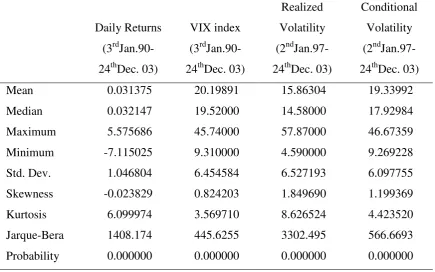
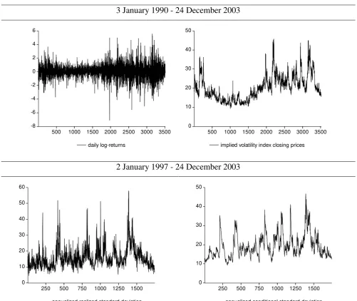
Table 1 presents the descriptive statistics of daily log-returns
100ln
P 1,t P 1,t1
,implied volatility index closing prices (VIXclose), annualized realized standard deviation
252RV
, and annualized conditional standard deviation 252 , extracted from TARCH model in Equation (3), whereas Figure 1 depicts the relative line graphs. Figure
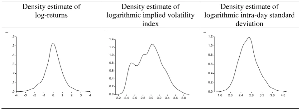
2 plots the distributions of daily log-returns, logarithmic implied volatility index, and
logarithmic intraday standard deviation. The density estimates are based on the normal
Kernel with bandwidths method calculated according to Equation 3.31 of Silverman
(1986). The daily log-returns indicate nonzero skewness and excess kurtosis relative to
that of the normal distribution. The annualized unconditional volatility of daily
log-returns is 16.62%, (1.0468* 252 ). The mean value of the implied volatility index is
3 For details about the construction of CBOE volatility indices refer to Whaley (1993), Fleming et al.
(1995), as well as to CBOE VIX whitepaper in http://www.cboe.com/micro/vix/vixwhite.pdf.
4 The method we follow to account for the effects of overnight returns and intraday noise is similar to
20.19%. The average annualized realized volatility is 15.86%, whereas during the same
period the annualized unconditional (conditional) volatility of daily returns is 20.55%
(19.34%). The intraday volatility is much less as in Blair et al. (2001), who noted that
this is a consequence of positive correlation between consecutive intraday returns. The
intraday standard deviation is leptokurtic and skewed to the right. Our findings are in
line with the previous studies (i.e., Ebens 1999, Andersen et al. 2001, Thomakos and
Wang 2003, Giot and Laurent 2004) as the intraday logarithmic standard deviation is
close to the normal distribution but statistically distinguishable from it. The Jarque-Bera
(56.40), Anderson-Darling (3.94), and Crámer-Von Misses (0.63) statistics reject the
hypothesis of normality at any level of significance.
3 V o l a t i l i t y M o d e l s
The logarithm of the VIX index is regarded as the dependent variable in an
ARFIMAX specification with normally distributed innovations. The interday
conditional volatility and the intraday realized volatility are considered as exogenous variables to investigate their contribution in forecasting the next day’s VIX value. The ARFIMAX model is defined as:
t t
t
t
td u bL f RV f y w w VIX L
aL
1 ln 1
1 0 1 1 1 1 2 1 (2)
2 . . . , 0 ~ u d i i t Nu ,
where ,
252
1
closet t VIX
VIX , yt 100ln
P 1,t P 1,t1
is the return series from day 1
t to t, P t1 is the S&P500 closing price at day t, and L is the lag operator. The AFRIMAX model was introduced by Granger (1980) and Granger and Joyeux (1980)
and was applied first in modeling realized volatility by Ebens (1999). The fractional
integration parameter, d, captures the slow hyperbolic decay of the response of the
implied volatility index to past shocks, whereas the parameter w1 takes into account the
response of daily S&P500 returns to the implied volatility index. The realized volatility
specification is modeled in the forms
2
1 2
1 1
1 , ,ln
t t t
t RV RV RV
RV
f . The conditional
volatility extracted from an Arch model is considered either as the in-sample volatility
estimated at day t1 given the information set that is available at the same day,
t1|t1
f , or as the out-of-sample volatility of day t given the information set that is
available at day t1, f
t|t1 . Thus,
2 1 | 2 1 | 1 | 2 1 | 1 2 1 | 1 1 | 1
1 , ,ln , , ,ln
t t t t t t tt tt tt
t
The parameters 1 and 2 represent the added contribution of realized intraday
volatility and conditional interday volatility, respectively. Since
2, 0
~ u
t N
u , the
one-day-ahead VIX is
2
| 1 *
|
1t exp ln t t 0.5 u
t VIX
VIX .
In the sequel, we propose an Arch model for computing the conditional volatility
on the S&P500 index daily returns. The TARCH model, which was introduced by
Glosten et al. (1993), with skewed Student t distributed standardized innovations,
represents a parsimonious Arch model that accounts for the asymmetric response of
innovations to volatility:
, , ; 1 , 0 ~ 1 2 1 2 1 1 1 2 1 1 0 2 . . . 1 1 0 t t t t t t t d i i t t t t t t b z d z a a g v skT z z L c c y (3)where
2 1 1 2 1 2 2 2 2 1 , ; v d t t t g v m sz g g s v v v g v z skT , g is the
asymmetry parameter, v2 denotes the degrees of freedom of the distribution,
. isthe gamma function, dt 1 if zt 0 and dt0 otherwise,
1
1
2 2
2
1
v v v g g
m and 2 2 2 1
m g g
s . The
autoregressive component of the conditional mean is considered to account for the
nonsynchronous trading effect. The in-sample conditional variance is estimated as
2 | 1 2 | 1 1 0 2| t t
t t t t t t t t
t a a d b
. The one-day-ahead conditional variance
forecast is computed as
2|2 | 0
2 |
1 tt
t t t t t t t t
t a a d b
.
4 E v a l u a t i o n M e t h o d o l o g y
The common method to evaluate the forecasting performance is through defining a
statistical loss function that measures the distance between predictions and observations.
In our study, we create an economic loss function that calculates the cumulative returns
from trading VIX index on a daily basis. If the VIX price forecast is greater than the
VIX closing price, the VIX index is bought. If the VIX price forecast is less than the
VIX closing price, the index is sold. For each transaction, traders should pay a
transaction cost. Moreover, trades will be executed only when profits are expected to
when the difference between forecast and observed VIX prices exceeds the amount of
filter F . The model’s i average daily return after a transaction cost, X, is
i nt closet s
t closet
i t t close t close i VIX X VIX d VIX VIX s R 1 , 1 , , 1 , 1 * *
, (4)
where s* is the number of trading days, i
n is the number of transactions, i 1
t
d if
F VIX
VIXt*1i|t t , i 1
t
d if VIXt* 1i|t VIXtF and i 0
t
d otherwise5.
Besides the average daily return, the Sharpe ratio is computed as the ratio of the
annualized average returns with annualized standard deviation of daily returns:
i iR V R
SR 252 . (5)
To investigate whether the model achieves the highest performance and is
significantly different from its competitors, we apply the Diebold and Mariano (1995)
test. The null hypothesis of equivalent predictive ability of models i and i against the
alternative hypothesis that the benchmark model i is superior to model i is tested. Let
close, 1 close,
close,
i
t t t t
i t
t
VIX VIX d Xn
r
VIX
denote the return on day t based on model i,
where nt 2 if
1
1
i
t i t d
d , nt 0 if
i t i t d
d 1, nt 1 otherwise. For
i t i t i it r r
z ,
-, the Diebold–Mariano (DM) statistic is the t-statistic derived by the
regression of ii t
z , on a constant with HAC standard errors.
5 E m p i r i c a l R e s u l t s
The models were estimated in the G@RCH and ARFIMA packages of Ox. The first
VIX forecast is generated for January 2nd, 2002. For each trading day, the models are
re-estimated based on the rolling sample of constant size equal to s1249 trading days,
hence, *
s 499 one-day-ahead volatility forecasts are estimated. We take into
consideration a transaction cost of $0.2, which reflects 20 times the minimum price
5 Two transactions costs are charged because we have to unwind yesterday's position and put a new one
on today. Both transaction costs are applied to today’s returns. Yesterday's transactions cost could be
interval of VIX point, and consider various values for the filter and, in particular,
0.10.40
F .6
The orders of the autoregressive and the moving average components of the
ARFIMAX framework are not determined based on in-sample model selection criteria,
such the Akaike’sand Schwarz’s information criteria, as a good in-sample performance
of a model is not a prerequisite for its good out-of-sample precision7. We have
estimated various versions of the framework given by Equation (2), that is, higher
orders of the autoregressive and the moving average components, and different sets of
exogenous variables, but we exhibit the models that are useful for the presentation of
the results8. The ARIMAX model for zero autoregressive order and moving average
order of one achieves the highest forecasting performance.
In the sequel, we name the model ARFIMAX, but the autoregressive component is
omitted. The specification given by Equation (2) is estimated for 1 2 0 as well as
for the various functional forms of the realized intraday and the conditional interday
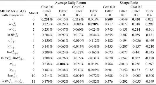
volatility, providing 12 models in total. Table 2 presents the 12 models, numbered from
0 to 11. For example, model 1 denotes the ARFIMAX model in Equation (2) with the
2 1
t
RV as exogenous variable. According to Table 2, which presents the average daily
returns and the Sharpe ratios of these models, the daily returns, without assuming any
trading cost, are between 0.141% and 0.251% with Sharpe ratios ranging from 0.453 to
0.809. The ARFIMAX model, without any functional form of RVt1 or t1 as the
exogenous variable, achieves the highest profit. However, after a transaction cost of
$0.2, the average returns are negative in all the cases. We proceed on a trade only when
profits are predicted to exceed the assumed trading cost. Hence, trades are executed only when the absolute difference between forecast and today’s VIX price exceeds the
amount of the filter F. For $0.2 trading cost and filter, the ARFIMAX model that takes
into consideration volatility information solely from the lag values of the VIX index is
still the model with the highest returns. After a trading cost of $0.2 and a filter rule of
6 Fa
bc denotesc ,
b c b a b a a
T , , 2 ,..., .
7 For more details see Brooks and Burke (2003), Angelidis et al. (2004), and Degiannakis and Xekalaki
(2007).
$0.4, the ARFIMAX model with the realized variance RVt21 as the exogenous variable
is the best performing model. In general, all the forecasting information is provided by
the VIX index. There is no substantial improvement in the forecasting ability of the
models that take into consideration information from interday or intraday S&P500
volatility. Models 1 (with RVt21 as exogenous variable) and 8 (with 2
1 |t t
as exogenous
variable) as well as the model without any exogenous volatility information achieve the
highest rate of returns.
Table 3 presents the percentage of long and short trading positions for trading VIX
index based on the signals generated by the predictions of the models. Without
transaction costs, the long and short trading positions are suggested, on average, in 65%
and 35% of the trading days, respectively. In the cases of a $0.2 and $0.4 filters, the
long positions are also more often suggested than the short ones. The average daily
profit from always taking long trading positions is 0.06% without assuming any trading
cost and negative in the case of adding a trading cost and any filter.
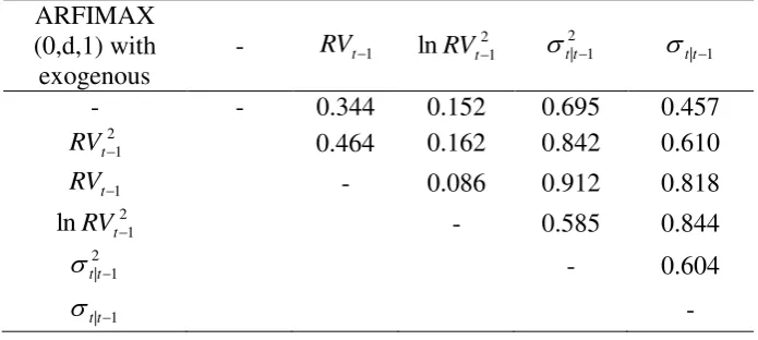
Table 4 presents the corresponding p-values of the DM test for the null hypothesis
that model i has statistically equal loss function as model i. The null hypothesis is not rejected at any rational level of significance, indicating that realized volatility and the
extracted volatility from the Arch model do not provide any significant incremental
predictive ability in forecasting VIX index. The model without any functional form of
1
t
RV or t1 as exogenous variable has statistically equal loss function as its competing
models9.
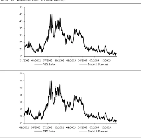
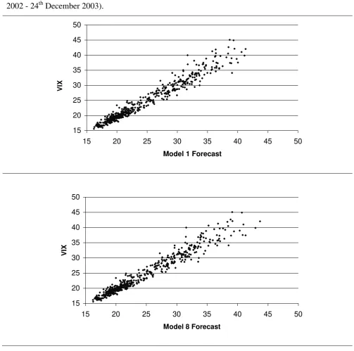
Figure 3 depicts, indicatively, the cumulative daily returns of Models 1 and 8.
Figure 4 plots the VIX index and the corresponding one-day-ahead forecasts of Models
1 and 8, whereas Figure 5 presents the scatter plot of VIX index and the one-day-ahead
VIX forecasts. In both cases, the one-day-ahead prediction line graphs are almost
9 The evaluation was also conducted based on statistical loss functions that measure the distance between
predicted and actual VIX values. The minimum values of MSE and MAE criteria were achieved by
Model 5. The hypothesis that Model 5 has superior predictive ability is not rejected at any reasonable
level of significance. Therefore, if the evaluation were based on the distance between observed and
predicted values, we would have concluded that the conditional volatility extracted from the TARCH
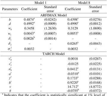
indistinguishable from the index itself. Table 5 presents the estimated parameters of the
Models 1 and 8 by using the entire dataset. All the parameters except the constant
coefficients are statistically significant at least at 5% level of significance. The variance
is characterized by slowly mean-reverting fractionally integrated process as the degree
of integration is lower than 0.5 (although statistically equal to 0.5 for the intraday
model) and therefore, there are indications that the intraday volatility is covariance
stationary. Cases in which the logarithmic realized volatility of stock indices is the
dependent variable, parameter d was estimated at 0.46 and 0.48 for the CAC40 and S&P500 indices, respectively, by Giot and Laurent (2004), less than 0.4 (Dow Jones
Industrial Average) by Ebens (1999), and around 0.45 (S&P500) by Thomakos and
Wang (2003). In regard to the TARCH model, the asymmetry between past bad or good
news and volatility is statistically significant and the estimated parameters of the
skewed Student-t distribution indicate that the innovations are asymmetric and
leptokurtic.
6 T r a d i n g G a m e w i t h V I X F u t u r e s
VIX index is a volatility forecast, not an asset. Hence, in reality, we cannot create a
position by buying or short-selling the index itself. On March 26th, 2004, the CBOE
announced the trading of futures on the VIX index. VIX futures are contracts on
forward 30-day implied volatilities. They are quoted 10 times the value of VIX and the
contract multiplier is $100. The minimum price interval is 0.01 of VIX point or $10 per
contract. The final settlement date is the Wednesday prior to the third Friday of the
expiring month.
The data of futures on VIX were obtained from the CBOE over the sample period
of 26th March, 2004 through 23rd February, 200610. We repeat the estimation of the
model framework given in Equation (2) by expanding the sample period up to 23rd
February, 2006. The loss function given in Equation (4) is measured by replacing
close,t
VIX with one tenth of the VIX futures settlement value. The futures with contract
months on the February quarterly cycle and a maturity period of length no shorter than 4
trading days were considered as these are the contracts with the highest trading volume.
In the case of trading VIX futures instead of VIX itself, there is no economic gain from
forecasting the VIX index. Thus, an agent who applies the proposed forecasting model
is unable to create trading strategies that yield abnormal returns. Of course, we can
reasonably conclude that the VIX index on day t expresses the volatility expected for
the period from day t to day t30, while the next month’s VIX futures express the volatility expected for the period from the expiration day to 30 days ahead.
The VIX itself, an approximation to the overall implied volatility of the S&P500
options, is a prediction of future volatility. VIX futures on the other hand is a prediction
of where the prediction of future volatility will be on the day that the future expires. The
futures contract is based on a future version of the VIX index. According to Figure 6,
which presents the VIX and VIX futures scatter plot, the correlation between VIX and
VIX futures is not high and can be even negative. For example, in 26% of the trading
days the VIX and VIX futures log-returns have opposite signs.
7 C o n c l u s i o n s
We provided an empirical model that produced adequate one-day-ahead predictions
of VIX index. Instead of evaluating forecasts based on statistical loss functions, we
measured an economic loss function as the average return from trading VIX index on a
daily basis. All the forecasting information is provided by the VIX index itself. Both
realized volatility and conditional volatility extracted from an Arch model were
considered as exogenous variables in the model, but they did not provide any
incremental information in forecasting VIX index. Hence, there is no added value either
from the use of the more hard-to-collect intraday datasets or from estimating an Arch
model using daily datasets.
Blair et al. (2001) and Koopman et al. (2005) also provided evidence that interday
volatility does not provide more accurate forecasts than the implied volatility. We also confirmed Blair’s et al. (2001) finding that the intraday volatility measure does not yield significant incremental forecasting information.
An interesting point that is left for further study is the evaluation of the models’ predictability in a multiperiod framework. Moreover, there is not yet a standard method
of computing realized volatility based on the intraday datasets. Recently, Zhang et al.
(2003), Engle and Sun (2005), and Hansen and Lunde (2005) proposed various
realized variance is still an open area for research. Whether the new methods of
computing realized volatility will increase its forecasting ability is also a very
interesting topic.
An important issue that is still unanswered and a future study should be focused on
is whether the VIX index is efficient or not. The dynamics of the VIX, which is
supposed to measure the market's volatility forecast over the next 30 days, seem to have
little connection to observable behavior of the actual S&P500 volatility. This could
mean that the VIX is highly efficient and fully discounts the information that can be
extracted from recent historical data, or it could mean that the VIX itself is inefficient
and valuable information from Arch type models (or realized volatility measure) is
ignored?
In the previous section we discovered that forecasts of the VIX index are unable to
provide any information in forecasting VIX futures. VIX futures were introduced on
March 26th, 2004. Hence, adequate sample size is not available to estimate the proposed
model with the VIX futures series as dependent variable. When an adequate sample size
of VIX futures becomes available, it will be interesting to investigate whether an
ARFIMAX model on the VIX futures can produce forecasts that yield positive profits.
A c k n o w l e d g e m e n t
I would like to thank Pierre Giot and Sébastien Laurent for the availability of their program codes and Stephen Figlewski for his valuable and constructive suggestions.
R e f e r e n c e s
1. Andersen, T. and Bollerslev, T. (1998). "Answering the Skeptics: Yes, Standard
Volatility Models Do Provide Accurate Forecasts." International Economic
Review, 39, 885-905.
2. Andersen, T., Bollerslev, T., Diebold, F.X. and Ebens, H. (2001). "The
Distribution of Realized Stock Return Volatility." Journal of Financial
Economics, 61, 43-76.
3. Angelidis, T., Benos, A. and Degiannakis, S. (2004). "The Use of GARCH
Models in VaR Estimation." Statistical Methodology, 1(2), 105-128.
4. Blair, B.J., Poon, S-H and Taylor S.J. (2001). "Forecasting S&P100 Volatility:
High-Frequency Index Returns." Journal of Econometrics, 105, 5-26.
5. Brooks, C. and Burke, S.P. (2003). "Information Criteria for GARCH Model
Selection." European Journal of Finance, 9, 557-580.
6. Degiannakis, S. and Xekalaki, E. (2007). "Assessing the Performance of a
Prediction Error Criterion Model Selection Algorithm in the Context of ARCH
Models." Applied Financial Economics, 17, 149-171.
7. Diebold, F.X. and Mariano, R. (1995). "Comparing Predictive Accuracy."
Journal of Business and Economic Statistics, 13(3), 253-263.
8. Ebens, H. (1999). "Realized Stock Volatility." Department of Economics, Johns
Hopkins University, Working Paper, 420.
9. Engle, R.F. (1982). "Autoregressive Conditional Heteroskedasticity with
Estimates of the Variance of U.K. Inflation." Econometrica, 50, 987-1008.
10.Engle, R.F. and Sun, Z. (2005). "Forecasting Volatility Using Tick by Tick
Data." European Finance Association, 32th Annual Meeting, Moscow.
11.Fleming, J., Ostdiek, B. and Whaley, R.E. (1995). "Predicting Stock Market
Volatility: A New Measure." Journal of Futures Markets, 15, 265-302
12.Giot, P. and Laurent, S. (2004). "Modelling Daily Value-at-Risk Using Realized
Volatility and ARCH Type Models." Journal of Empirical Finance, 11,
379-398.
13.Glosten, L., Jagannathan, R. and Runkle, D. (1993). "On the Relation between
Expected Value and the Volatility of the Nominal Excess Return on Stocks."
Journal of Finance, 48, 1779-1801.
14.Granger, C.W.J. (1980). "Long Memory Relationships and the Aggregation of
Dynamic Models." Journal of Econometrics, 14, 227-238.
15.Granger, C.W.J. and Joyeux, R. (1980). "An Introduction to Long Memory Time
Series Models and Fractional Differencing." Journal of Time Series Analysis, 1,
15-39.
16.Hansen, P.R. and Lunde, A. (2005). "A Realized Variance for the Whole Day
Based on Intermittent High-Frequency Data." Journal of Financial
Econometrics, 3(4), 525-554.
17.Koopman, S.J., Jungbacker, B. and Hol, E. (2005). "Forecasting Daily
Variability of the S&P100 Stock Index Using Historical, Realised and Implied
18.Latane, H.A. and Rendleman, R.J. (1976). "Standard Deviations of Stock Price
Ratios Implied in Option Prices." Journal of Finance, 31, 369-381.
19.Martens, M. (2002). "Measuring and Forecasting S&P500 Index-Futures
Volatility Using High-Frequency Data." Journal of Futures Markets, 22,
497-518.
20.Silverman, B.W. (1986). Density Estimation for Statistics and Data Analysis,
Chapman and Hall.
21.Thomakos, D.D. and Wang, T. (2003). "Realized Volatility in the Futures
Markets." Journal of Empirical Finance, 10(3), 321-353.
22.Whaley, R.E. (1993). "Derivatives on Market Volatility: Hedging Tools Long
Overdue." Journal of Derivatives, 1, 71-84.
23.Zhang, L., Mykland, P.A. and Ait-Sahalia, Y. (2003). "A Tale of Two Time
Scales: Determining Inttegrated Volatility with Noisy High-Frequency Data."
T a b l e s a n d F i g u r e s
Table 1. Descriptive statistics of S&P500 daily log-returns, implied volatility index
(VIXclose), annualized realized standard deviation and annualized conditional standard
deviation (extracted from TARCH model).
Daily Returns
(3rd
Jan.90-24thDec. 03)
VIX index
(3rd
Jan.90-24thDec. 03)
Realized
Volatility
(2nd
Jan.97-24thDec. 03)
Conditional
Volatility
(2nd
Jan.97-24thDec. 03)
Mean 0.031375 20.19891 15.86304 19.33992
Median 0.032147 19.52000 14.58000 17.92984
Maximum 5.575686 45.74000 57.87000 46.67359
Minimum -7.115025 9.310000 4.590000 9.269228
Std. Dev. 1.046804 6.454584 6.527193 6.097755
Skewness -0.023829 0.824203 1.849690 1.199369
Kurtosis 6.099974 3.569710 8.626524 4.423520
Jarque-Bera 1408.174 445.6255 3302.495 566.6693
[image:16.595.82.518.188.460.2]Table 2. The average daily returns and the Sharpe ratios of the 12 models, after a trading cost of $0.0 and $0.2
and various values for filter F 0
0.10.4.Average Daily Return Sharpe Ratio
Cost 0.0 Cost 0.2 Cost 0.0 Cost 0.2
ARFIMAX (0,d,1)
with exogenous Model
Filter 0,0 Filter 0.0 Filter 0.2 Filter 0.4 Filter 0.0 Filter 0.0 Filter 0.2 Filter 0.4
- 0 0.251% -0.015% 0.118% 0.005% 0.809 -0.049 0.420 0.022
2 1
t
RV 1 0.223% -0.024% 0.089% 0.070% 0.717 -0.077 0.318 0.290
1
t
RV 2 0.231% -0.047% 0.060% -0.024% 0.743 -0.151 0.214 -0.101
2 1
lnRVt 3 0.204% -0.097% 0.017% -0.044% 0.655 -0.307 0.059 -0.181
2 1 | 1 t t
4 0.150% -0.061% -0.010% -0.112% 0.482 -0.194 -0.036 -0.469
1 | 1
t t
5 0.141% -0.065% -0.043% -0.048% 0.453 -0.207 -0.157 -0.210
2 1 | 1
lntt 6 0.209% -0.024% -0.122% -0.165% 0.673 -0.077 -0.441 -0.745
2 1
lnRVt ,
2 1 | 1
lnt t 7 0.208% -0.076% 0.015% -0.031% 0.670 -0.242 0.052 -0.128
2 1 |t t
8 0.238% -0.004% 0.071% 0.063% 0.764 -0.013 0.256 0.260
1 |t t
9 0.187% -0.048% 0.037% 0.046% 0.601 -0.152 0.133 0.188
2 1 |
lntt 10 0.214% -0.038% -0.001% -0.072% 0.688 -0.119 -0.005 -0.300
2 1 lnRVt ,
2 1 |
Table 3. Percentage of long and short trading positions for trading VIX
index.
Filter 0.0 Filter 0.2 Filter 0.4
ARFIMAX (0,d,1) with exogenous
Model Long Short Long Short Long Short
- 0 64% 36% 53% 27% 35% 21%
2 1
t
RV 1 66% 34% 52% 28% 35% 22%
1
t
RV 2 66% 34% 52% 28% 36% 22%
2 1
lnRVt 3 66% 34% 52% 28% 36% 22%
2 1 | 1
t t
4 65% 35% 51% 29% 32% 20%
1 | 1 t t
5 64% 36% 50% 27% 30% 21%
2 1 | 1
lntt 6 65% 35% 51% 27% 28% 20%
2 1 lnRVt ,
2 1 | 1
lntt 7 66% 34% 52% 28% 36% 21%
2 1 |t t
8 64% 36% 51% 29% 36% 21%
1 |t t
9 65% 35% 51% 28% 34% 22%
2 1 |
lntt 10 64% 36% 51% 28% 33% 22%
2 1 lnRVt ,
2 1 |
lntt 11 65% 35% 53% 28% 33% 22%
The first two columns denote the percentage of long and short trading
positions for no transaction costs. The last four columns denote the
[image:18.595.119.481.134.423.2]Table 4. The p-values of the DM statistic for the null hypothesis that
model i has equal predictive ability as model i(after a trading cost and filter of 0.2).
ARFIMAX (0,d,1) with exogenous
- RVt1
2 1 lnRVt
2 1 |t t
t|t1
- - 0.344 0.152 0.695 0.457
2 1
t
RV 0.464 0.162 0.842 0.610
1
t
RV - 0.086 0.912 0.818
2 1
lnRVt - 0.585 0.844
2 1 |t
t
- 0.604
1 |t
t
Table 5. Parameter estimates for Models 1 and 8 (2nd January 1997 –
24th December 2003).
Model 1 Model 8
Parameters Coefficient Standard
error Coefficient
Standard error ARFIMAX Model
b 0.4874a (0.0242) 0.4398a (0.0276)
d 0.4992a (0.0009) 0.4990a (0.0012)
0
w 0.3458 (1.2630) 0.3129 (1.0690)
1
w 0.0043a (0.0007) 0.0053a (0.0008)
1
0.0026b (0.0014) - -
2
- - 0.0265a (0.0043)
2
u
0.0032 - 0.0032 -
TARCH Model
0
c - 0.0018 (0.0267)
1
c - -0.0125 (0.0225)
0
a - 0.0412a (0.0131)
a - -0.0310a (0.0101)
- 0.1733a
(0.0288)
b - 0.9220a (0.0168)
v - 14.712a (4.8772)
g - -0.0755b
(0.0372) a
Indicates that the coefficient is statistically significant at 1% level of significance.
b
[image:20.595.117.478.140.465.2]Figure 1. Figures of daily log-returns, implied volatility index, annualized realized standard deviation
and annualized daily conditional standard deviation (extracted from TARCH model).
3 January 1990 - 24 December 2003
-8 -6 -4 -2 0 2 4 6
500 1000 1500 2000 2500 3000 3500
daily log-returns
0 10 20 30 40 50
500 1000 1500 2000 2500 3000 3500
implied volatility index closing prices
2 January 1997 - 24 December 2003
0 10 20 30 40 50 60
250 500 750 1000 1250 1500
annualized realized standard deviation
0 10 20 30 40 50
250 500 750 1000 1250 1500
Figure 2. Distribution of daily log-returns, logarithmic implied volatility index, and logarithmic
intraday standard deviation.
Density estimate of log-returns
Density estimate of logarithmic implied volatility
index
Density estimate of logarithmic intra-day standard
deviation
.0 .1 .2 .3 .4 .5 .6
-4 -3 -2 -1 0 1 2 3 4 0.0
0.2 0.4 0.6 0.8 1.0 1.2 1.4
2.2 2.4 2.6 2.8 3.0 3.2 3.4 3.6 3.8
0.0 0.2 0.4 0.6 0.8 1.0 1.2
Figure 3. The VIX index and the cumulative rate of returns of Models 1 and 8. (2nd January
2002 – 24th December 2003).
Without any transaction cost
0% 40% 80% 120% 160%
01/02 03/02 05/02 07/02 09/02 11/02 01/03 03/03 05/03 07/03 09/03 11/03
C
u
m
u
la
ti
v
e
R
et
u
rn
s
0 5 10 15 20 25 30 35 40 45 50
V
IX
I
n
d
ex
Cummulative Returns - Model 8 Cummulative Returns - Model 1 VIX Index
After a $0.2 transaction cost and a $0.4 filter
0% 40% 80% 120%
01/02 03/02 05/02 07/02 09/02 11/02 01/03 03/03 05/03 07/03 09/03 11/03
C
u
m
u
la
ti
v
e
R
et
u
rn
s
0 5 10 15 20 25 30 35 40 45 50
V
IX
I
n
d
ex
Figure 4. VIX index and its one-day-ahead forecasts, * 252 1 |t
t
VIX , of Models 1 and 8 (2nd January
2002 - 24th December 2003, 499 observations).
15 20 25 30 35 40 45 50
01/2002 04/2002 07/2002 10/2002 01/2003 04/2003 07/2003 10/2003
VIX Index Model 1 Forecast
15 20 25 30 35 40 45 50
01/2002 04/2002 07/2002 10/2002 01/2003 04/2003 07/2003 10/2003
Figure 5. VIX index and one-day-ahead VIX forecasts scatter plots of Models 1 and 8 (2nd January
2002 - 24th December 2003).
15 20 25 30 35 40 45 50
15 20 25 30 35 40 45 50
Model 1 Forecast
VI
X
15 20 25 30 35 40 45 50
15 20 25 30 35 40 45 50
Model 8 Forecast
V
Figure 6. VIX index and VIX futures scatter plot, (26th March 2004 to 23rd February 2006).
-20.00% -15.00% -10.00% -5.00% 0.00% 5.00% 10.00% 15.00% 20.00% 25.00%
-9.00% -6.00% -3.00% 0.00% 3.00% 6.00% 9.00%
VIX Futures log-returns
V
IX
log
-r
etu
rn