Parallelized particle filtering for freeway traffic state tracking

Parallelized particle filtering for freeway traffic state tracking

A. Hegyi, L. Mihaylova, R. Boel, Zs. Lendek

Abstract— We consider parallelized particle filters for state tracking (estimation) of freeway traffic networks. Particle filters can accurately solve the state estimation problem for general nonlinear systems with non-Gaussian noises. However, this high accuracy may come at the cost of high computational demand. We present two parallelized particle filtering algorithms where the calculations are divided over several processing units (PUs) which reduces the computational demand per processing unit. Existing parallelization approaches typically assign sets of particles to PUs such that each full particle resides at one PU. In contrast, we partitioneach particleaccording to a partitioning of the network into subnetworks based on the topology of the network.

The centralized case and the two proposed approaches are evaluated with a benchmark problem by comparing the esti-mation accuracy, computational complexity and communication needs.

This approach is in general applicable to systems where it is possible to partition the overall state into subsets of states, such that most of the interaction takes place within the subsets. Keywords: Parallel particle filters, freeway traffic state track-ing.

I. INTRODUCTION

To manage urban and freeway road traffic, traffic data is collected in traffic control centers in many countries. This data is often used for traffic monitoring, control, and information dissemination. The quality of the data is for several reasons often not as good as one would wish. Direct traffic measurements from the sensors are corrupted by noise, or some data may be missing, and in some countries the data is aggregated over a longer time period, or the detectors are located at large distances to each other1_.

In this paper we present a particle filtering (PF) method that can cope with the above mentioned problems and is suitable to large networks by the possibility of parallel implementation. State estimation filters provide an estimation of the traffic state combining the knowledge of the system be-havior with the available (sometimes sparse) measurements to estimate the state.

Several traffic state tracking filters have been investigated in the literature. In [17] an extended study is presented of estimation schemes with the extended Kalman filter (EKF). This approach is evaluated for real traffic data in [15], [16].

A. Hegyi and Zs. Lendek are with TU Delft, Delft Center for Systems and Control, Mekelweg 2, 2628 CD Delft, The Netherlands. [email protected], [email protected]

R. Boel is with the University of Ghent, Department of Electrical Energy, Systems and Automation, SYSTeMS. [email protected]

L. Mihaylova is with the Lancaster University, Department of Commu-nication Systems, InfoLab21. [email protected]

1

For example, in Belgium inductive loops are typically placed only near on- and off-ramps on the freeways, which may be several km’s apart.

In [10] a PF is applied to estimate the traffic state (speed and density) based on flow and speed measurements at the boundaries of the stretch. In a similar study the PF is compared with an unscented Kalman (UKF) filter in [11]. The performance of the EKF and the UKF is compared for traffic state estimation in [7] for several filter settings. In [14] a mixture Kalman filter is employed to simultaneously detect the discrete traffic state (free-flow or congested) and track the traffic speed.

For general nonlinear systems with non-Gaussian noises particle filters are more suitable than most of the existing ap-proaches. The only potential disadvantage of particle filtering compared with the other methods is the higher computational complexity. To reduce complexity, different approaches for parallelized and distributed particle filters are proposed in the literature [4], [9], [13]. They can be classified in two groups: i) algorithms transmitting particle values and their weights between the processing units (PUs) or ii) communicating a parametric approximation. Most of these implementations are for sensor network related problems and have the tendency to minimize communications. In [13] two distributed particle filters are proposed with Gaussian mixture approximation of the belief function. The parameters of the Gaussian mixture model are estimated using an Expectation Maximization algorithm and then the mixture parameters are exchanged instead of particle weights. Other implementations, e.g., in [2] the focus is on improved distributed resampling steps, and the emphasis is on increasing speed and reducing com-plexity. However, particles have to be exchanged between the PUs, which can be particularly expensive (in terms of communication) if the number of particles is high.

In this paper we develop a particle filtering approach for traffic networks, where the computational demand per PU is reduced through parallelization. We present two approaches, both using a parallelization scheme which is based on the topological partitioning of a traffic network into subnetworks. We demonstrate the parallelized approach with a bench-mark problem, in which the traffic network consists of a freeway stretch partitioned into two substretches. We com-pare the accuracy, the computational complexity, and the communication needs for the three filters.

II. STATE TRACKING BY PARTICLE FILTERING

a function of the state:

xk= f(xk−1,vk−1), (1)

zk=h(xk,nk), (2)

wherevkis the state noise,nkthe measurement noise, andk the sample step counter. These equations define a probability density function (pdf) for the state transition p(xk|xk−1)and

for the measurement p(zk|xk).

Since the system and the measurements are stochastic, the exact state cannot be inferred from the measurements, only the pdf of the state p(xk|z1:k) can be determined given all measurementsz1:kfrom sample step 1 tok. So, the goal of the state estimation problem is to determinep(xk|z1:k).Although it is possible to use Bayes’ rule to express this conditional density in terms of the state transition pdf p(x_k|x_k−1), and the measurement pdf p(zk|xk), it requires the evaluation of several integrals, which is not possible (analytically) in general, nor is it efficient to evaluate them numerically [12]. For these reasons we will focus on particle filtering, which provides a trade-off between accuracy and efficiency for the state estimation problem.

In the next section we introduce the general formulation of particle filtering and present two approaches for paral-lelization. Although the parallelization is explained for traffic networks, the same approach can be followed for other processes where the overall state can be partitioned into subsets of states where the interaction between the states takes mainly placewithin one subset.

A. General formulation particle filtering

The goal of the state estimation is to determine the pdf

p(xk|z1:k)at each time stepk. According to Bayes’ rule this may be written as

p(xk|z1:k) =

p(zk|xk)p(xk|z1:k−1)

p(zk|z1:k−1)

. (3)

To circumvent the integration that is necessary for the evaluation of the right hand side of (3), in particle fil-ters the pdf p(xk|z1:k) is approximated by a random mea-sure {xi_0:k,wi_k}I

i=1, where {xi0:k,i = 0, . . . ,I} is a set of support points with weights {wi_k,i=0, . . . ,I}, where each {xi_0:k,wi_k}I

i=1 is called a particle, and I is the number of

particles. The posterior density at kis approximated as

p(x0:k|z1:k)≈ I

∑

i=1

wi_kδ(x0:k−xi0:k). (4)

Each particle {xi_0:k,wi_k} can be considered as a hypothesis that the real state trajectory is xi_0:k with belief wi_k. This hypothesis is updated in two steps:

1) state update.Whenkis increased by one, a new value is appended toxi

0:kto formxi0:k+1, according to the state

equation (1), using the assumption that the previous state wasxi_kand a given sample drawn fromvi_k∼p(vk). 2) measurement update. When a measurement arrives, the belief in the particles will in general change, which is reflected by the updates weightswi_k+1. The belief in

the particle changes according to how well it explains the measurement.

In both steps the principle of importance sampling plays a crucial role, which can be explained as follows (cf. [1]).

1) Importance sampling: Suppose we want to determine

the pdf p(x) which is difficult to sample, but for which a testπ(x)∝p(x) exists that can be evaluated for a given x. Letxi_{∼q(x),i=1, . . .Ibe samples that are drawn (sampled)} from another pdfq(x), which is calledimportance densityor

proposal distribution. Then an approximation of the pdfp(x)

is given by

p(x)≈ I

∑

i=1

wiδ(x−xi), withwi∝π(x i₎

q(xi₎,

∑

wi=1,

where wi is the normalized weight of thei-th sample. Given this principle, the weights in (4) are defined to be

wi_k∝ p(x i

0:k|z1:k) q(xi

0:k|z1:k)

,

where the proposal distributionq(x)can be chosen arbitrarily, nevertheless the choice ofq(x) is a relevant step. It can be shown [1] that ifq(x)is chosen to factorize as

q(x0:k|z1:k) =q(xk|x0:k−1,z1:k)q(x0:k−1|z1:k−1)

then the weights are determinedrecursivelyby

wi_k∝wi_k−1p(zk|x i

k)p(xik|xik−1)

q(xi

k|xki−1,zk)

. (5)

This expression can be easily evaluated for a given triple ofxi_k−1,xi_k,andzk since it contains the known measurement and the state model in the numerator, and the user-defined proposal distributionq in the denominator.

A frequently used proposal distribution is the prior:

q(xk|xik−1,zk) =p(xk|x

i k−1).

Using this in (5) results in a simple weight update rule:

wi_k∝wi_k

−1p(zk|x

i k).

2) Degeneracy and resampling: It has been proven that

the variance of the weights can only increase over time. This means in general that after a few iterations all but one weight will be (close to) zero, which is called the degeneracy prob-lem. Consequently one particle will represent the entire pdf, which is of course undesired. To prevent this, the particles are regularly resampled, i.e., particles with small weights are eliminated, and new particles are created at or around the ones with large weights (such that the approximation in (4) still holds). To decide when to resample, the effective number of particles Iceff_=1/∑I

i=1(wik)2 is compared with some predefined thresholdIthreshold.

[{xj∗

k ,w j

k,ij}Ii=1] =RESAMPLE[{xik,wik}Ii=1]

- Initialize the cumulative density function: c1=w1k

fori=2 :I do

- Construct the cumulative density function:

ci=ci−1+wik

end - Let i=1

- Draw starting point: u1∼U[0,I−1(j−1)]

forj = 1:I do

- Letuj=u1+I−1(j−1) whileuj>ci do

i=i+1

end

- Assign sample:xj∗

k =xik - Assign weight:w_kj=I−1

- Assign parent:ij=i

end

[{xi_k,wi_k}I

i=1] = PF[{xik−1,w

i k−1}

I i=1,zk]

fori=1 :I (for each particle)do

- Drawxi_k∼q(x_ki|xi_k−1,zk)

- Determine the weight update factors according to (5).

- Normalize weights,wi_k=wi_k/∑_iwi_k

ifIceff_<Ithreshold _then - Resample particles. end

- Calculate the expected state:E[x_k] =∑I_i=1wikxik.

end

B. Parallelization

When particle filtering is applied for the state tracking of large traffic networks the computational complexity may become too high for running in real-time on a single PU. One way to tackle this problem is the parallelization of the particle filtering. In this section we present two approaches for parallelizing particle filtering.

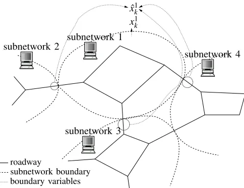
The basic idea for the parallelization is to utilize the possibility that a traffic network can be simulated in par-allel. A natural way to parallelize the simulation of traffic is to divide the traffic network into several subnetworks (corresponding to geographical regions), where each PU is responsible for one subnetwork and the relevant vari-ables of the neighboring segments are communicated (as illustrated in Fig. 1). The state of the traffic network and the measurements can be correspondingly partitioned intoS

subvectorsxs_k,s=1, ...,Swithxk= [(x1k)

T

,(x2_k)T, . . . ,(xS_k)T]T_,

and zk = [(z1k)

T

,(z2_k)T, . . . ,(zS_k)T]T_{. The system (1)-(2) can}

now be described by

x_ks=f_ks(xs_k−1,xˆs_k−1,vs_k−1), (6)

zs_k=hs_k(xs_k,ns_k), (7)

wheres=1, ...,S, and the vector ˆxs_k

−1collects all neighboring

subnetwork 1 subnetwork 2

subnetwork 3

subnetwork 4

x1_k

ˆ

x1

k

roadway

subnetwork boundary boundary variables

Fig. 1. An example of partitioning a traffic network into subnetworks for parallelized simulation/particle filtering.

state variables that act as an input to subnetworks.Note that not all states of the neighboring networks are communicated, only the variables that serve as a input to subnetworks.

Note also that for (7) it is assumed that the measurements taken in a subnetwork only depend on the state in that subnetwork. This assumption holds for traffic since detectors typically measure the traffic variables at one given location. In addition we assume the independence of state noises between the subnetworks and of independence measurement noises between the subnetworks:

p(xk|xk−1) =

S

∏

s=1

p(xs_k|xs_k−1,xˆs_k−1), (8)

p(zk|xk) = S

∏

s=1

p(zs_k|xs_k). (9)

1) First approach: shared particles: In this approach the

PUs of different subnetworks share the same particlesxi_k, and the particles are partitioned into subparticlesxs,i

k correspond-ing to subnetwork s. The PU corresponding to subnetwork

s is responsible for the calculations for subparticles xs,i k . This approach is functionally equivalent to the centralized approach, as presented above, given that (8) and (9) hold.

In the state update step, the subparticlesxs,i

k are now drawn from the distribution q(xs_k|xs,i

k−1,xˆ

s,i k−1,z

s

k) which is based on local information only (including neighboring states). Now, choosing the proposal distribution q(xs_k|xs_k−1,xˆs_k−1,zs_k) such that (c.f. (8))

q(xk|xik−1,zk) =

S

∏

s=1

q(xs_k|xs,i k−1,xˆ

s,i k−1,z

s

k), (10)

and using (8)-(9) and the facts that

p(xs,i k |x

s,i k−1) =

I

∑

j=1

p(xs,i k |x

s,i k−1,xˆ

s,j k−1)p(xˆ

s,j k−1|x

s,i k−1),

p(xˆs,j k−1|x

s,i k−1) =

(

1 if i=j,

the weight update equation (5) can be rewritten as

wi_k∝wi_k−1 S

∏

s=1

ws,i

k−1 ,

∑

i

wi_k=1, (12)

ws,i k−1=

p(zs_k|xs,i k )p(x

s,i k |x

s,i k−1,xˆ

s,i k−1)

q(xs,i k |x

s,i k−1,xˆ

s,i k−1,zsk)

. (13)

The consequence of (12)–(13) is that the state and mea-surement update can be performed locally (divided over S

processors) except for the weight update.

For each time stepkin the PF the following communica-tion has to take place:

• The state variables ˆxs_k,₋i₁ at the boundaries have to be

sent to subnetworks.

• The weight update factors ws_k,₋i₁ can be calculated

lo-cally, and only the results need to be communicated to a central PU to determinewi_k.

• The centrally calculated weightswi_kare normalized, and

sent back to the local PUs (after resampling, when necessary).

• Resampling requires communication to a central PU

where all weights wp,i

k are collected and the wik are calculated according to (12). For the residual resam-pling [8] and the systematic resamresam-pling [1] methods it is not necessary to communicate the particles themselves, since these methods use only the weights as the input and produce as a result the new particles as a selection from the existing old ones (with some selected multiple times, others not at all). Therefore, after resampling only the indices describing the selection are communicated back to the PUs. For the resampling algorithms that create particles at new locations in the state space, such as regularization [5] and the MCMC scheme [3] the particles themselves also have to be communicated, and consequently more communication is necessary. The pseudo code for the algorithm is given by ‘PF1’ in the frame below.

2) Second approach: separate particles: In this approach

the particles of the different subnetworks are not shared, only the statistics of the neighboring traffic state is communicated over the boundaries to each subnetworks. Consequently (11) does not hold anymore, but instead

p(xs,i k |x

s,i k−1) =

Z

ˆ

xs,j

k−1

{p(xs,i k |x

s,i k−1,xˆ

s,j k−1)p(xˆ

s,j k−1|x

s,i k−1)}dxˆ

s,j k−1.

(14)

Applying Monte-Carlo sampling to the product

p(xs,i k |x

s,i k−1,xˆ

s k−1)p(xˆ

s k−1|x

s,i

k−1) with a proposal distribution

q(xˆs_k−1|xs,i

k−1)results in the approximation

p(xs,i k |x

s,i k−1)≈

∑

j p(xs,i

k |x s,i k−1,xˆ

s,j k−1)p(ˆx

s,j k−1|x

s,i k−1)

q(ˆxs,j k−1|x

s,i k−1)

. (15)

Note that since the pdf of the communicated state variables is independent ofxs,i

k−1 (by assumption),

p(xˆs,j k−1|x

s,i

k−1) =p(ˆx

s,j

k−1). (16)

[{xi_k,wi_k}I

i=1] = PF1[{xik−1,w

i k−1}

I i=1,zk]

fors=1 :S (for each subnetwork simultaneously) do

fori=1 :I (for each particle)do

- Drawxs,i

k ∼q(xsk|x s,i k−1,xˆ

s,i k−1,z

s k)

- Determine the weight update factors according to (13) and send them to the central PU. At the central PU:

- Determinewi_k according to (12). - Normalize weights,wi_k=wi_k/∑iwik

ifIceff_<Ithreshold _then

- Resample particles (determine the mapping

ij) end

- Sendij andwi_k to each local PU. end

end

fors=1 :S (for each subnetwork) do

- Update the particles according to

xs,j k ←x

s,i

j

k , j=1, . . . ,I.

- Calculate the estimate of the state of subnetworks:E[xs_k] =∑I_i=1wikx

s,i k .

end

[{xi

k,wik}Ii=1] = PF2[{xik−1,wik−1}Ii=1,zk]

fors=1 :S (for each subnetwork) do

fori=1 :I (for each particle)do

- Draw ˆxs,ji k−1∼p(ˆx

s k−1)

- Drawxs,i k ∼q(x

s,i k |x

s,i k−1,xˆ

s,ji k−1,z

s k)

- Determine the weight update factors according to (18).

- Normalize weights,ws,i k =w

s,i k /∑iw

s,i k

ifIdeff,s<Ithreshold,s then - Resample particles. end

- Calculate the estimate of the state of subnetworks:E[xs_k] =∑I_i=1w

s,i k x

s,i k .

end end

Using this relation and taking only one sample from ˆxs,ji k−1∼

p(xˆs_k

−1)for eachi,and choosingq(xˆ

s,j k−1|x

s,i k ) =p(xˆ

s,j k−1),(15)

simplifies to

p(xs,i k |x

s,i

k−1)≈p(x

s,i k |x

s,i k−1,xˆ

s,ji

k−1). (17)

In this approach the weights are updated locally since there are no centralized particles (c.f. (12)):

ws,i k =w

s,i k−1

p(zs,i k |x

s,i k )p(x

s,i k |x

s,i k−1,xˆ

s,ji k−1)

q(xs,i k |x

s,i k−1,xˆ

s,ji k−1,z

s k)

. (18)

This form means for the particle filter that first ˆxs,ji k−1 needs

to be sampled from p(ˆxs_k

−1) and then x

s,i

k according to the the importance densityq(xs,i

k |x s,i k−1,xˆ

s,ji k−1,z

s

k).The algorithm is

In this approach there is no central PU, and there is only communication between the neighboring PUs. The commu-nication takes place in each time step when the neighboring state variables ˆxs,ji

k−1 are sent to subnetwork s, after these

quantities are drawn from ˆxs,ji k−1∼p(xˆ

s

k−1). In this approach

resampling does not require communication since it can be performed locally at each PU.

The advantages of this approach over the approach where the particles are shared are the following:

• it can be expected that this approach requires less

par-ticles since the dimension of the state space is reduced by a factor S (assuming that all subnetworks have the same number of states).

• for each subnetwork a different number of particles can

be used. This can be an advantage when a different accuracy is required for the different subnetworks. A disadvantage of this approach is that an approximation is introduced in the interaction (joint pdf) of the local states with the states in neighboring subnetworks (as given by (16)).

III. BENCHMARK

In this section we apply the developed parallelized particle filters to a benchmark problem consisting of state tracking of a freeway link consisting of two sublinks. The purpose of this benchmark is to compare the estimation accuracy, computational load and communication requirements for the centralized PF and the two parallelization approaches.

The benchmark network is small, but the same approach can be applied to networks of any size. Before the pre-sentation of the benchmark problem, the freeway model is described here.

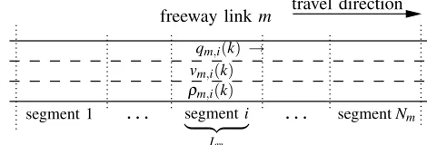
3) Freeway model – the METANET model: Consider a

freeway link m that is subdivided into Nm segments, each with a length Lm and λm lanes, and a discrete time step with lengthT (h). Traffic dynamics is described in terms of the aggregated variables speed vm,i(k) (km/h), flow qm,i(k) (veh/h), and density ρm,i(k) (veh/km/lane), where i is the segment index. In Fig. 2 the relevant variables are shown.

The METANET model equations are given by the funda-mental relationship between speed, density and flow

qm,i(k) =ρm,i(k)vm,i(k)λm, (19)

the law of conservation of vehicles

ρm,i(k+1) =ρm,i(k)

+ T

Lmλm

(qm,i−1(k)−qm,i(k)) +ξ

ρ

m,i(

k) (20)

and a heuristic relationship of the speed dynamics

vm,i(k+1) =vm,i(k) +

T

τ(V(ρm,i(k))−vm,i(k))

+ T

Lm

vm,i(k) (vm,i−1(k)−vm,i(k))

− ηT

τLm

ρm,i+1(k)−ρm,i(k)

ρm,i(k) +κ

+ξv

m,i(k), (21)

V(ρm,i(k)) =vfree,mexp

− 1

am

_ρ

m,i(k)

ρcrit,m

am

, (22)

whereξρ

m,i(k),andξ v

m,i(k)are random variables representing the random (unmodeled) dynamics in the speed and density evolution. Although (20) is an exact relationship and there-fore modeling error is not present, we include the random variableξρ

m,i(

k), to allow a state filter to correct the number of vehicles in the network. This noise model formulation is the same as in [17] and [7]. Furthermore,vfree,mis the free-flow speed in segment m, ρcrit,m is the critical density (the density at or above which traffic becomes unstable), andτ,

η,am,κ, are model fitting parameters without direct physical meaning.

An extension was introduced to be able to express the different anticipation behavior of the drivers at the head and the tail of a traffic jam (i.e., a shock wave) [6]. The parameter η in (21) is replaced by the density dependent

ηm,i(k)according to:

ηm,i(k) =

(

ηhigh ifρm,i+1(k)≥ρm,i(k)

ηlow ifρm,i+1(k)<ρm,i(k).

A. Boundary conditions

The variables qm,0,vm,0,ρm,Nm+1 areboundary variables which incorporate the influence of upstream and downstream segments from the considered link. Usuallyqm,0andvm,0can be measured directly, whereas in practice the densityρm,N+1 is not measured directly and must be estimated. Even though

qm,0 and vm,0 can be measured directly, the measurements will be corrupted by errors. Therefore, we will consider all boundary variables as extra states of the system and we will estimate them from the measurement data, similarly to the other state variables. This approach is also recommended in [17]. The dynamic evolution of the boundary variables is described by a random walk:



 qm,0(k+1)

vm,0(k+1)

ρm,Nm+1(k+1)

 =



 qm,0(k)

vm,0(k)

ρm,NM+1(k)

 +

 

ξ_mq

,0(

k)

ξv

m,0(k)

ξρ

m,NM+1(k)

 , (23)

where ξ_mq

,0(

k),ξv m,0(k),ξ

ρ

m,Nm+1(

k)are stochastic variables.

B. Measurements

The most frequently used traffic measurement devices typically measure speed and flow. For the segments that are

travel direction freeway linkm

.

.

.

.

.

.

segment 1 segmenti

| {z }

Lm

segmentNm

qm,i(k) →

ρm,i(k) vm,i(k)

equipped with sensors the measurement equations are:

yq_m

,i(

k) =qm,i(k) +n q m,i(

k), (24)

yv_m

,i(k) =vm,i(k) +n v

m,i(k), (25)

where nq_m

,i(k), and n v

m,i(k) are the measurement noises for the flow and the speed respectively.Note that in practice, traffic systems provide measurements with a larger sampling time than the model time step. Typically the measurement sampling time step is 1 or 5 minutes, while the model time step is 10s. Including this fact in the development of a PF is straightforward, but for the sake of simplicity we assume that each model time step a measurement is available.

C. State space representation

To bring equations (19)–(23) into the state-space represen-tation required by the various filters, the statexkis defined as2 xk= [ρ1(k), . . . ,ρN(k),v1(k), . . . , vN(k),v0(k),q0(k),ρN+1]T,

and the measurement vectorz_k= [yq_m

,i(

k)T_,yv m,i(

k)T_]T _collects the flow and speed measurements from (24) and (25) for the segments equipped with sensors.

D. Experiment design

1) Lay-out: The benchmark network consists of a 2-lane

freeway link of 10 segments of 1 km each. For the two parallel approaches this link is divided into two sublinks (“subnetworks”) consisting of respectively the first and the last five segments.

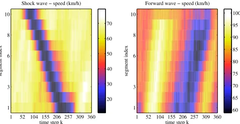
2) Scenario: Two different scenarios are used to

eval-uate the filters: one with downstream propagating waves (in free-flow) and one with an upstream propagating shock wave as shown in Fig. 3. These scenarios are de-fined by selecting the upstream and downstream bound-ary conditions. The motivation to select these two sce-narios is to have both conditions where information prop-agates forward and where information propprop-agates back-ward over the sublink boundaries. The state and mea-surement noises are taken to be Gaussian (although any other distribution could be taken) with state noise variances, var(ξv

m,i(k)) =0.5 (km/h)

2_,var(ξρ

m,i(k)) =0.5 (veh/km/lane)

2_,

and measurement noise variances var(nv_m

,i(

k)) =4 (km/h)2, and var(nq_m

,i(k) =22500 (veh/h)

2_.

3) Parameters: The following model parameters are used:

T =10 s, τ=18 s, a=1.867, ηhigh=65 km2/h, ηlow =

30 km2_{/h, κ =40 veh/km/lane, ρ}

crit,m=33.5 veh/km/lane,

v_min=7 km/h,v_free,m=102 km/h.

4) Detector configurations: Several detector

configura-tions are investigated. Segments that have detectors provide speed and flow measurements. For most experiments it is assumed that all segments are equipped with detectors.

For the experiment investigating the information exchange over the subnetwork boundaries it was assumed that seg-ments 1 and 10 are measured (the two ends of the complete link), and only the segments of the downstream sublink (sublink 2) are measured for the shock wave scenario. In

2

The link indexmis omitted in the rest of this section assuming that all the variables introduced hereafter refer to the same link.

1 52 104 155 206 257 309 360 1

3 6 8 10

Shock wave − speed (km/h)

time step k

segment index

20 30 40 50 60 70

1 52 104 155 206 257 309 360 1

3 6 8 10

Forward wave − speed (km/h)

time step k

segment index

60 65 70 75 80 85 90 95 100

Fig. 3. The shock wave (left) and the forward wave (right) scenario, used for the evaluation of the filters. The travel direction is from segment 1 to 10. The colors indicate the speed. Please note the difference in color bar scales: the shock wave scenario includes a wider range of speed since it also contains congested traffic.

this way the upstream sublink gets information about the incoming backward propagating shock wave only from the downstream sublink and not from the measurements, and the performance of the upstream link will depend on the information from the downstream neighbor link.

Similarly for the forward wave scenario only the upstream sublink is measured (and segment 10), to investigate the communication over the sublink boundary in case of a forward propagating wave (corresponding to downstream propagating information).

5) Filter setup: The particle filters are set up

accord-ing to the algorithms in Section II-A and II-B. For the proposal distribution the prior is used, and the filters are investigated for several numbers of particles in the range

I∈ {20,50,100,200,500,1000}. The resampling threshold is chosen to beIthreshold_{=0.3. The state noise v}i

k, which is sampled during the operation of the filters, is taken to have the same realization for the three different filters, for better comparability.

6) Performance measures: The performance of the filters

is evaluated by the following three performance measures:

• Tracking accuracy.For each filter the root mean square

error (RMSE) is determined of the expected value of the particles ˜xk=E(xik) relative to the states ˆxk in the reference scenarios. The RMSE is determined for the speed and the density separately, according to

JRMSE,ρ =

s

(ρˆi,k−ρ˜i,k)

2

KNm

,

where ˆρi,k and ˜ρi,k are the density components of respectively the real state and the expected state of the particles for segment iat time k, andK is the number of simulation steps.JRMSE,vis calculated similarly.

• Communication.The communication needs of the

weights between the PUs, and the communication of the weights to and from the central PU.

• CPU time.As a measure for the computational demand

the time that each filter needs for a complete run is determined.

IV. RESULTS& DISCUSSION

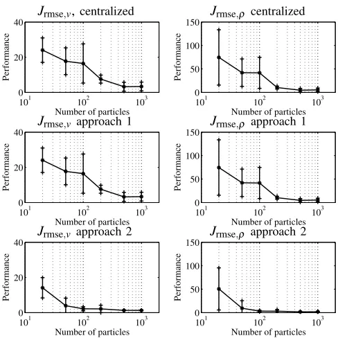
Fig. 4 shows the results for the tracking accuracy as a function of the number of particles, for the centralized filter (top), approach 1 (middle), and approach 2 (bottom). In these experiments all segments were measured and the shock wave scenario was used. The experiments were repeated 10 times and the figure shows the averages and the standard deviations of these experiments. For all filters the performance get better (lower error) when the number of particles increases. The performance of the centralized filter and the performance of approach 1 is equal because the two filters are functionally equivalent and the same noise realization is used.

Interestingly, the average performance of approach 2 is significantly better for all numbers of particles. From this it can be concluded that the improvement following from the fact that the same number of particles covers a smaller state space (i.e., a state space with lower dimensions) is more important than the deterioration following from the approximation of the pdf’s made at the boundaries of the sublinks.

Since there is no visible improvement between I=500 andI=1000 we selectI=500 for the other experiments.

Fig. 5 shows the CPU time needed by the different filters to complete a full scenario, as a function of the number of particles, again averaged over 10 runs. The averaging is necessary here as the measured CPU time may vary with some internal operations of the PC, such as memory swapping. The simulations were executed on a 2800 MHz Intel Pentium IV PC.

The shown values are normalized by the number of parti-cles, and the curves are nearly flat which indicates that the required CPU depends linearly on the number of particles (as expected). For both parallelization approaches the CPU time required by one of the PUs corresponding to one sublink, is clearly less than the CPU of the centralized filter. However, based on the number of floating point operations it would be expected that the parallelized filters have a computational demand around 50% of the centralized filter since the same operations are executed by 2 PUs instead of 1. The difference between the expectation and the simulation results can be explained by the overhead CPU time that is needed by all filters during code execution, such as the time needed to call the state transition functions, which is called the same number of times for all PUs. For larger problems it can be expected that the CPU time will not be dominated by this common overhead and the efficiency improvement will be higher.

The effect of the approximation introduced in approach 2 is investigated by the experiments with the shock wave and the forward wave scenarios. The detector locations are selected such that there are no detectors near the boundary in

101 102 103 0

20 40

Number of particles

Performance

101 102 103 0

50 100 150

Number of particles

Performance

101 102 103 0

20 40

Number of particles

Performance

101 102 103 0

50 100 150

Number of particles

Performance

101 102 103 0

20 40

Number of particles

Performance

101 102 103 0

50 100 150

Number of particles

Performance

Jrmse,v,centralized Jrmse,ρ centralized

Jrmse,v approach 1 Jrmse,ρ approach 1

Jrmse,v approach 2 Jrmse,ρ approach 2

Fig. 4. The filter root mean square error as a function of the number of particles for the centralized filter (top), approach 1 (middle), and approach 2 (bottom). The dots connected by the solid line indicate the mean, and the vertical lines with the ‘+’-signs the standard deviation over the 10 experiments. All segments are measured. Note the logarithmic scale of the horizontal axis.

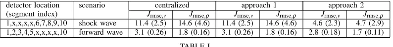
sublink 1 for the shock wave scenario, and no detectors near the boundary in sublink 2 for the forward wave scenario. In this way the information about the waves is communicated through the boundary of the two PUs and not via the measurements.

The performance of approach 2 is compared with the centralized filter (or the functionally equivalent approach 1) in Table I. Also in this case, the performance is averaged over 10 experiments and the standard deviation is shown in parentheses. The performance of approach 2 is significantly better, so we can conclude that the communication between the sublinks is sufficient to track forward and backward propagating waves.

Finally, the communication needs are shown in Table II. For the centralized filter only the measurements are commu-nicated, which are independent of the number of particles. For the parallelized approaches, communication also takes place between the boundary of the sublinks, and to the central PU in case of approach 1, which increases the communi-cation needs significantly. Nevertheless, these amounts of communication should not impose a problem for running these filters in real-time.

V. CONCLUSIONS

detector location scenario centralized approach 1 approach 2

(segment index) Jrmse,v Jrmse,ρ Jrmse,v Jrmse,ρ Jrmse,v Jrmse,ρ

1,x,x,x,x,6,7,8,9,10 shock wave 11.4 (2.5) 14.6 (4.6) 11.4 (2.5) 14.6 (4.6) 4.6 (2.3) 4.7 (2.9) 1,2,3,4,5,x,x,x,x,10 forward wave 3.1 (0.26) 1.8 (0.16) 3.1 (0.26) 1.8 (0.16) 2.8 (0.18) 1.7 (0.11)

TABLE I

TH E PERFORMANCE AND STANDARD DEVIATION(IN PARENTH ESES)FOR DIFFERENT DETECTOR LOCATIONS AND SCENARIOS,WITHI=500AND ALL

EXPERIMENTS ARE REPEATED10TIMES. TH E‘X’INDICATES AN UNMEASURED SEGMENT.

I centralized approach 1 approach 2

20 7180 57440 28720

50 7180 132830 61030

100 7180 258480 114880

200 7180 509780 222580

500 7180 1263680 545680

1000 7180 2520180 1084180

TABLE II

TH E NUMBER OF COMMUNICATED DOUBLES FOR EACH APPROACH AS A

FUNCTION OF TH E NUMBER OF PARTICLESI.

101 102 103

0 0.2 0.4 0.6 0.8 1

Number of particles

CPU time per particle (s/part)

centralized sublink 1 sublink 2 central PU

101 102 103

0 0.2 0.4 0.6 0.8 1

Number of particles

CPU time per particle (s/part)

centralized sublink 1 sublink 2

Fig. 5. The CPU time per particle for approach 1 (top) and approach 2 (bottom) as a function of the number of particles. The solid line is the CPU time for the centralized filter. All segments are measured. The simulations were executed on a 2800 MHz Intel Pentium IV PC. Note the logarithmic scale of the horizontal axis.

So the main conclusion is that despite the approximation used in approach 2, the performance of the filter was superior to the others for the experiments we carried out. Naturally, the communication needs of the parallelized approaches are higher than for the centralized filter, but the communication demand should not be a problem for the current data net-works.

VI. ACKNOWLEDGMENTS

Financial support by the project DWTC-CP/40 “Sustain-ability effects of traffic management”, sponsored by the Belgian government is gratefully acknowledged, as well as by the Belgian Programme on Inter-University Poles of Attraction V/22 on “Dynamical Systems and Control: Computation, Identification and Modelling” initiated by the Belgian State, Prime Minister’s Office for Science,

Technol-ogy and Culture.

REFERENCES

[1] S. Arulampalam, S. Maskell, N. Gordon, and T. Clapp. A tutorial on particle filters for on-line non-linear/non-Gaussian Bayesian tracking. IEEE Transactions on Signal Processing, 50(2):174–188, February 2002.

[2] M. Bolic, P.M. Djuric, and S. Hong. Resampling algorithms and archi-tectures for distributed particle filter. IEEE Trans. Signal Processing, 53:2442–2450, 2005.

[3] B. P. Carlin, N. G. Polson, and D. S. Stoffer. A Monte Carlo approach to nonnormal and non-linear state-space modelling. Journal of the American Statistical Association, 87(418):493 – 500, 1992. [4] C. Coates. Distributed particle filtering for sensor networks. InProc.

of the Int. Symp. Information Processing in Sensor Networks, Berkeley, California, April 2004.

[5] A. Doucet, J.F.G. de Freitas, and N.J. Gordon, editors. Sequential Monte Carlo Methods in Practice, chapter Improving Regularised Particle Filters. Springer-Verlag, New York, 2001.

[6] A. Hegyi, B. De Schutter, and J. Hellendoorn. Optimal coordination of variable speed limits to suppress shock waves. IEEE Transactions on Intelligent Transportation Systems, 6(1):102–112, March 2005. [7] A. Hegyi, D. Girimonte, R. Babuˇska, and B. De Schutter. A

comparison of filter configurations for freeway traffic state estimation. InProceedings of the International IEEE Conference on Intelligent Transportation Systems 2006, pages 1029–1034, Toronto, Canada, September 17–20 2006.

[8] J. S. Liu and R. Chen. Sequential Monte Carlo methods fory dynamical system. Journal of the American Statistical Association, 93:1032 – 1044, 1998.

[9] S. Maskell, K. Weekes, and M. Briers. Distributed tracking of stealthy targets using particle filters. InProc. of IEE seminar on target tracking: algorithms and applications, pages 13–20. IEE, Birmingham, UK, March 2006.

[10] L. Mihaylova and R. Boel. A particle filter for freeway traffic estimation. InProceedings of the 43rd IEEE Conference on Decision and Control, pages 2106–2111, Atlantis, Paradise Island, Bahamas, 2004.

[11] L. Mihaylova, R. Boel, and A. Hegyi. Freeway traffc estimation within particle filtering framework. Automatica, 43(2):290–300, 2007. [12] B. Ristic, S. Arulampalam, and N. Gordon.Beyond the Kalman filter.

Artech House, 2004. ISBN: 1-58053-631.

[13] X. Sheng, Y. H. Hu, and P. Ramanathan. Distributed particle filter with GMM approximation for multiple targets localization and tracking in wireless sensor network. In4th Intl. Conf. on Information Processing in Sensor Networks (IPSN), pages 181–188, 2005.

[14] X. Sun, L. Mu noz, and R. Horowitz. Mixture Kalman filter based highway congestion mode and vehicle density estimator and its application. InProceedings of the American Control Conference, pages 2098–2103, Boston, USA, 2004.

[15] Y. Wang and M. Papageorgiou. An adaptive freeway traffic state esti-mator and its real-data testing–Part I: Basic properties. InProceedings of the 8th International IEEE Conference on Intelligent Transportation Systems, pages 531–536, Vienna, Austria, September 13–16, 2005. [16] Y. Wang and M. Papageorgiou. An adaptive freeway traffic state

estimator and its real-data testing–Part II: Adaptive capabilities. In Proceedings of the 8th International IEEE Conference on In-telligent Transportation Systems, pages 537–548, Vienna, Austria, September13–16 2005.