Numerical Solution of Eighth Order Boundary Value
Problems by Galerkin Method with Quintic B-splines
K.N.S. Kasi Viswanadham
Department of Mathematics National Institute of Technology
Warangal- 506 004(INDIA)
Sreenivasulu Ballem
Department of Mathematics National Institute of Technology
Warangal- 506 004(INDIA)
ABSTRACT
In this paper, we present a finite element method involving Galerkin method with quintic B-splines as basis functions to solve a general eighth order two point boundary value problem.The basis functions are redefined into a new set of basis functions which vanish on the boundary where Dirichlet type of boundary conditions, Neumann boundary conditions, second order derivative boundary conditions and third order derivative type of boundary conditions are prescribed. The proposed method was applied to solve several examples of the eighth order linear and nonlinear boundary value problems. The solution of a nonlinear boundary value problem has been obtained as the limit of a sequence of solution of linear boundary value problems generated by quasilinearization technique. The obtained numerical results are compared with exact solutions available in the literature.
Keywords
Galerkin method; Quintic B-spline; Basis function; Eighth order boundary value problem; Absolute error.
1.
INTRODUCTION
In this paper, we consider a general eighth order linear boundary value problem given by
)
1
(
),
(
)
(
)
(
)
(
)
(
)
(
)
(
)
(
)
(
)
(
)
(
)
(
)
(
)
(
)
(
)
(
)
(
)
(
8 7
6
5 )
4 ( 4 )
5 ( 3
) 6 ( 2 )
7 ( 1 )
8 ( 0
d
x
c
x
b
y
x
a
x
y
x
a
x
y
x
a
x
y
x
a
x
y
x
a
x
y
x
a
x
y
x
a
x
y
x
a
x
y
x
a
subject to the boundary conditions
,
)
(
,
)
(
,
)
(
,
)
(
c
A
0y
d
C
0y
c
A
1y
d
C
1y
3 3
2
2
,
(
)
,
(
)
,
(
)
)
(
c
A
y
d
C
y
c
A
y
d
C
y
(2) where A0, C0, A1, C1, A2, C2, A3, C3 are finite real constants and a0(x), a1(x), a2(x), a3(x), a4(x), a5(x),a6(x), a7(x), a8(x), b(x) are all continuous functions defined on the interval [c, d]. Generally, this type of eighth order boundary value problems arises in the study of astrophysics, hydrodynamics and hydro magnetic stability, fluid dynamics, astronomy, beam and long wave theory, applied mathematics, engineering and applied physics. The boundary value problems of higher order differential equations have been investigated due to their mathematical importance and the potential for applications in diversified applied sciences. The literature on the numerical solutions of eighth order boundary value problems is very scarce. Chandra Sekhar [1] determined that when an infinite horizontal layer of fluid is heated from below and is under the
ordinary convection the ordinary differential equation is sixth order, when the instability sets in as overstability, it is modeled by an eight order ordinary differential equation. An eighth order differential equation derived from governing bending and axial vibrations by Shen [2], Paliwal and Pande [3] derived equations for the equilibrium in terms of displacement components for an orthotropic thin circular cylindrical shell subjected to a load that is not symmetric about the shell, which resulted in eighth order differential equations. The text book by Agarwal [4] contains theory which deals with the conditions for the existence and uniqueness of solutions of eighth order boundary value problems, though no numerical methods are given in for solving such problems. Solving such boundary value problems analytically is possible only in very rare cases. So, many numerical methods have been developed overs the years to approximate the solution for these types of boundary value problems. An eighth order differential equation occurs in torsional vibration of uniform beams was investigated by Bishop [5], Boutayes and Twizell [6] developed finite difference methods for the special case solution of the eighth order boundary value problems, Twizell et. al. [7] developed numerical methods for eighth, tenth, twelfth order eigenvalue problems arising in thermal instability, Inc and Evans [8] presented the solution of special case of eighth order boundary value problems using Adomain decomposition method, Siddiqi et. al. [9] presented solution of special case of eighth order boundary value problems using variational iterational technique, Ghazala Akram and Hamood Ur Rehman [10] presented the solution of special case of eighth order boundary value problems using kernel space method there were used searching least square value method investigated for nonlinear eighth order boundary value problems, Liu and Wu [11] presented the solution of special case of eighth order boundary value problems using generalized differential quadrature rule, Koonprasert and Torvattanabum [12] presented variational iterational method for solving eighth order boundary value problems, Javidi and Golbai [13] presented HPM for solution of eighth order boundary value problems, Prorshouhi at. al. [14] presented variatonal iterational method for solution of special case of eighth order boundary value problems.
In this paper, we try to present a simple finite element method which involves Gelerkin approach with quintic B-splines as basis functions to solve the eighth order two point boundary value problems of the type (1)-(2). This paper is organized as follows. Section 2, deals with the justification for using Galerkin method. In Section 3, a description of Galerkin method with quintic B-splines as basis functions is explained. In particular, we first introduce the basic concept of quintic B-splines and followed by the proposed method. In Section 4, the procedure to solve the nodal parameters has been presented. In section 5, the proposed method is tested on several linear and nonlinear boundary value problems. The solution to a nonlinear problem has been obtained as the limit of a sequence of solution of linear problems generated by the quasilinearization technique [19]. Finally, in the last section, the conclusions are presented.
2.
JUSTIFICATION FOR USING
GALERKIN METHOD
For the few decades, the finite element method has become very powerful, useful tool to solve the boundary value problems in the complex dynamical systems. In finite element method (FEM) the approximate solution can be written as a linear combination of basis functions which constitute a basis for the approximation space under consideration. FEM involves variational methods like Rayleigh Ritz, Galerkin, Petrov-Galerkin, Least Squares and Collocation etc.
In Galerkin method, the residual of approximation is made orthogonal to the basis functions. When one uses Galerkin method, a weak form of approximation solution for a given differential equation exists and is unique under appropriate conditions [20,21] irrespective of properties of a given differential operator. Further, a weak solution also tends to a classical solution of given differential equation, provided sufficient attention is given to boundary conditions [22]. That means the basis functions should vanish on the boundary where the Dirichlet type of boundary conditions are prescribed. Hence in this paper we employed the use of Galerkin method with quintic B-splines as basis functions to approximate the solution of eighth order boundary value problems.
3.
DESCRIPTION OF THE METHOD
Definition of quintic B-spline:
The quintic B-splines are defined in [23-25]. The existence of quintic spline interpolate s(x) to a function in a closed interval [c, d] for spaced knots (need not be evenly spaced) of a partitiond
x
x
x
x
c
0
1
...
n1
n
is established by constructing it. The construction of s(x) is done with the help of the quintic B-splines. Introduce ten additional knots x-5, x-4, x-3, x-2, x-1, xn+1, xn+2, xn+3, xn+4 and xn+5 in such a way that x-5<x-4<x-3<x-2<x-1<x0 and xn<xn+1<xn+2<xn+3<xn+4<xn+5.Now the quintic B-splines
B
i(
x
)'
s
are defined by
otherwise
x
x
x
x
x
x
x
B
r i ir i
i r i
,
0
]
,
[
,
)
(
)
(
)
(
3 35 3
3
where
5
5
(
) ,
(
)
0,
r r
r
r
x
x
if x
x
x
x
if x
x
and
33
)
(
)
(
i
i r
r
x
x
x
where {B-2(x), B-1(x), B0(x), B1(x), B2(x), B3(x),…,Bn-1(x), Bn(x), Bn+1(x), Bn+2(x)} forms a basis for the space
S
5(
)
of quintic polynomial splines. Schoenberg [25] has proved that quintic B-splines are the unique nonzero splines of smallest compact support with the knots atx-5<<x-4<…<x0<x1<…<xn-1<xn<xn+1<xn+2 <…...<xn+5. To solve the boundary value problem (1) and (2) by the Galerkin method with quintic B-splines as basis functions, we define the approximation for y(x) as
2
2
)
(
)
(
n
j
j
j
B
x
x
y
(3) where
j,s
are the nodal parameters to be determined. In Galerkin method the basis functions should vanish on the boundary where the Dirichlet type of boundary conditions are specified. In the set of quintic B-splines{B-2(x), B-1(x), B0(x),…,Bn(x), Bn+1(x), Bn+2(x)}the basis functions B-2(x), B-1(x), B0(x), B1(x), B2(x), Bn-2(x), Bn-1(x), Bn(x), Bn+1(x) and Bn+2(x) do not vanish at one of the boundary points. So, there is a necessity of redefining the basis functions into a new set of basis functions which vanish on the boundary where the Dirichlet type of boundary conditions are specified. Since, we are approximating the eighth order boundary value problem by quintic B-splines polynomial, we redefine the basis functions into a new set of basis functions which vanish on the boundary where the Dirichlet type boundary conditions, Neumann boundary conditions, second order derivative boundary conditions and third order derivative type of boundary condiotions are prescribed. The procedure for redefining the basis functions is as follows.Using the definition of quintic B-splines and the Dirichlet boundary conditions of (2), the approximate solution at the boundary points can be written as
0 0 2 2 0 1 1 0
0 0 0 1 1 0 2 2 0
( )
( )
( )
( )
( )
( )
( )
A
y c
y x
B
x
B
x
B x
B x
B x
(4)0 2 2 1 1
1 1 2 2
( )
( )
( )
( )
( )
( )
( )
n n n n n n n
n n n n n n n n n
C
y d
y x
B
x
B
x
B x
B
x
B
x
(5)Eliminating
2 and
n2from the equations (3), (4) and (5), we get
11
1
(
)
(
)
)
(
n
j
j j
P
x
x
w
x
y
(6)where
)
(
)
(
)
(
)
(
)
(
22 0 2
0 2
0
1
B
x
x
B
C
x
B
x
B
A
x
w
nn n
and 0 2 2 0 2 2
( )
( )
( ),
1,0,1, 2
( )
( )
( ),
3,...,
3
(8)
( )
( )
( ),
2,
1, ,
1.
( )
j j j j j n j n n nB x
B x
B x
j
B x
P x
B x
j
n
B x
B x
B
x
j n
n
n n
B
x
Using the Neumann boundary conditions of (2) to the approximate solution y(x) in (6), we get
)
(
)
(
)
(
)
(
)
(
)
(
)
(
0 2 2 0 1 1 0 0 0 0 1 1 0 1 0 1x
P
x
P
x
P
x
P
x
w
x
y
c
y
A
(9))
(
)
(
)
(
)
(
)
(
)
(
)
(
1 1 1 1 2 2 1 1 n n n n n n n n n n n n n nx
P
x
P
x
P
x
P
x
w
x
y
d
y
C
(10)Eliminating
1and
n1 from the equations (6), (9) and (10), the approximation for y(x) can be written as
n j j jQ
x
x
w
x
y
0
2
(
)
(
)
)
(
(11)where ) ( ) ( ) ( ) ( ) ( ) ( ) ( ) ( 1 1 1 1 1 0 1 0 1 1 1
2 P x
x P x w C x P x P x w A x w x w n n n n (12) and n n n j x P x P x P x P n j x P j x P x P x P x P x Q n n n n j j j j j j , 1 , 2 ), ( ) ( ) ( ) ( ) 13 ( 3 ,..., 3 ) ( 2 , 1 , 0 ), ( ) ( ) ( ) ( ) ( 1 1 1 0 1 0
Using the second order derivative boundary conditions of (2) to the approximate solution y(x) in (11), we get
) ( ) ( ) ( ) ( ) ( ) ( 0 2 2 0 1 1 0 0 0 0 2 0 2 x Q x Q x Q x w x y c y A
(14)) ( ) ( ) ( ) ( ) ( ) ( 1 1 2 2 2 2 n n n n n n n n n n n x Q x Q x Q x w x y d y C
(15)
Eliminating
0and
n from the approximations (11), (14) and (15), the approximation for y(x) can be written as
1 13
(
)
(
)
)
(
n
j j j
R
x
x
w
x
y
(16) where ) ( ) ( ) ( ) ( ) ( ) ( ) ( )( 0 2 2
0 0 0 2 2 2
3 Q x
x Q x w C x Q x Q x w A x w x w n n n n 0 0 0 0
( )
( )
( ) ,
1, 2
( )
( )
( ) ,
3,...,
3
(18)
( )
( )
( ) ,
2,
1.
( )
j j j j j n j n n nQ x
Q x
Q x
j
Q x
R x
Q x
j
n
Q x
Q x
Q x
j
n
n
Q x
Using the third order derivative boundary conditions of (2) to the approximate solution y(x) in (16), we get
)
(
)
(
)
(
)
(
)
(
0
2
2
0
1
1
0
3
0
3
x
R
x
R
x
w
x
y
c
y
A
(19))
(
)
(
)
(
)
(
)
(
1
1
2
2
3
3
n
n
n
n
n
n
n
n
x
R
x
R
x
w
x
y
d
y
C
(20)Eliminating
1and
n1 from the equations (11), (14) and (15), the approximation for y(x) can be written as2 2
( )
( )
( )
n j j jy x
w x
B x
(21)where
)
(
)
(
)
(
)
(
)
(
)
(
)
(
)
(
1
1
3
3
1
0
1
0
3
3
3
x
R
x
R
x
w
C
x
R
x
R
x
w
A
x
w
x
w
n
n
n
n
(22) and
(
)
(
),
2
)
(
)
(
3
,...,
3
),
(
2
),
(
)
(
)
(
)
(
)
(
~
1 1 1 0 1 0n
j
x
R
x
R
x
R
x
R
n
j
x
Rj
j
x
R
x
R
x
R
x
R
x
B
n n n n j j j j j (23) Now the new set of basis functions for the approximation y(x)is{ ( ), 2,..., 2} j
B x j n . Applying the Galerkin method to (1) with a new set of basis functions, we get
0
0
(8) (7) (6)
0 1 2
(5) (4)
3 4 5
6 7 8
( )
( )
( )
( )
( )
( )
( )
( )
( )
( )
( )
( )
( )
( )
( ) ( )
( ) ( )
( )
( )
( )
2, 3,...
2
(24)
[
]
n n x x i x i xa x y
x
a x y
x
a x y
x
a x y
x
a x y
x
a x y
x
a x y x
a x y x
a x y x
B x dx
b x B x dx for i
n
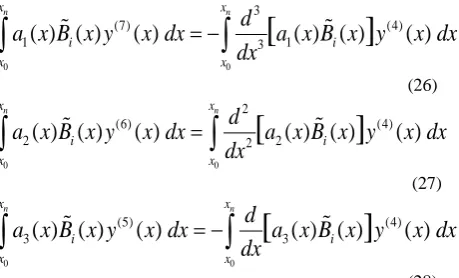
Integrating by parts the first four terms on the left hand side of (24) and after applying the boundary conditions prescribed in (2), we get
4
(8) (4)
0
( ) ( )
( )
[
0( ) ( )
]
( )
n n
x x
i i
d
a x B x y
x dx
a x B x y
x dx
(25)
0 0
3
(7) (4)
1
( ) ( )
( )
3[
1( ) ( )
]
( )
n n
x x
i i
x x
d
a x B x y
x dx
a x B x y
x dx
dx
(26)
0 0
2
(6) (4)
2
( ) ( )
( )
2[
2( ) ( )
]
( )
n n
x x
i i
x x
d
a x B x y
x dx
a x B x y
x dx
dx
(27)
0 0
(5) (4)
3
( ) ( )
( )
[
3( ) ( )
]
( )
n n
x x
i i
x x
d
a x B x y
x dx
a x B x y
x dx
dx
(28) Substituting (25), (26), (27), (28) in (24) and using the approximation for y(x) given in (21), and after rearranging the terms for resulting equations, the resulting system of equations can be written in the matrix form as
A
B
(29)where
A
[
a
ij];
0
4 3
0 1
4 3
2
2 3
2
(4)
4 5
6 7
8
{[
( ( ) ( ))
( ( ) ( ))
( ( ) ( ))
( ( ) ( ))
( ) ( )]
( )
( ) ( )
( )
( ) ( )
( )
( ) ( )
( )
( ) ( ))
( )}
n
x
ij i i
x
i i
i j i j
i j i j
i j
d
d
a
a x B x
a x B x
dx
dx
d
d
a x B x
a x B x
dx
dx
a x B x B
x
a x B x B x
a x B x B x
a x B x B x
a x B x B x dx
for i =2,3,…n-2; j =2,3,…,n-2 (30)
[ ];
b
i
B
0
4
0 4
3 2
1 2
3 2
(4)
3 4
5 6
7 8
{ ( )
( ) [
(
( )
( ))
( ( )
( ))
(
( )
( ))
( ( )
( ))
( )
( )]
( )
( )
( )
( )
( )
( )
( )
( )
( )
( )
( )
( )) ( )}
n
x
i i i
x
i i
i i
i i
i i
d
b
b x B x
a x B x
dx
d
d
a x B x
a x B x
dx
dx
d
a x B x
a x B x w
x
dx
a x B x w x
a x B x w x
a x B x w x
a x B x w x dx
for i = 2,3,…,n-2 (31)
and
[
2 3
n2]
T4.
PROCEDURE TO FIND A SOLUTION
FOR NODAL PARAMETERS
A typical integral element in the matrix
A
is 10 n
m m
I
where m1
( ) ( ) ( )
m
x
m i j
x
I
r x r x Z x dx
andr x
i( ),
( )
jr x
are the quintic B-spline basis functions or their derivatives. It may be noted thatI
m
0
if3 3 3 3 1
(
x
i,
x
i)
(
x
j,
x
j)
(
x
m,
x
m)
. Toevaluate each
I
m, we employed 6-point Gauss-Legendre quadrature formula. Thus the stiffness matrixA
is an eleven diagonal band matrix. The nodal parameter vector
has been obtained from the systemA
B
by using a band matrix solution package. We have used the FORTRAN-90 program to solve the boundary value problems (1)-(2) by the proposed method.5.
NUMERICAL RESULTS
To demonstrate the applicability of the proposed method for solving the eighth order boundary value problems of the types (1) and (2), we considered three linear boundary value problems and two nonlinear boundary value problems. Numerical results for each problem are presented in tabular forms and compared with the exact solutions available in the literature.
Example 1: Consider the linear boundary value problem
y
(8)
16
y
4,
1
x
1
(32) subject toy
( 1)
y
(1)
0
,sinh 2 sin 2
( 1)
(1)
.25
cosh 2 cos 2
y
y
,( 1)
(1)
0,
y
y
sin1cos1 cosh1sinh1
( 1)
(1)
cos 2 cosh 2
y
y
.The exact solution for the above problem is
y(x)=25[1-2(sin 1 sinh1 sin x sinh x + cos 1 cosh1 cos x cosh x)/(cos 2 + cosh x)]
[image:4.595.57.287.84.223.2]Table 1. Numerical results for Example 1 x Exact Solution Absolute Error by
proposed method
-0.8 -0.6 -0.4 -0.2 0.0 0.2 0.4 0.6 0.8
3.976926E-02 7.498498E-02 1.023106E-01 1.195382E-01 1.254157E-01 1.195382E-01 1.023106E-01 7.498498E-02 3.976926E-02
6.705523E-08 1.654029E-06 4.455447E-06 6.906688E-06 7.852912E-06 6.698072E-06 3.896654E-06 1.467764E-06 3.725290E-07
Example 2: Consider the linear boundary value problem
y
(8)
xy
(48 15
x x e
3) ,
x0
x
1
(33)subject to
y
(0)
y
(1)
0,
y
(0) 1,
y
(1)
e
,
(0)
0,
y
y
(1)
4 ,
e
(0)
3,
y
y
(1)
9 .
e
[image:5.595.310.547.161.302.2]The exact solution for the above problem is y =x(1-x)ex. The proposed method is tested on this problem where the domain [0, 1] is divided into 10 equal subintervals. The obtained numerical results for this problem are given in Table 2. The maximum absolute error obtained by the proposed method is 1.227856x10⁻⁵.
Table 2. Numerical results for Example 2 x Exact Solution Absolute Error by
proposed method
0.1 0.2 0.3 0.4 0.5 0.6 0.7 0.8 0.9
9.946539E-02 1.954244E-01 2.834704E-01 3.580379E-01 4.121803E-01 4.373085E-01 4.228881E-01 3.560865E-01 2.213642E-01
5.215406E-08 2.220273E-06 7.003546E-06 1.114607E-05 1.227856E-05 8.881092E-06 2.533197E-06 1.817942E-06 2.041459E-06
Example 3: Consider the linear boundary value problem
1
0
,
sin
4
sin
16
cos
14
2
2
2
2
2
(
6
)
(
5
)
(
4
)
)
7
(
)
8
(
x
x
x
x
x
y
y
y
y
y
y
y
y
y
(34) subject to
y
(0)
0,
y
(1)
0,
(0)
1,
y
y
(1)
2sin1,
(0)
0,
y
y
(1)
4cos1 2sin1,
y
(0)
7,
(1)
6 cos1 6sin1.
y
The exact solution for the above problem is 2
( )
(
1) sin .
y x
x
x
The proposed method is tested on this problem where the domain [0, 1] is divided into 10 equal subintervals. The obtained numerical results for this problem are given in Table 3. The maximum absolute error obtained by the proposed method is 7.688999x10⁻⁶.Table 3. Numerical results for Example 3 x Exact Solution Absolute Error by
proposed method
0.1 0.2 0.3 0.4 0.5 0.6 0.7 0.8 0.9
-9.883508E-02 -1.907226E-01 -2.689234E-01 -3.271114E-01 -3.595692E-01 -3.613712E-01 -3.285510E-01 -2.582482E-01 -1.488321E-01
3.799796E-07 2.145767E-06 5.632639E-06 9.745359E-06 1.138449E-05 1.013279E-05 7.271767E-06 3.874302E-06 1.430511E-06
Example 4: Consider the nonlinear boundary value problem
y
(8)
e y
x 2
e
x
e
3x,
0
x
1
(35)
subject to
y
(0)
1,
y
(1)
e
1,
y
(0)
1,
1
(1)
,
y
e
1(0)
1,
(1)
,
y
y
e
1
(0)
1,
(1)
.
y
y
e
The exact solution for the above problem is y=e-x. The nonlinear boundary value problem (35) is converted into a sequence of linear boundary value problems generated by quasilinearization technique [19] as
(8) 2 3
( 1)
[2
( )]
( 1)[
( )]
x x x x
n n n n
y
y e
y
y
e
e
e
forn=0,1,2,…
(36)
subject to
y
(n1)(0)
1,
y
(n 1)(1)
1
,
e
( 1) ( 1)
1
(0)
1,
(1)
,
n n
y
y
e
(n 1)
(0)
1,
y
( 1)1
(1)
,
n
y
e
(n 1)
(0)
1,
y
( 1)1
(1)
.
n
y
e
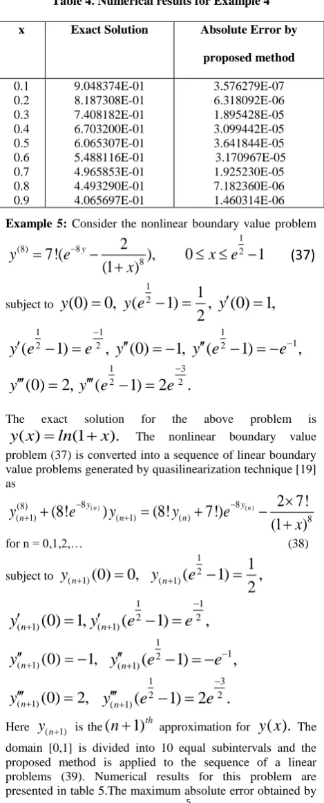
[image:5.595.316.539.331.617.2]Table 4. Numerical results for Example 4 x Exact Solution Absolute Error by
proposed method
0.1 0.2 0.3 0.4 0.5 0.6 0.7 0.8 0.9
9.048374E-01 8.187308E-01 7.408182E-01 6.703200E-01 6.065307E-01 5.488116E-01 4.965853E-01 4.493290E-01 4.065697E-01
3.576279E-07 6.318092E-06 1.895428E-05 3.099442E-05 3.641844E-05 3.170967E-05 1.925230E-05 7.182360E-06 1.460314E-06
Example 5: Consider the nonlinear boundary value problem
1
(8) 8 2
8
2
7!(
),
0
1
(1
)
y
y
e
x
e
x
(37)
subject to
y
(0)
0,
12
1
(
1)
,
2
y e
y
(0) 1,
1 1
2 2
(
1)
,
y e
e
y
(0)
1,
y e
(
12
1)
e
1,
1 3
2 2
(0)
2,
(
1)
2
.
y
y e
e
The exact solution for the above problem is
( )
(1
).
y x
ln
x
The nonlinear boundary value problem (37) is converted into a sequence of linear boundary value problems generated by quasilinearization technique [19] as( ) ( )
8 8
(8)
( 1) ( 1) ( ) 8
2 7!
(8!
)
(8!
7!)
(1
)
n n
y y
n n n
y
e
y
y
e
x
for n = 0,1,2,… (38)
subject to
y
(n1)(0)
0,
1 2 ( 1)
1
(
1)
,
2
n
y
e
1 1
2 2
(n1)
(0) 1,
(n 1)(
1)
,
y
y
e
e
(n 1)
(0)
1,
y
1
1 2
(n1)
(
1)
,
y
e
e
(n 1)
(0)
2,
y
1 3
2 2
(n 1)
(
1)
2
.
y
e
e
[image:6.595.50.285.77.659.2]Here
y
(n1) is the(
n
1)
th approximation fory x
( ).
The domain [0,1] is divided into 10 equal subintervals and the proposed method is applied to the sequence of a linear problems (39). Numerical results for this problem are presented in table 5.The maximum absolute error obtained by the proposed method is 1.00135x10⁻⁵.
Table 5. Numerical results for Example 5 x Exact Solution Absolute Error by
proposed method
0.1 0.2 0.3 0.4 0.5 0.6 0.7 0.8 0.9
6.285473E-02 1.219913E-01 1.778251E-01 2.307057E-01 2.809298E-01 3.287517E-01 3.743905E-01 4.180371E-01 4.598581E-01
2.011657E-07 4.544854E-07 1.519918E-06 4.068017E-06 6.705523E-06 9.059906E-06 1.001358E-05 5.453825E-06 2.592802E-06
6.
CONCLUSIONS
In this paper, a Galerkin method with quintic B-splines as basis functions to solve a general eighth order boundary value problem has been developed. The quintic B-splines basis set has been redefined into a new set of basis functions which vanish on the boundary where the Dirichlet boundary conditions, Neumann boundary conditions, secondary order derivative boundary conditions and third order derivative boundary conditions are prescribed. The proposed method has been tested on three linear and two nonlinear eighth order boundary value problems. The numerical results obtained by the proposed method are in good agreement with the exact solutions available in the literature. The objective of this paper is to present a simple and accurate method to solve a
general eighth order boundary value problem.
7.
REFERENCES
[1] Chandra, sekhar, S. 1981 Hydrodynamics and Hydromagnetic Stability. New York:Dover.
[2] Shen, Y. I. Hybrid damping through intelligent constrained layer layer treatments. ASME Journal of Vibration and Acoustics. 116(1994), 341-349.
[3] Paliwal, D. N., and Pande, A. Orthotropic cyclindrical presure vessels under line load. International Journal of Pressure Vessels and Piping. 76(1999), 455-459. [4] Agarwal, R. P. 1986 Boundary value problems for
higher order differential equations. World Scientific, Singapore.
[5] Bishop, R. E. D., Cannon, S.M., and Miao, S. On coupled bending and torsional vibration of uniform beams. Journal of Sound and Vibration. 131(1989), 457-464.
[6] Twizell, E. H., and Boutayeb, A. Finite-difference methods for the solution of special eighth-order boundary value problems. International Journal of Computer Mathematics. 48(1993), 63-75.
[7] Twizell, E. H., and Boutayeb, A. Numerical methods for eighth, tenth and twelfth-order eigenvalue problems arising in thermal instability. Advances in Computational Mathematics. 2(1994), 407-436. [8] Inc, M., and Evans, D. J. An efficient approach to
approximate solutions of eighth order boundary value problems. International Journal of Computer Mathematics. 81(2004), 685-692.
problems using Variational iteration technique. European Journal of Scientific Research. 30(2009), 361-379.
[10] Ghazala, Akram., and Hamood, Ur, Rehman. Numerical solution of eighth order boundary value problems in reproducing kernel space. Numerical Algorithm. 62(2013), 527-540.
[11] Liu, G.R., and Wu, T.Y. Diffrential quadrature solutions of eighth order boundary value differential equations. Journal of Computational and Applied Mathematics. 145(2002), 223-235.
[12] Torvattanabun, M., and Koonprasert, S. Variational iteration method for solving eighth order boundary value problems. Thai Journal of Mathematics. Special Issue(2010), 121-129.
[13] Golbabai., and Javidi, M. Application of homotopy perturbation method for solving eighth-order boundary value problems. Applied Mathematics and Computation. 191(2007), 334-346.
[14] Mehdi, Gholami, Porshokouhi., Behzad Ghanabari., et. al., Numerical solutions of eighth order boundary value problems with variation method. General Mathematics Notes. 2(2011), 128-133.
[15] Shahid, S.Siddiqi., and Ghazala, Akram. Solutions of eighth order boundary value problems using the non-polynomial spline technique. International Journal of Computer Mathematics. 84(2007), 347--368.
[16] Shahid, S. Siddiqi., and Ghazala, Akram. Nonic spline solutions of eighth order boundary value problems.
Applied Mathematics and Computation. 182(2006), 829-845.
[17] Twizell, E. H., and Siddiqi, S.S. Spline solutions of linear eight order boundary value problems. Computer Methods in Applied Mechanics and Engineering. 131(1996), 309-325.
[18] Kasi, Viswanadham, K. N. S., and Showri, Raju, Y. Quintic B-spline Collocation method for eighth boundary value problems. Advances in Computational Mathematics and its Applications. 1(2012), 47-52. [19] Kalaba, R. E., and Bellman, R. E. 1965
Quasilinearzation and nonlinear boundary value problems. American Elsevier, New York.
[20] Bers, L., John, F., and Schecheter, M. 1964 Partial differential equations. John Wiley Inter Science, New York.
[21] Lions, J. L., and Magenes, E. 1972 Non-Homogeneous boundary value problem and applications. Springer-Verlag, Berlin.
[22] Mitchel, A. R., and Wait, R. 1977 The finite element method in partial differential equations. John Wiley and Sons, London.
[23] Prenter, P. M. 1989 Splines and variational methods. John-Wiley and Sons, New York.
[24] Carl, de-Boor. 2001 A Pratical guide to splines. Springer-Verlag.