http://dx.doi.org/10.4236/ijaa.2015.53026
Mass Transfer in Binary Stellar Evolution
and Its Stability
Seblu Humne Negu, Solomon Belay Tessema
Astronomy and Astrophysics Research Division, Entoto Observatory and Research Center (EORC), Addis Ababa, Ethiopia
Email: [email protected], [email protected]
Received 30 May 2015; accepted 27 September 2015; published 30 September 2015
Copyright © 2015 by authors and Scientific Research Publishing Inc.
This work is licensed under the Creative Commons Attribution International License (CC BY).
http://creativecommons.org/licenses/by/4.0/
Abstract
The evolution of a binary star system by various analytical and numerical approximations of mass transfer rate normalized to the equilibrium rate and its stability conditions are investigated. We present results from investigations of mass transfer and stability in close binary star systems us-ing the different orbital parameters. The stability and instability of mass transfer in binary star evolution depends on the exchange of material which the response of the binary to the initial Roche lobe overflow causes the donor to loose even more material. Our work is mainly focused on basic mathematical derivations, analytical and numerical solutions in order to explain the mass transfer system in different orbital parameters as well as the results are compared with previous studies in both cases. Mass transfer is usually stable, as long as the winds specific angular mo-mentum does not exceed the angular momo-mentum per reduced mass of the system. This holds for both dynamical and thermal time scales. Those systems which are not stable will usually transfer mass on the thermal time scale. The variation of Roche lobe radius with mass ratio in the binary, for various orbital parameters in the conservative and non-conservative mass transfer, as well as the evolution equations, orbital angular momentum of the binary system and the corresponding analytical and numerical solutions for different cases, under certain restrictive approximations is derived, simulated and discussed.
Keywords
Mass Transfer, Binary Star, Stellar Evolution, Stability, Instability
1. Introduction
occurs in many different types of systems, to widely varying effects [1]. Contamination of the envelope of a less evolved star with chemically processed elements, as in Barium stars [2], and catastrophic mass transfer, by common envelope phase, as in W UMa systems; or a slow, steady mass transfer by Roche lobe overflow [2].
Close binary stars consisting of two compact stellar remnants (white dwarfs (WDs), neutron stars (NSs), or black holes (BHs)) are considered as primary targets of the forthcoming field of gravitational wave (GW) as-tronomy [3] since their orbital evolution has entirely controlled by the emission of gravitational waves and leads to ultimate coalescence (merger) of the components. GW emission is the sole factor responsible for the change of orbital parameters of a pair of compact (degenerate) stars. However, at the early stages of binary evolution, it is the mass transfer between the components and the loss of matter and its orbital angular momentum that play a dominant dynamical role.
Mass transfer is particularly interesting if one considers the evolution of a system with at least one degenerate star. In these cases, mass transfer produces spectacular effects, resulting in part from the intense magnetic and gravitational fields of the compact objects, pulsed X-ray emission, nuclear burning, novae outbursts, and so on. Also, since the mass transfer rates can be high and orbital period measurements accurate, one may see the dy-namical effects of mass transfer on the binary orbit, as in Cygnus X-3 [4].
In the case of cataclysmic variables (CVs) and low mass X-ray binary system (LMXBs), one has a highly evolved, compact star (CVs and LMXBs contain white dwarfs and neutron stars, respectively) and a less evolved main sequence or red giant star. Mass transfer usually proceeds by accretion onto the compact object, and is se-cularly stable. Most of these objects involve one component filling its Roche lobe (the donor or secondary), trans- ferring mass to a compact star (the accretor or primary) and the mass leaking out of the inner Lagrangian point forms an accretion disk around the accretor. A binary system starts out as detached [4] [5], with both stars in hy-drostatic equilibrium and filling an equipotential surface inside their Roche lobes. In a binary, both stars (1 and 2 can fill their Roche lobes at subsequent evolutionary stages). We use the convention which 1 denotes the primary star, and 2 denotes the secondary star of the binary. In this convention, the mass ratio is
2 1 d a 1
q=m m =m m > . During phases of mass transfer, we denote the mass-losing star, the “donor”, with sub-script “d” and the companion star, the “accretor”, with subscript “a”. The transfer will be accompanied by a stel-lar wind from the mass-losing star, or ejection of matter from the accretor, as in novae and galactic jet sources.
There are various unanswered questions in the evolution of LMXBs into low mass binary pulsars (LMBPs, in which a millisecond radio pulsar is in a binary with a low mass white dwarf companion) and of CVs. Among these are the problem of the disparate birthrates of the LMXBs and the LMBPs (Kulkarni and Narayan1988), es-timation of the strength of X-ray heating induced winds from the donor star.
Now, if a star is a member of a binary star system, then it is possible that as the components evolving, one of them (or both) can fill up its Roche lobe. Thomas (1977) classified mass transferring binaries on the basis of what state of evolution the donor is in as follows:
Case A: If the orbital separation is small enough (usually a few days), the star can fill its Roche lobe during its slow expansion through the main-sequence phase while still burning hydrogen in its core.
Case B: If the orbital period is less than about 100 days, but longer than a few days, the star will fill its Roche lobe during the rapid expansion to a red giant with a helium core. If the helium core ignites during this phase and the transfer is interrupted, the mass transfer is Case B.
Case C: If the orbital period is above 100 days, the star can evolve to the red supergiant phase before it fills its Roche lobe. In this case, the star may have a CO or ONe core.
Case A mass transfer occurs during the slow growth, Case B during the first rapid expansion, and Case C du- ring the final expansion phase. The nature of the remnant depends upon the state of the primary during the onset of RLOF and the orbital properties of the resultant binary depend upon the details of the mass transfer.
The problem of mass transfer in binaries by Roche lobe overflow has received a good deal of attention in the literature over the past few decades, typically in investigations of one aspect or another of orbital evolution or stability. [6] examined mass transfer by isotropic winds and accretion, in investigating the evolution of short pe-riod binary X-ray sources with extreme mass ratios, and developed models with accretion and (typically) iso-tropic re-emission of transferred matter, in the context of the period gap in cataclysmic variables.
transfer in binary stellar evolution using analytical and numerical methods which will give brief relations about stability and mass transfer.
The aim of this paper is to study mass transfer in binary stellar evolution behavior using mass transfer and different orbital parameters. This will be used to study stability properties of binary stars using analytical and numerical solutions. We calculate the rate of change of orbital angular momentum, orbital periods, angular speed and stability analysis of mass transfer rates, with relevant evolution in general form.
The paper is organized as follows:
In Section (2), we derive basic equations of mass transfer, mass transfer and evolution of orbital parameters, conservative and non-conservative mass transfer and evolution equations; in Section (3), stability analysis of mass transfer and its rate will be determined; in Section (4), analytical and numerical solutions will be presented. Finally our main conclusions are summarized in Section (5).
2. Basic Equations of Mass Transfer
2.1. Mass Transfer and the Evolution of Orbital Parameters
In this section, expressions for the variation of orbital parameters with loss of mass from one of the stars are de-rived. In what follows, the two stars will be referred to as m1 and m2, with the latter the mass losing star.
The angular momentum (AM) of binary component i in a circular orbit is expressed as:
J v a
i i i i i i i i
J = =m × =m v a (1) where vi=ωai is the velocity of accretor and donor star; “i” stands for the accretor “a” and donor “d” stars respectively, ai is the position of the accretor and donor star, and ω is the orbital angular spin frequency.
2 i i i J =m aω
Roche geometry changes are governed by the total orbital angular momentum J of the system which is given by
(
2 2)
21 2
a d a d T
J=J +J = m a +m a =µ ω µa = GM a (2) where aa =
(
md MT)
a a , d =(
ma MT)
a are the distance of the two stars from the center of mass (semi ma-jor-axis), µ =m ma d(
ma+md)
is the reduced mass, MT =ma+md is the total mass, and the mass ratio isd a
q=m m . Throughout this paper, we consider an eccentricity e will be zero.
The period “P”, the semi major axis “a” and the total mass transfer related through Kepler’s law as:
(
)
2 23
2π P GMT
a
ω
= = (3)
which implies that the orbital angular momentum J can be written as:
( )
22π a d
T PG
J P m m
M
=
(4)
The angular momentum for binary component “i” is given by
i i J J
m
µ
= (5)
and the specific angular momentum for binary component “i” can be written as:
2
i i i i
l =J m =µJ m (6) where mi is mass of the accretor and donor and li is specific angular momentum of the accretor and donor star, respectively.
From Kepler’s 3rd
3 2
~ 3a 2P M
a P M
a P M
∝ = + (7)
Hence from Equation (4) the orbital angular momentum J of a binary star is given by
(
)
1/ 2 2 1 a dGa e
J m m
M
−
=
(8)
In many cases the angular momentum stored in the rotation of the two stars is negligible compared to the or-bital angular momentum, so that Equation (8) also represents the oror-bital angular momentum of the binary, to good approximation. By differentiating this expression we obtain a general equation for the evolution of orbital parameters:
(
2)
1 1 1 2
2 2 2 1
a d
a d
m m
J a M ee
J =m +m = a− M− −e
(9)
and
(
2)
2 2
1
a d
a d
m m
a M J ee
a M J m m e
= + − + −
−
(10)
In Equation (10), e is a parameter that determines the amount by which its orbit around another body deviates from a perfect circle. From Equation (7) and Equation (10) the rate of change of orbital period, semi major axis, and total mass transfer can be written as:
3 1
2 2
P a M
P= a− M
or
d 3 d 1 d
d 2 d 2 d
p a M
p t = a t− M t (11)
which depends on time “t”.
By integrating Equation (11) we obtain:
3 0 0
0 M a
P P
a M
=
(12)
where P a0, 0, andM0 are initial orbital period, semi major axis, and total mass transfer of the binary stars, re-spectively.
In the case of Roche lobe overflow in an already circularized binary, the last term is zero. The J term re- presents angular momentum loss from the binary, which can be due to spontaneous processes (such as gravita-tional wave radiation) or it can be associated with mass loss from the binary as a whole or from the component stars.
2.2. Conservative Mass Transfer
When no ejected matter leaves a binary system, the mass transfer is said to be conservative. During conservative mass transfer, the orbital elements of the binary can change due to transfer of angular momentum from one star to the companion. Consider a system with a total mass M =ma+md, semi-major axis, a, eccentricity, e, and the total orbital angular momentum, J is given by
(
2)
1 a d
a d
Ga e
J m m
m m
−
will also be conserved, where G, is universal gravitational constant.
We first consider conservative mass transfer, in which the total mass and orbital angular momentum of the binary are conserved. In that case we can set as:
In circular, e= =e 0 and conservative mass exchange, M = =J 0 and ma = −md >0, then from Equation (13) we have:
(
)
22 2
a d
a=C m m − J (14) where C= M G
(
1−e2)
, is a constant. Hence from Equation (10) we obtain:(
)
2 d d 2 d 1
a d d
m m m
a
q
a m m m
− = − + = − (15)
Using the Kepler’s third law in Equation (15), the period variation with time P due to mass transfer can be written as:
3 2
P a
P= a
(16)
and integrating Equation (16) which leads us
3 0 0 a P P a =
(17)
An explicit relation between the separation and the masses can be found by integrating Equation (15) with 0
e= ; 2 2 d a
m m a = constant.
Applying Kepler’s law we obtain similar relation between the rate of change of the orbital period P and the rate of mass transfer md, and between the period and masses directly from Equation (15):
(
)
(
)
3 1 d 3 a a d
d a d
m m m
m P
q
P m m m
−
= − =
(18)
The importance of Equation (15) and Equation (18) is that it allows to determine the mass transfer rate of ob-served semi-detached binaries, if the masses and the period derivative can be measured. This is complicated by the fact that many binaries show short-term period fluctuations, while for the long-term average of the period derivative, the trend has been determined with reasonable conditions as follows:
If q<1, a>0, mass transfer from the less massive star to the more massive one will cause the orbit to en-large.
If q>1, a<0, mass transfer from the more massive star to the less massive one will cause the orbit to shrink.
2.3. Non-Conservative Mass Transfer
In case of non-conservative mass transfer both mass and angular momentum can be removed from the system. Following [9] Orbital Angular Momentum (OAM) of a two body system is given by
(
)
2 2 2 1 a d a dm m q
J a Ma
m m q
= Ω =
+ +
(19)
where a d 2 a d m m a I m m =
is moment of inertia, and
2π P
Ω = is the angular frequency of the binary.
Assuming isotropic mass loss from the surface of the components, then, we have the rate of angular momen-tum:
(
)
2 2 . 1 q J Ma q = Ω + Since the dynamics of a two body system obey Kepler’s third law therefore one expects transfer of mass would change the, a, P and M accordingly
3a 2 M 3a 2 M
a M a M
ω ω Ω
+ = ⇒ + = Ω
(21)
Assume q as a constant, differentiating Equation (19) with respect to time gives:
2
J M a
J M a
Ω = + +
Ω
(22)
Substituting Equation (21) into Equation (22) we get the following two equations:
5 1 5 1
3 3 3 3
J M M P
J M M P
Ω
= − = + Ω
(23)
and
3 1
2 2
J M a
J = M + a
(24)
Therefore, the two equations tell us how the loss of OAM and mass are caused the orbital period, P, and or-bital radius, a, to change. The isotropic mass loss implies:
M
J J
M =
(25)
This equation implies that the only source of OAM loss is mass loss, which were assumed to be isotropic. Substituting J J from equation Equation (25) into Equation (23) will give:
2M
P P
M = −
(26)
In Equation (26), since the P P is measurable observationally, therefore, M M can be calculated from Equation (26).
Now if we use the following equations taken from Stepien (1995) to calculate relative angular momentum lost from a system as:
(
)
22/3 5/3 1/3 1
J =G M Ω− q +q − (27)
(
)
22/3 5/3 4/3 1
1 3
lost
J = = −J G M Ω− q +q − Ω (28)
and hence the relative OAM lost only by magnetized star wind:
lost 1 3 J
J
Ω = −
Ω
(29)
where
(
)
(
)
22 2 2
8 7 /3 1.3
2/3 5/3 1
1.8 10 k m Ra a m Rd d q e
qG M
− + + − Ω
Ω = × Ω
(30)
This equation (Equation (30)) tells us the total rate of change of the orbital angular frequency of the binary related to the mass lost from the system.
2.4. Evolution Equations
can proceed to derive mathematical expressions in order to quantify these effects. To reiterate, we work under the following assumptions:
i) Roche potential describes the gravitational field;
ii) Kepler’s laws are valid, and that the stars orbit around their common center of mass in circular orbits; iii) the spin and orbit axes are all parallel to one another and;
iv) tidal effects are included even though we ignore the effects of the distortion of the stars, i.e. we assume spherically symmetric stars.
Now, the total angular momentum of the system is given by
2 2 2
tot orb a d a a a a d d d d
J =J +J +J =µa Ω +K m Rω +K m R ω (31) where ki is dimensionless constants depending on the internal structure of the the angular spin frequencies(ωi), and
(
Ja,Jd)
are the spins of the accretor and donor respectively. The first term in Equation (31) represents the orbital angular momentum of the components, and the two other terms represent the spin angular momenta of the stars.(
)
orb tot a d
J =J − J +J (32) The rate of change of the spin momenta can be given as the sum of a consequential angular momentum term and a tidal term as:
, i i i i tid
J =m l +J (33) where, la and ld indicate the specific angular momenta of the matter arriving at the accretor and the matter leaving the donor respectively.
The second term in the Equation (33) represents the tidal term, which is a function of the degree of
(
Ω −ωi)
and the tidal time scale( )
i s
τ is given by
(
)
2 , i i i im Ri tid i
s k
J ω
τ
= Ω −
(34)
Substituting Equation (33) and Equation (34) into Equation (31).
(
)
2(
)
2(
)
i i
a a a d d d
orb sys d a d a d
s s
k m R k m R
J J m l l ω ω
τ τ
+ + − − Ω − − Ω −
(35)
where Jorb =m ma d
(
Ga M)
1/ 2, then we have( )
(
)
1 1 2 d orb d m aJ J q
m a
= − +
.
Accordingly, from Equation (35) the rate of change of the orbital separation is given by
(
)
(
)
2 2
1 2
a d
sys d a d a a a d d d
d a d
orb d orb orb s d s
J m l l k m R k m R
a
q m
a J m j J τ ω J τ ω
−
= − − − − Ω − − Ω −
(36)
which we re-write for the convenience as:
(
)
, ,
2
sys a tid d tid d
a
orb orb d
J J J m
a
q q
a J J m
+
= − − −
(37)
1 a d
a d orb l l q m J −
= − (38)
The sign of the terms on the right hand side of Equation (37) determines if the orbit is shrinking or expanding.
a
If q>qa then the binary continues to shrink. On the other hand, for systems with q<qa, mass transfer leads to the orbit expanding or least not shrinking as rapidly as it would in the absence of mass transfer.
The tidal terms have a more complicated behavior because the sign of the tidal torque Ji tid, is a function of the difference in the spin frequencies and the orbital frequency, Ω −ωi. If the spin frequency of a given com-ponent is higher than the orbital frequency, tides will tend to pump angular momentum into the orbit and thus help increase the separation. Conversely, if the orbital frequency is higher than the spins, it can lead to a runa-way instability since the tides will tend to suck more angular momentum out from the orbit which in turn will increase the orbital frequency even more.
We now determine how the depth of contact evolves to complete the set of equations we need to specify the evolution of the binary system. We can write equation of the Roche lobe size as:
d L
rL
L d
m
R a
R =ζ m +a
(39)
where RL, RL are the Roche lobe radius and the rate of change of the Roche Lobe radius and ζrL ≈13 is the logarithmic derivative of rL with respect to 2
d
m . Thus we have:
, ,
2 2 2
2
sys a tid d tid d
L rL
a
L orb orb d
J J J m
R
q q
R J J m
ζ
+
= − − − −
(40)
Symbolically, generalizing the meaning of the symbols introduced by [5]
d L
L L
L d
m R
R =υ +ζ m
(41)
, ,
2 sys 2 a tid d tid
L
orb orb
J J J
J J
υ = − + (42)
(
)
2
L rL q qa
ζ =ζ + − (43) where the symbol υL stands for driving terms and ζL denotes logarithmic derivatives with respect to donor mass. We write the logarithmic time derivative of the donor radius Rd ≡Rd
(
m td,)
as:d d
d d
d d
R m
R =υ +ζ m
(44)
where υd represents the rate of change of the donor radius due to intrinsic processes such as thermal relaxation and nuclear evolution, whereas ζd usually describes changes resulting from adiabatic variations of md as described in Equation (44). We derive here a simple analytic approximation to the effective mass-radius expo-nent when the response of the donor is a combination of the adiabatic and thermal adjustments to mass loss. from Equation (44).
d d d
d d s
d d d
R m m
R =ζ m =υ +ζ m
(45)
where ζd is the effective mass-radius exponent and υd stands for the thermal radial reaction rate, and ζs is here the purely adiabatic mass-radius exponent. As a consequence of mass loss, the donors radius Rd will dif-fer from the equilibrium radius corresponding to its instantaneous mass Req
( )
md . With these definitions we write:( )
Re d d
d d
s
d d d
q m R
R m
R Rτ ζ m
−
= +
(46)
The secular evolution of the binary takes place on the mass transfer time scale d md
d m m
τ = −
Equation (46) with respect to time, we get:
2
2 2
d ln 1
d
eq eq
d d s
d md md md
R R
R t
ζ ζ ζ τ τ τ τ
= − −
(47)
Thus, 2 2 2 d ln d d d md R
t =ζ τ (48) Finally, setting Req =Rd in Equation (47), and solving for ζd, we obtain:
1
d
d
eq s m
d
m
ζ ζ τ τ ζ
τ τ + =
+ (49)
This expression shows that if the evolution is much slower than the thermal relaxation ( d m
ττ ), the donor radius follows the equilibrium radius closely, whereas if mass transfer occurs rapidly, the donor reacts adiabati-cally. Equations ((34), (36), (40), and (44)) referred to as “the evolution equations”.
3. Stability Analysis of Mass Transfer
Mass Transfer Rate
Mass transfer will proceed on a time-scale which depends critically on the changes in the radius of the donor star and that of its Roche lobe in response to the mass loss; if the star expands faster than its Roche lobe or shrinks less rapidly than its Roche lobe for a prolonged time, mass transfer will be unstable and the donor star may dis-integrate. If the donor star expands less rapidly or shrinks faster than its Roche lobe, mass transfer will generally be stable and may continue for a long time.
We now introduce the concept of the equilibrium mass transfer rate, which is the mass transfer rate that a sta-ble, semi-detached binary undergoes for a given rate of driving. The equilibrium mass transfer rate is a function of the driving rate, the consequential angular momentum loss mechanisms and the value of the mass ratio q. The mass transfer rate can be written generally as:
(
) (
)
0 1, 2,
d d
m = −m m m a f ∆R (50)
Under the assumption that M0 is a function of the binary parameters, whilst f is a strong function of the depth of contact ∆Rd, we can write:
0
d d
d
d d L
R R
f
m m
R R R
∂
= − ∂∆ −
(51)
For equilibrium mass transfer, we let md =0, i.e. the mass transfer rate itself does not evolve very fast. Thus, using the evolution equations and Equation (46) we have:
(
stable)
2
d L d L d
d eq d L
m
m q q
υ υ υ υ ζ ζ = − = − − − (52) where, stable 2 2 d rL a
q =q −ζ +ζ (53) is the critical mass ratio for stability of mass transfer. For example, for a polytropic donor with n=3 2 (which
is representative of a white dwarf donor) ζd~−1 3, ζrL~1 3 and so
2 3 sys orb d
d eq c
J J
m
m ζ q
= − − .
(
)
(
( )
)
0
stable 2
d d d eq
d d
m f
m q q m m
m R
∂
= − − −
∂∆
(54)
when q<qstable, the pre-factor on the right hand side of Equation (54) is negative and thus the mass transfer rate tends toward the equilibrium value implying that the mass transfer is stable. On the other hand, when q>qstable, we can see that the system cannot reach the equilibrium value and this implies that the mass transfer is unstable. It is possible during the course of the evolution that a system that initially has q>qstable can evolve into a sys-tem with q<qstable.
One of the components of the binary gets into contact with its Roche lobe either due to the expansion of the star (the donor) and/or due to shrinking of the Roche lobe as a result of angular momentum loss by GWR. In or-der to determine exactly when a binary with given total mass and mass ratio q becomes semi-detached, one needs to specify the radii of the component stars and their corresponding Roche lobes. The condition for stabili-ty can be expressed as:
d
d L
R ≤R (55) which simply states that the donors radius must shrink at least as fast as its Roche lobe or that the donor can ex-pand no faster than its Roche lobe exex-pands.
The first factor we will consider is the change in the orbital separation resulting from a mass transfer event. The orbital angular momentum, Jorb for a binary composed of two point masses is given by Equation (2). We can use Kepler’s third law:
2a2 GM
Ω = (56)
to eliminate the angular frequency from Equation (2) to obtain:
orb a d
Ga
J m m
M
= (57)
If we logarithmically differentiate Equation (57) with respect to time and from Equation (10) with e=0, we obtain:
1 1
2 2
orb a d
orb a d
J m m a M
J =m +m + a− M
(58)
From Equation (15), Equation (58) becomes
(
)
2 d 1
d m a
q
a= m −
(59)
We can then see that if the donor is the more massive star (q > 1), the orbital separation will shrink upon mass transfer. Conversely, if q < 1, a will increase.
From Roche lobe geometry and following [10], the Roche lobe radius RLd can be crudely approximated as:
1/3 1/3
1/3 1/3
4/3 2
0.462 0.462
1 3
d L
a d
m
R Md Md q
a M m m M q
∝ = = =
+ +
(60)
A more accurate approximation for the Roche lobe radius was determined by Eggleton (1983) and is given by
(
)
2/3
1/3 2/3
0.49
0.6 ln 1 d
L
R q
a = q + +q (61) for 0< < ∞q Eggleton (1983). Differentiating Equation (60) with respect to time, we obtain:
1 1
3 3
Ld d
Ld d
R a m M
R = +a m − M
(62)
5 2
2 2 2
3 3
d
d
L orb d d
L orb d a a
R J m m M m
R = J − m + m + M − m
(63)
which implies
5 2
2 2 2
3 3
d
d
L orb d d
L orb a d a
R J m m m M
R J m m m M
= + − + −
(64)
For conservative mass transfer Equation (64) becomes
5 2
3 d
d
L d d
L a d
R m m
R m m
= −
(65)
which parametrized as:
d
d
L d
d
L d
R m
R =ζ m
(66)
In the conservative case Equation (65) indicates that if 5 6
d a
m > m the donor Roche lobe will be contract
upon mass loss as md is negative.
Finally, we consider the response of the donors radius to change in its mass. For stars like the sun it is well known that the mass and radius are approximately proportional to one another. Using the expression of (66), the mass radius relation for solar type stars implies
d
d
L d
L d
R m
R = m
(67)
If we substitute Equation (65) and Equation (67) into Equation (55) we obtain a limiting stable mass ratio for the binary star.
stable
4 3 d
a m q
m
= ≤ (68)
If the mass ratio exceed this values the Roche lobe will be shrink faster than the star can contract and mass
transfer will proceed on a dynamical time scale. If 4 3
q≤ the star will, on a time scale set by the mass transfer
rate detach from is Roche lobe. From Equation (64) any mechanism Schutz (1990) that removes orbital angular momentum from the binary will cause the Roche lobe of the donor to contract.
4. Analytical and Numerical Solutions
4.1. Analytical Solutions
Before we proceed upon studying the complete numerical solutions for the evolution of orbital parameters and the evolution equations we derived in Section (2) for different astrophysical scenarios, we obtain analytic solu-tions for the time evolution of the geometry of mass transfer rate. We can do this only on the assumption that most of the parameters characterizing the binary remain constant or evolve slowly as compared to the evolution of the mass transfer rate. [5] was among the first to attempt such analysis and following them, we generalize their results to an arbitrary polytropic index and to isothermal atmospheres. Analytic solutions are useful in pro-viding physical insights into the expected behaviour of the binary system in the limit where the assumptions imposed to obtain the analytic solutions are valid approximately. To make Equations ((60), (61) and (68)), the two figures are plotted for different values of the mass ratio q=md ma for comparison in Figure 1 and
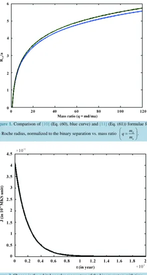
The simple form of Equation (60) is a reasonable approximation to the more accurate Eggleton [11] formula for mass ratios q0.9. Thus we see that the Roche lobe radius is directly proportional to the separation for a fixed mass ratio. Given Roche geometry and the structure of the star, we can now specify the mass transfer rate. In general, we expect the mass transfer to be a strong function of the “depth of contact”, defined as the amount by which the donor overflows its Roche lobe Rd =Rd−RL and of the structure of the star, which can be de-scribed in different ways depending on the problem at hand.
Figure 1. Comparison of [10] (Eq. (60), blue curve) and [11] (Eq. (61)) formulae for
the Roche radius, normalized to the binary separation vs. mass ratio d a m q
m
=
.
[image:12.595.168.459.169.404.2]Thus if d 0, 0 a
m
q a
m
= ≈ > which implies that the orbit will be enlarge and if d , 0 a
m
q a
m
= ≈ ∞ < that the
orbit will be shirk. This means the radius of a Roche lobe filling star depends only on the binary separation and the mass ratio. The blue curve shows that the stable conservative mass transfer while the green one is the unsta-ble mass transfer.
InFigure 2, we have plotted the equilibrium angular momentum values for a range of binary system with a time and for a mass ratio q = 1, taking the mass of the black hole MBH =1.75M. We here produce analytical solutions for the non conservative mass transfer in close binary system taking the initial masses of the primary and secondary as ma =2.5M and md =5M.
The change in mass for both the accretion and donor as well as the changing of the orbital angular frequency with time are derived in Equation (21) within the pre-assigned time scale of mass exchange as t=104 (years) and period p = 100 (days), the orbital angular momentum J continues to show a steady decreasing with the in-creasing time in Figure 3 and Figure 4.
Considering an interacting double degenerate system with initial masses of donor and accretor ma=0.24M and md =0.65M (dotted line) and a “semi-degenerate” low-mass helium star donor plus white dwarf accretor of the same initial masses (dash or blue line), and the periods (P = 2, 3, 4) from Roche lobe overflow; lower lim-its of the disk is equilibrium instability region according to [12] for q=0.5 and conventional evolutionary computations may be not adequate for description of mass transfer process.
From Equation (18), the change of orbital period is proportional to the change in Mdot. Prolonged, conserva-tive mass transfer is obtained when the initial mass of donor star is more massive, and the period decreases; hence star move close together.
4.2. The Binary Parameters
It is worthwhile to describe the binary parameters used by [4] [5] in their pioneering analysis in some detail, since we are using it as a comparison to our numerical solutions in Section (4.4). We shall thus obtain analytic as well as numerical solutions for a general polytropic index n to compare our results with those obtained from a full numerical evolution. The mass transfer rate for a polytropic donor is given by Jedrzejec (1969) assuming laminar flow, quoted by Paczynski & Sienkiewicz (1972) and from Equations. ((51)-(54)) we obtain:
3/ 2
0
n
d Ld
d
d
R R
m M
R
+
−
= −
[image:13.595.178.457.444.707.2] (69)
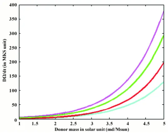
Figure 4. The total rate of change of the orbital angular frequency of the binary (Eq. (30)) related to the mass lost from the system of two point masses which will coalesce due to gravitational wave emission in a time interval shorter than 1010 yr, as a function of the donor mass in solar unit
(
md M)
. As we go from top to bottom on the right side; the lines (curves) are calculated for magenta (10M+10M(
BH+BH)
) which corresponds to an initial 1M donor whose central hydrogen abundance is 0.005 atthe onset of mass transfer, green (10M+1.4M
(
BH+NS)
) corresponds to a donor whose central hydrogen abundance has just reached zero at the onset of mass transfer, the red curve (line) is the analytical value of the rate of change of the orbital angular frequency versus donor mass in solar unit (the analytical value of those compact objects) and cyan (1.4M+1.4M(
NS+NS)
) corresponds to the case for which the donor has developed a 0.005M helium core.Raising both sides of the Equation (69) to the power 2 2
(
n+3)
and differentiating, we obtain:( )
2 2 3( )
2 2 3(
)
(
)
0 d
d
n
n d
d d Ld d Ld
d m
m M
t υ υ m ζ ζ
+
+
= − − + −
(70)
where we have set the factor RL Rd to unity, given that in most situations ∆Rd Rd. Defining a positive dimensionless mass transfer
(
0)
2 2( 3)n d
X = m M + , and a characteristic time scale 0
d
m M
τ = , Equation (70) becomes
3 2 d
d
n
d Ld
X
X t
ζ ζ τ
+
−
= − (71)
The solution can be easily inverted to yield
( )
( )
( )
(
)(
)
2 2 11 2
0 1 0 1 2
n n
d Ld
X t X X n ζ ζ t τ
− + +
= + + − (72)
where X
( )
0 is the initial mass transfer rate, normalized as Equation (72).Returning now to Equation (70), with the same definitions as Equation (72) for X and τ, we obtain for the general case in which driving is present
(
3 2 3 2)
d d
n n
d Ld
eq X
X X
t
ζ ζ τ
+ +
−
where 3 2
(
0)
(
)(
)
neq d d Ld d Ld
X + ≡ − m M = υ −υ τ ζ −ζ is the equilibrium value normalized to M0. Note that in the stable case, this value is positive; while it is negative in the unstable case. Before we attempt to solve the above differential equation, it is clear from its form and the signs just discussed, that it describes a stable solu-tion in which X →Xeq when q<qstable. if, however, q>qstable, the right had side of Equation (73) is positive even if the mass transfer vanishes initially, and it just gets bigger as the mass transfer grows. Since X diverges for the non driving case in a finite time, the driven case diverges even sooner.
Considering Equation (70) again we define
( )
2 2 3* n
d d eq
X m m
+
= , and
(
)
(
( )
)
2 2 3 *
1
n
d Ld md md eq
τ = υ −υ + . The differential equation for the evolution of mass transfer now becomes
( )
(
( )
)
* 3 2 * * * * d 1 1 d n XX X X
t τ
+
= − (74)
Thus, for the stable case (X*>0
, while (X*<0
for the unstable case, and τ*
is defined positive). The ge- neral analytic solution comprising both the stable and the unstable case can be given in terms of the hyper geo-metric function, as follows:
( )
3 2* * *
*
1 1
1, ; 1 ,
3 2 3 2
n d
t
X X X
n n τ + = + + +
(75)
Though it is not possible to invert this general solution to obtain the mass transfer rate X as a function of time, particular solutions for specific values of n can be inverted to obtain simple solutions. For example, n = 3/2 yields the [5] solution:
(
)
33 1
1 2 1 π
3 arctan
2 1 3 6
X t X X τ − + = − + − −
(76)
where, X = −
(
md µ)
1/3,(
)(
)
1/3 01 3 m md d Ld d Ld
τ = ζ −ζ υ −υ − . Likewise, n = 1/2 yields X*=tan
( )
t τ* , X*<0unstable and X* =tanh
( )
t τ* , X*>0stable.
4.3. Isothermal Atmospheres
In case of isothermal atmospheres, the mass transfer rate [13] [14] is given by
( ) ( ) 0e d d R L d
m = −m − α (77) where, α is the scale height. This form of the mass transfer equation is much simpler to integrate than the one for the polytropes considered above. With the same approximations and notation as in the steps leading to Equation (73), and defining 0 e(( ) )
d L R R d
X = −m m = − α , we obtain:
(
)
1 d d
d L d
eq R X X X X t ζ ζ τ α −
= − − (78)
This is easily integrable and invertible to get the following:
(
)
(
0)
1 1 e iso
eq
eq X X
X X τ τ
=
− − (79)
where τiso≡α Rd
(
υd −υL)
is the time scale required for the driving to change the depth of contact by ~α, and X0 is the initial value, always positive for physically meaningful cases. In the stable case Xeq >0, andeq
X →X , while Xeq <0 for the unstable case and X diverges in a finite time tdiv =τisoln 1
(
−Xeq X0)
. If no driving is present, we may set Xeq =0 and integrate Equation (78) for an isothermal donor.The result is again simple and instructive.
(
)
0 0 1 d d L X X R t X ζ ζ α τ =In the stable case, for any initial mass transfer, the system will detach and mass transfer will tend to zero. In the unstable case, any non-zero initial mass transfer will grow and diverge in a finite time.
We specify the parameters of the binary at its initial state; ma =0.62M, md =1.1M, Ra =0.012R, 0.0072
d
R = R, and a=0.037R and for the binary, it turns out that the adiabatic coefficients ζd ~ 0.54− and ~ 0.38
Ld
ζ − are related to Equations ((72), (73), (75), and (76)). We notice that since ζd > ζLd ; the ra- dius of the star increases at a rate faster than the Roche lobe radius, and the resulting mass transfer is unstable.
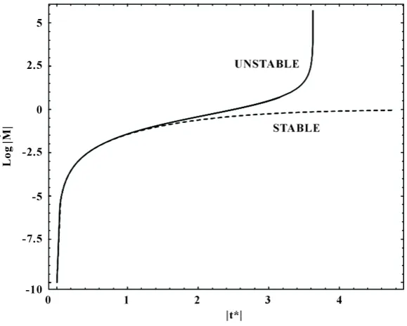
The analytic solutions, both the stable and the unstable, are shown in Figure 5.
Note that initially, the stable and the unstable solutions in Figure 5 almost exactly overlap. This is true as long as the system is either detached or the depth of contact is relatively small. As soon as the binary evolves to deeper contact, the unstable solution diverges rapidly and blows up in a finite time. This outcome is predicted by the unstable analytic solution which has been obtained by assuming that the basic primary parameters: the mass ratio q, driving rate υL and the masses of the components do not change during the evolution. This is obvious-ly not true, especialobvious-ly in the unstable case, since by definition in the unstable case these parameters are evolving rather rapidly (Figure 5).
4.4. Numerical Solutions
In Section (4.2 and 4.3), we have derived the basic evolution equations; Equations ((72), (73), (75), and (76)) from Equations ((51)-(54)) in Section (3.1) that for the numerical results and the corresponding analytic solu-tions for different cases, under certain restrictive approximasolu-tions. These analytic solusolu-tions are a useful reference to compare our numerical results to, since in the limit that the assumptions used to derive the analytic solution are met, the numerical solutions should approach the analytic ones. However, in general, the analytic solutions cannot explain the behavior of a given system accurately and especially when the system evolves rapidly, solv-ing the evolution equations numerically leads to a different outcome than what one would expect analytically.
Limitations of the Analytic Solutions
The analytic solutions of equations in Section (4.2 and 4.3) from Section (2.4) and through Section (3.1) are ob-tained under the following assumptions:
1) The driving rate given by υL is constant throughout the evolution.
[image:16.595.170.460.475.707.2]2) The separation “a” of the binary is effectively constant even though the mass transfer rate changes, which is not true for “a” “real system” (see Equation (36)).
3) The tidal effects are effectively ignored.
4) A system that is initially unstable (q>qstable), remains so throughout the evolution, since q is assumed to be the same throughout and it is possible for an initially unstable system to evolve to a stable configuration.
In order to overcome some of these shortcomings one has to numerically integrate the evolution equations in a self consistent way. In particular, in what follows, we allow for the changes in the masses of the components assuming conservative mass transfer (and hence the mass ratio q), allow the binary separation to change as a re-sult of any driving present, and compute the values of ζd and ζL as they evolve. The values of ζd depend on the adopted mass-radius relationship for the donor. To calculate ζL, we need to specify how the mass and angular momentum are redistributed in the binary during mass transfer which depends on the particular case at hand. For example, it depends on whether the stream impacts the accretor or if an accretion disk is present; if the mass transfer is sub-critical and conservative, or if mass and angular momentum are being ejected from the sys-tem following supercritical mass transfer (Figures 6-8).
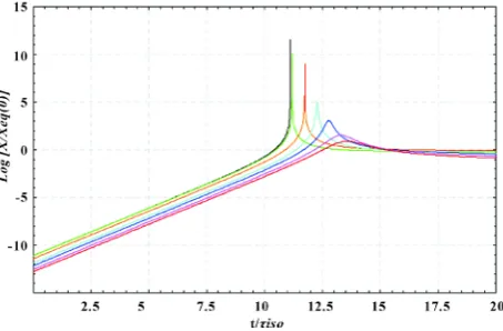
Figure 6. Numerical and Analytic Solutions for Polytropes. Comparison of numerical integrations with the analytic solution in Section (4.2). The mass transfer rate in solar mass normalized to the initial equilibrium rate as a function of time in units of the initial τ: analytic (red curve) and numerical- green (q = 0.985), blue (q = 0.875), magenta (q = 0.816), cyan (q = 0.656 same as [5]), Darkred (q = 0.625) and orange (q = 0.416).
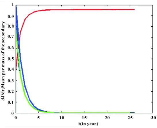
[image:17.595.204.428.242.417.2] [image:17.595.200.427.501.650.2]Figure 8. Loss of orbital angular momentum and decrease in the mass of the secondary with time (in year).
We simulate exactly the same initial conditions as the ones assumed to derive the analytic solution, a constant driving rate and the same mass-radius relationship. We then relax the constraints and let the system evolve in a self-consistent manner for different values of the mass ratio q. We observe that initially all the curves overlap, but as the depth of contact increases, the mass transfer rate increases. As the system evolves, the orbital separa-tion, which is decreasing initially, begins to increase as per Equation (36) which in turn decreases the driving rate. At some point during the evolution q becomes less than qstable and the system evolves to stable mass transfer rates. From our analysis in Section (4.2), we expect the systems with q>qstable to be unstable, and the higher the mass ratio, the more unstable the system is. This is indeed what we observe in the numerical solutions. The numerical solutions reach a peak in the mass transfer rate in a finite time, but turn around and a stable mass transfer is established. In any case, our results suggest and demonstrate that at least some of the binaries that start off unstable do survive the mass transfer instability and evolve into systems like AM CVn—evolving to higher separations and diminishing mass transfer rates. This result, which is not predicted by the analytic solu-tion, has important consequences for population synthesis, understanding AM CVn type systems.
In Figure 7, we plot the analytic and numerical solutions for an isothermal donor for different values of the mass ratio. Unlike the polytropic donor case, which has a fixed reference point where the donor fills its Roche lobe (Rd =RL), the isothermal case does not have a fixed reference point to which we can normalize our results. We, rather arbitrarily start the integrations when the depth of contact is Rd −RL = −11.5α, corresponding to an initial mass transfer rate of 10−5 of the reference rate. The behavior of the systems is qualitatively the same as the polytropic donors. Note that the y-axis in Figure 7 is the natural logarithm of x which from Section (4.3), is just the depth of contact Rd −RL in units of the pressure scale height α, normalized to the reference depth cor-responding to the equilibrium rate for q = 0.663.
Thus we here produce a numerical analysis for the rate of change of orbital angular momentum(green line), the rate of change of mass of the secondary star (blue line), and Increase in the mass of the primary with time (in year) in a close binary system taking the initial masses of the primary as ma =2.5M and md =5M. For the present calculation, we consider the values of the parameters as a=2.78, p = 30 (per year) and q = 0.8. But af-terwards as the mass accretion rate by the primary varies slowly and consequently ma shows a very weak vari-ation with time, the orbital angular momentum Jorb continues to slow as steady decreasing with the decreasing in md .
5. Conclusions
binary star systems in which we track the mass of each component, the total mass of the system, the orbital an-gular momentum and the spin anan-gular momenta of each component. We have included the effects of mass and angular momentum loss from the system and also the exchange of mass and angular momentum between the components of the binary.
The main reason why many binary systems transfer matter at some stage of their evolutionary lifetimes is during the system evolution. One of the stars in a binary system may increase in radius filling its Roche lobe, or the binary separation may shrink because orbital angular momentum is being lost from the system as a conse-quence of stellar wind mass loss, or gravitational radiation.
There are two general mechanisms for the transferring angular momentum out of the system: First, binary systems emit gravitational radiation, which carries away angular momentum. The rate of angular momentum loss increases as the orbital separation decreases, but it decreases as the total mass of the system decreases. Because both the secondary mass and the orbital separation decrease as CV systems evolving, the net effect is a loss mechanism that does not depend strongly on the orbital period.
Our investigation indicates that the stability of the mass transfer processes depends on: how the radius of the donor star responds to the mass loss, how the orbit responds to mass transfer, and how the mass-gainer responds to the matter that is being dumped on it.
The Roche lobe of the mass donor shrinks as a consequence of its mass loss, increasing the rate at which it loses mass is referred to unstable mass transfer and the Roche lobe of the mass donor grows as a consequence of its mass loss, stopping the mass transfer is referred to stable mass transfer.
In this paper we have made an effort to find a numerical and analytical solutions for conservative and non-conservative mass transfer in close binary systems which can address the gradually reducing rate of the mass accretion by the accretor from the donor with respect to time as well as with respect to the increase in mass of the accretor [15]. In view of this we have presented the time dependent profiles of the masses of both the component stars in a close binary as well as the orbital angular momentum of the system. Our analytical solu-tions shows for the non-conservative mass transfer in close binary system taking the initial masses of the prima-ry and secondaprima-ry as ma =2.5M and md =5M with 4
10
t= (in years) and p = 100 (in days), and
(
)
10M+10M BH+BH which corresponds to an initial 1M donor whose central hydrogen abundance is 0.005 at the onset of mass transfer, 10M+1.4M
(
BH+NS)
corresponds to a donor whose central hydro-gen abundance has just reached zero at the onset of mass transfer and 1.4M+1.4M(
NS+NS)
corres-ponds to the case for which the donor has developed a 0.005M helium core (see Figure 4), the orbital an-gular momentum J continues to show a steady decreasing with the increasing time (see Figure 2).In conservative mass transfer and from Equation (15); if ma is the mass losing star, ma will be negative, therefore we conclude that if the mass donor star is more massive, then the orbit will shrink and hence period decreases. But if the mass donor is less massive than the accretor component then orbit will be widened and pe-riod increases.
We have also presented a new finding (analytic and numeric solutions) for the evolution of binary systems, generalizing the results of [4] to binaries with any polytropic index and to binaries with isothermal atmospheres. The analytic solutions always predict that if a binary attains contact when the mass ratio q is such that the en-suing mass transfer is unstable, the binary merges in a finite time. On the other hand, the numerical solutions predict that a binary that undergoes unstable mass transfer at initial contact can evolve to a state of stable mass transfer, survive and evolve into an AM CVn type system. Moreover, the analytic solutions also discussed here assume that the driving rates υd and υL in Equation (70) remain constant while the depth of contact changes. This is only approximately true; and a self-consistent solution will require numerical integrations. This is a situ-ation we encounter in some large-scale hydrodynamic simulsitu-ations of mass transfer in poly tropic binaries. We note that from Equations ((54), and (72)) in the stable case, ζd >ζL
(
q<qstable)
, the mass transfer decays asymptotically to zero over a characteristic time τchr τ(
n 1 2) ( )
y 0 n 1 2(
ζd ζL)
+
= + − , it will blow up in finite time equal to τchr. Thus, the essence of the stability of mass transfer in a binary is already contained in the sim-ple case of no driving. The presence of driving exacerbates the natural instability or, in the stable case, it settles asymptotically to a non-zero stable mass transfer, which we have been observed in AM CVns, CVs and LMXBs. In our study numerical solutions indicates more physical descriptions than analytical (Figures 1-5) one as shown in Figures 6-8.
every binary in which mass is transferred from the less massive star is stable on both dynamical and thermal time scales. If the mass donor has a radiative envelope (not treated here), it will shrink in response to mass loss, and lose mass stable. If the donor has a convective envelope, a modestly sized core will stabilize it sufficiently to prevent mass loss on the dynamical time scale.
Acknowledgements
We thank Entoto Observatory and Research Center for supporting this research. Negu, thanks Jigjiga University for giving study leave. This research has made use of NASA’s Astrophysical Data System.
References
[1] Shore, S.N. (1994)Observations and Physical Processes in Interacting Binaries. Springer, Berlin Heidelberg, 1-133.
http://dx.doi.org/10.1007/3-540-31626-4_1
[2] Soberman, G.E., Phinney, E.S. and van den Heuvel, E.P.J. (1997) Stability Criteria for Mass Transfer in Binary Stellar Evolution. Astronomy and Astrophysics, 327, 620-635.
[3] Konstantin, A.P. (2014) The Evolution of Compact Binary Star Systems. Living Reviews in Relativity, 17, 3.
[4] Pennington, R.(1985) Interacting Binary Stars. Pringle, J.E. and Wade, R.A., Eds., Cambridge Astrophysics Series, Cambridge University Press, Cambridge, 197-199.
[5] Hjellming, M.S. and Webbink, R.F. (1987)Thresholds for rapid mass transfer in binary systems. I—Polytropic Models. The Astrophysical Journal, 318, 794-808. http://dx.doi.org/10.1086/165412
[6] Ruderman, M., Shaham, J. and Tavani, M. (1989) Accretion Powered by Compact Binaries. The Astrophysical Journal, 3, 507.
[7] Tessema, S.B. (2014) Stability of Accretion Discs around Magnetized Stars. International Journal of Astronomy and Astrophysics, 4, 319-331. http://dx.doi.org/10.4236/ijaa.2014.42026
[8] Lightman, A.P. and Eardley, D.M. (1974) Black Holes in Binary Systems: Instability of Disc Accretion. The Astrophy- sical Journal, 187, L1.
[9] Gharami, P., Ghosh, K. and Rahaman, F. (2014) A Theoretical Model of Non-Conservative Mass Transfer with Non- Uniform Mass Accretion Rate in Close Binary Stars.General Relativity and Quantum Cosmology, 366, 1511.
[10] Plavec, A. and Paczynski, B. (1971) Numerical Simulations of Dynamical Mass Transfer in Binaries. Annual Review of Astronomy and Astrophysics, 9, 183.
[11] Lajoie, C.-P. and Sills, A. (2010) Mass Transfer in Binary Stars Using Smoothed Particle hydrodynamics. II. Eccentric Binaries. The Astrophysical Journal, 726, 13 p.
[12] Tsugawa, M. and Osaki, Y. (1997) Disk Instability Model for the AM Canum Venaticorum Stars. PASJ: Publ. Astron. Soc. Japan, Vol. 49, 75-84.
[13] Paczynski, B. and Sienkiewicz, R. (1972) Mass Transfer Effects in Binary Star Evolution. Acta Astronautica, 22, 73.
[14] Vayujeet, G. (2007) Mass Transfer and Evolution of Compact Binary Stars. Astronomy & Astrophysics, 202, 93.