Modeling and Design of Real Time Pricing Systems Based on Markov Decision Processes

(1)

http://dx.doi.org/10.4236/am.2014.510141

How to cite this paper: Kobayashi, K., et al. (2014) Modeling and Design of Real-Time Pricing Systems Based on Markov De-cision Processes. Applied Mathematics, 5, 1485-1495. http://dx.doi.org/10.4236/am.2014.510141

Modeling and Design of Real-Time Pricing

Systems Based on Markov Decision

Processes

Koichi Kobayashi

1*

, Ichiro Maruta

2

, Kazunori Sakurama

3

, Shun-ichi Azuma

2

1_{School of Information Science, Japan Advanced Institute of Science and Technology, Ishikawa, Japan} 2_{Graduate School of Informatics, Kyoto University, Kyoto, Japan}

3_{Graduate School of Engineering, Tottori University, Tottori, Japan} Email: *_{[email protected]}

Received 2 April 2014; revised 2 May 2014; accepted 9 May 2014

This work is licensed under the Creative Commons Attribution International License (CC BY). http://creativecommons.org/licenses/by/4.0/

Abstract

A real-time pricing system of electricity is a system that charges different electricity prices for dif-ferent hours of the day and for difdif-ferent days, and is effective for reducing the peak and flattening the load curve. In this paper, using a Markov decision process (MDP), we propose a modeling me-thod and an optimal control meme-thod for real-time pricing systems. First, the outline of real-time pricing systems is explained. Next, a model of a set of customers is derived as a multi-agent MDP. Furthermore, the optimal control problem is formulated, and is reduced to a quadratic program-ming problem. Finally, a numerical simulation is presented.

Keywords

Markov Decision Process, Optimal Control, Real-Time Pricing System

1. Introduction

In recent years, there has been growing interest in energy and the environment. For problems on energy and the environment such as energy saving, several approaches have been studied (see, e.g., [1] [2]). In this paper, we focus on real-time pricing systems of electricity. A real-time pricing system of electricity is a system that charges different electricity prices for different hours of the day and for different days, and is effective for reducing the peak and flattening the load curve (see, e.g., [3]-[6]). In general, a real-time pricing system consists of one controller deciding the price at each time and multiple electric customers such as commercial facilities

(2)

and homes. If electricity conservation is needed, then the price is set to a high value. Since the economic load becomes high, customers conserve electricity. Thus, electricity conservation is achieved. In the existing methods, the price at each time is given by a simple function with respect to power consumptions and voltage deviations and so on (see, e.g., [6]). In order to realize more precisely pricing, it is necessary to use a mathematical model of customers.

In this paper, using a Markov decision process (MDP), we propose a mathematical model of real-time pricing systems. Since in many cases, the status of electricity conservation of customers is discrete and stochastic, it is appropriate to use an MDP. Then, a set of electricity customers is modeled by a multi-agent MDP. Furthermore, we consider the finite-time optimal control problem. By appropriately setting the cost function, it is achieved that customers conserve electricity actively. This problem can be used for the model predictive control method, which is a control method that the finite-time optimal control problem is solved at each time. In addition, the finite-time optimal control problem can be reduced to a quadratic programming problem. The proposed approa- ch provides us with a basic of real-time pricing systems.

This paper is organized as follows. In Section 2, the outline of real-time pricing systems is explained. In Section 3, a model of electricity customers is derived. In Section 4, the optimal control problem is formulated, and its solution method is derived. In Section 5, a numerical simulation is shown. In Section 6, we conclude this paper.

Notation: Let  denote the set of real numbers. Let I_n, 0m n× denote the n n× identity matrix, the m n× zero matrix, respectively. For simplicity, we sometimes use the symbol 0 instead of 0m n× , and the symbol I instead of I_n. For two events A B, , let E A B_ _ denote the conditional expected value of A under the event B.

2. Outline of Real-Time Pricing Systems

[image:2.595.161.468.531.702.2]

In this section, we explain the outline of real-time pricing systems studied in this paper.

Figure 1shows an illustration of real-time pricing systems studied in this paper. This system consists of one controller and multiple electric customers such as commercial facilities and homes. For an electric customer, we suppose that each customer can monitor the status of electricity conservation of other customers. In other words, the status of some customer affects that of other customers. For example, in commercial facilities, we suppose that the status of rival commercial facilities can be checked by lighting, Blog, Twitter, and so on. Depending on power consumption, i.e., the status of electricity conservation, the controller determines the price at each time. If electricity conservation is needed, then the price is set to a high value. Since the economic load becomes high, customers conserve electricity. Thus, electricity conservation is achieved.

In this paper, the status of electricity conservation of each customer is modeled by a Markov decision process (MDP). Then a set of customers is modeled by a multi-agent MDP (MA-MDP). Furthermore, by using the obtained MA-MDP model, we consider the optimal control problem and its solution method.

(3)

3. Model of Customers

First, consider modeling the dynamics of each customer by a one-dimensional MDP. The value of the state x is randomly chosen among the finite set

{

0,1,,n−1

}

. The element of

{

0,1,,n−1

}

expresses the status of electricity conservation, and “0” implies the status that a customer conserves electricity maximally, “n−1” implies the status that a customer does not conserve electricity. Then the MDP of a customer is given by

(

t 1

)

P u t

(

( )

)

( )

t

π + = π (1)

where u t

( )

∈ is the control input, and corresponds to the price. The vector

( )

( ) ( )

( )

T

[ ]

0 1 1 0,1

n n

t t t t

π =π π π −  ∈ denotes the probability distribution, that is,

π

i

( )

t ∈

[ ]

0,1 implies the probability that the state is i at time t. In addition, the initial probability distribution must satisfy the following condition:

( )

1 0 0 1. n i i π − = =

∑

The transition probability matrix P u t

(

( )

)

is given by

( )

(

)

( )

11 1 1 1

21 2 2 2

1

.

n

n n nn n

a b u t a b u t

P u t

a b u t a b u t

 + +   ₊ ₊    =     + +          

The control input is determined under the condition for each element:

( )

0≤aij+b u ti ≤1 (2) and the condition for each column:

( )

1 1. n ij i i

a b u t

=

+ =

∑

(3)

Next, consider modeling the dynamics of a set of customers by an MA-MDP. The number of customers is given by q. For the customer i, the state is given by i

{

0,1, , 1

}

x ∈  n− , and from (1), the MDP model is given by

(

1

)

(

( )

)

( )

.

i i i i

t P u t t

π + = π

Then, we suppose that the MA-MDP model expressing the dynamics of a set of customers is given by

(

)

(

)

(

)

( )

(

)

( )

(

)

( )

(

)

( )

1 1

1 11 12 1 1

2 2

21 22 2

1 2 1 1 , 1 q q q q q q

q q qq

P u t I I

t t

I P u t I

t t

t _I _I _P _u _t t

λ λ λ

π π

λ λ λ

π π

π _λ _λ _λ π

   +  _ _   ₊  _ _   ₌_ _    _ _    _ _  +       _ _     _ _ _ _   (4)

where λ_ij expresses the effect of couplings between customers, and is a constant satisfying the following condition:

1

1, 1, 2, , . q ij j i q λ = = =

∑

 (5)

(4)

4. Optimal Control

4.1. Problem Formulation

Consider the following problem.

Problem 1. Suppose that for the MA-MDP model (4) expressing the dynamics of customers, the initial state

( )

0 0

i i

x =x , i=1, 2,,q, the desired state x_d, and the prediction horizon N are given. Then, find a control input sequence u ti

( )

, i=1, 2,,q, t=0,1,,N−1 minimizing the following cost function

( )

(

)

2

(

( )

)

2

( )

0 0 1

0

q N

i i i i

i d i

t i

J E Q x t x R u t x x

= =

 

= _ − + = _

 

∑∑

(6)

subject to the following constraint:

( ) ( )

( )

(

1 2

)

, , , q ,

f u t u t  u t ≤M (7)

where f

( )

⋅ is a given linear function, M is a given vector. Q Ri, i are given weights.

Hereafter, for simplicity of notation, the condition xi

( )

0 =x₀i in the cost function (6) is omitted.

By using the constraint (7), the input constraint such as u_min≤u ti

( )

≤u_max can be imposed. In addition, by adjusting Q Ri, i, several specifications such that the state

( )

i

x t must converges to the neighborhood of the desired state x_d can be considered.

4.2. Solution Method

We derive a solution method for Problem 1. First, consider the MDP model (1). The MDP model is a class of nonlinear systems. However, in this case, it can be transformed into a linear system. The MDP model (1) can be rewritten as

(

)

( )

( ) ( )

(

( )

)

( ) ( )

(

( )

)

( ) ( )

(

( )

)

1 1 2 1 1 1 , n n n n

b u t t t

t A t

b u t t t

π π π π π π π π  + +    + +   + = _{+ } _    _{+ +}        where

11 12 1

21 22 2

1 2

.

n

n n nn

a a a

A

a a a

      =             

By the property of the probability distribution, the relation

π

₁

( )

t + +

π

_n

( )

t =1 holds. From this fact, the MDP model (1) can be equivalently transformed into the following linear system:

( )

t 1 A

( )

t Bu t

( )

,

π

+ =

π

+ (8)

where B=

[

b b₁ ₂  b_n

]

T.

Next, by using the linear system (8), consider representing the MA-MDP model (4) as a linear system. The linear system for the customer i is denoted by

(

1

)

( )

.

i i i i i

t A t B u t

π + = π +

Then, the MA-MDP model (4) can be equivalently transformed into the following linear system:

(

)

(

)

( )

1 1 1

1

, 1

q q q

t t u t

A B

t t u t

π π π π  +       ₌  ₊          ₊           

(5)

where

1 1

11 1 11

1 0 , . 0 q q q

q qq qq

A I B

A B

I A B

λ λ λ

        =_ _ =_ _              

Finally, consider the cost function (6). Define

[

]

1: 0 1 1 ,

L =  n−

(

)

2

2 2

2: 0 1 1 .

L =_  n− _

Then we can obtain

( )

1

( )

,

i i

E x t_  =_ Lπ t

( )

(

)

2

( )

2 .

i i

E_ x t  =_ Lπ t

 

Therefore, the cost function (6) can be rewritten as

( )

(

)

(

( )

)

( )

(

)

( )

(

( )

)

(

) ( )

(

( )

)

2 2 0 1

2 ₂ 2

0 1 2 ₂ 2 1 0 1 2 2 . q N i i

i d i

t i

q N

i i i

i i d i d i

t i

q N

i i

i d i i d

t i

J E Q x t x R u t

Q E x t Q x E x t Q x R u t

Q L x L π t R u t Q x

= = = = = =   = _ − _+     _ _ = _ _− _ _+ +   = − + +

∑∑

(10)

From the above discussion, Problem 1 is equivalent to the following problem.

Problem 2

( )

( ) ( )

( )

find , 1, 2, ,

0,1, , 1,

min Cost function 10 ,

subject to System 9 ,

Inequality constraint 2 , 7 ,

Equality constraint 3 .

i

u t i q

t N

=

= −

 

Problem 2 is reduced to a quadratic programming (QP) problem, and can be solved by a suitable solver such as MATLAB and IBM ILOG CPLEX. In addition, if Ri=0, then Problem 2 is reduced to a linear programming (LP) problem (we remark that Q xi 2d in the cost function (10) is a constant). See [7] for further details.

5. Numerical Example

Since it is difficult to use data in real systems, we present an artificial example. The state is chosen among the

finite set

{

0,1, 2,3

}

. The number of consumers is given by q=5. The coefficient matrices A Bi, i in the linear system for the consumer i are given by

1 2 3

0.3 0.4 0.3 0.5 0.5 0.6 0.5 0.3 0.6 0.3 0.1 0.3

0.4 0.3 0.2 0.2 0.2 0.2 0.1 0.4 0.1 0.3 0.4 0.2

, , ,

0.2 0.2 0.2 0.2 0.2 0 0.2 0.3 0.2 0.3 0.4 0.1

0.1 0.1 0.3 0.1 0.1 0.2 0.2 0 0.1 0.1 0.1 0.4

A A A

(6)

4 5

0.7 0.5 0.4 0.5 0.3 0.5 0.2 0.4 0.6

0.1 0.2 0.1 0.2 0.1 0.2 0.3 0.4 0.2

, , .

0.1 0.1 0.1 0.2 0.3 0 0.3 0.1 0.2

0.1 0.2 0.4 0.1 0.3 0.3 0.2 0.1 0.2

i

A A B

     

    ₋ 

     

= = =

    − 

    ₋ 

     

The parameters λ_ij in (9) are given by

11 12 13 14 15

21 22 23 24 25

31 32 33 34 35

41 42 43 44 45

51 52 53 54 55

0.7 0.3 0 0 0

0.2 0.6 0.2 0 0

. 0 0.1 0.8 0.1 0

0 0 0.2 0.7 0.1

0 0 0 0.1 0.9

λ λ λ λ λ λ λ λ λ λ λ λ λ λ λ λ λ λ λ λ λ λ λ λ λ

   

   

  = 

   

  _ _

 

The parameters N, x_d, Q_i, and R_i are given by N =10, xd =0, Qi=1, and Ri =0, respectively. From Ri=0, Problem 2 is reduced to an LP problem. The initial state is given by

( )

[

]

T

0 0 0 0 1

i

x = . In

addition, the input constraint 0 i

( )

1 u t

≤ ≤ is imposed.

In this numerical example, we consider the following two cases:

• The price for each customer is the same (i.e., u t1

( )

=u2

( )

t ==uq

( )

t holds). • The price for each customer is different.

Case (i) is the conventional case in real-time pricing systems. In Case (ii), we suppose that the difference in the price is covered by using local concurrencies such as the Eco-point point system [8]. The Eco-money system

[9] in Japan were introduced to stimulate the economy and raise awareness of global warming. In the Eco-point point system, many points, which correspond to money in a local concurrency, are given for the products that are effective from the viewpoints of electricity conservation and the environment. Such a system for energy management systems has been discussed in [10].

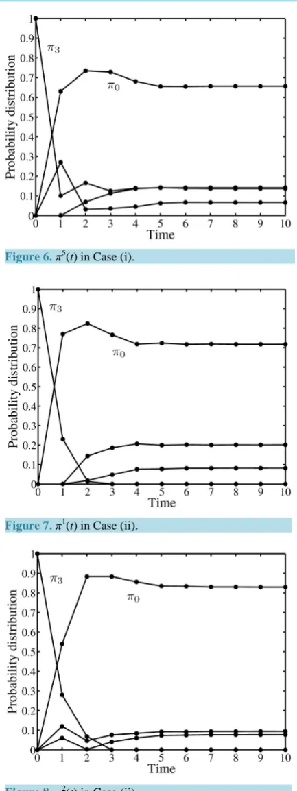
Next, we present the computational results. First, the computational result in Case (i) is explained. Figures 2-6 show the probability distribution for each customer. From these figures, we see that π₀i

( )

t increases and

( )

3

i t

π decreases. Thus, the state converges to 0, which corresponds to the status that a customer conserves electricity maximally, with a certain probability. Furthermore, the optimal value of the cost function is 97.5902, and the optimal control input is derived as

( )

0 0.5, 1

( )

0.65, 2

( )

0.6637, 3

( )

0.5664, 4

( )

0.5168,

u = u = u = u = u =

( )

5 0.5151,

( )

6 0.5184,

( )

7 0.5189,

( )

8 0.5192,

( )

9 0.5192.

u = u = u = u = u =

(7)

Figure 3. π2(t) in Case (i).

Next, the computational result in Case (ii) is explained. Figures 7-11 show the probability distribution for

(8)

Figure 7. π1(t) in Case (ii).

Figure 6and Figure 11). Furthermore, the optimal value of the cost function is 84.5057, and we see that the optimal value of the cost function is improved. The optimal control input

( )

₁

( ) ( ) ( ) ( ) ( )

₂ ₃ ₄ ₅ T

[image:8.595.205.422.77.655.2]

(9)

( )

1 1 0.6637 0.5478 0.5755

1 1 0.6792 0.5942 0.5719

0 0.5 , 1 0.8575 , 2 0.6081 , 3 0.5492 , 4 0.5086

1 0.615 0.5664 0.5135 0.52

0.5 0.785 0.7622 0.7790

u u u u u

       

       

= = = = =

       

       

,

79

0.7627

 

 

 

( )

0.5755 0.5811 0.5811 0.5817

0.5825 0.5831 0.5850 0.5850

5 0.5068 , 6 0.5057 , 7 0.5048 , 8 0.5045

0.5473 0.5576 0.5608 0.5625

0.7752 0.7669 0.7726 0.7684

u u u u

       

       

      

= = = =

      

       

( )

0.5816

0.5853

, 9 0.5043 .

0.5629

0.7713

u

 

 

  

 = 

  

 _ _

From these values, we see that in the steady state, u5

( )

t is widely different to u ti

( )

, i=1, 2, 3, 4. Thus, in the system considered here, it is appropriate to use a local concurrency.

6. Conclusions

(10)

stochastic, and the use of the MDP model is effective. A real-time pricing system is modeled by multi-agent MDPs, and the optimal control problem is reduced to a QP problem. Furthermore, a numerical simulation has been shown. The proposed method provides us with a new method in real-time pricing of electricity.

There are several open problems. First, it is important to develop the identification method of the MA-MDP model based on the existing result (see, e.g., [11]) for MDPs. Since the effect of couplings between customers was simplified, it is also important to consider modeling it more precisely. Next, the optimal control problem is reduced to a QP problem or an LP problem. These problems can be solved faster than a combinatorial optimization problem such as a mixed integer programming problem. However, for large-scale systems, the computation time for solving the optimal control problem will be long. Then, it is important to develop a distributed algorithm.

Acknowledgements

This research was partly supported by JST, CREST.

References

[1] Camacho, E.F., Samad, T., Garcia-Sanz, M. and Hiskens, I. (2011) Control for Renewable Energy and Smart Grids. In: Samad, T. and Annaswamy, A.M., Eds., The Impacy of Control Technology, IEEE Control Systems Society, New York.

[2] Ruihua, Z., Yumei, D. and Yuhong, L. (2010) New Challenges to Power System Planning and Operation of Smart Grid Development in China. Proceedings of the 2010 International Conference on Power System Technology, Hangzhou, 24-28 October 2010, 1-8.

[3] Borenstein, S., Jaske, M. and Rosenfeld, A. (2002) Dynamic Pricing, Advanced Metering, and Demand Response in Electricity Markets. Center for the Study of Energy Markets, University of California, Berkeley.

[4] Roozbehani, M., Dahleh, M. and Mitter, S. (2010) On the Stability of Wholesale Electricity Markets under Real-Time Pricing. Proceedings of the 49th IEEE Conference on Decision and Control, Atlanta, 15-17 December 2010, 1911- 1918.

[5] Samadi, P., Mohsenian-Rad, A.-H., Schober, R., Wong, V.W.S. and Jatskevich, J. (2010) Optimal Real-Time Pricing Algorithm Based on Utility Maximization for Smart Grid. Proceedings of the 1st IEEE International Conference on Smart Grid Communications, Gaithersburg, 4-6 October 2010, 415-420.

[6] Vivekananthan, C., Mishra, Y. and Ledwich, G. (2013) A Novel Real Time Pricing Scheme for Demand Response in Residential Distribution Systems. Proceedings of the 38th Annual Conference of the IEEE Industrial Electronics So-ciety,Monteral, 25-28 October 2012, 1954-1959.

[7] Bello, D. and Riano, G. (2006) Linear Programming Solvers for Markov Decision Processes. Proceedings of the 2006

IEEE Systems and Information Engineering Design Symposium, Charlottesville, 28 April 2006, 90-95.

http://dx.doi.org/10.1109/SIEDS.2006.278719

(11)

[9] Kyoto Eco Money. http://www.city.kyoto.jp/koho/eng/topics/2012_8/index.html

[10] Sawashima, K., Kubota, Y., Lu, H., Takemae, T., Yoshida, K. and Wan, Y. (2011) Socio-Personal Energy Manage-ment System. Keio ALPS2011 Group K Final Report.

http://lab.sdm.keio.ac.jp/alps2011k/FinalReport-ALPS2011-K.pdf