An Improved Decision based Asymmetric Trimmed Median Filter for Removal of High Density Salt and Pepper Noise

An Improved Decision based Asymmetric Trimmed

Median Filter for Removal of High Density Salt and

Pepper Noise

Abhishek Kesharwani

Sumit Agrawal Mukesh Kumar Dhariwal

CSE DEPT, UIT RGPV BHOPAL CSE DEPT, SATI VIDISHA CSE DEPT, UIT RGPV BHOPAL

ABSTRACT

An improved decision based asymmetric trimmed median filter (IDBATMF) algorithm for the restoration of gray scale, and color images that are highly corrupted by salt and pepper noise (SPN) is proposed in this paper. The proposed algorithm selects a 3 × 3window around pixel being processed. If the selected window consists of 0’s, 255’s and other random values, then the noisy pixel is replaced with the trimmed median value of the elements in selected window. When all the pixel values are 0’s and 255’s then the decision is taken based on numbers of 0 and 255 values in the window. If 6 or more pixels are 0 (or 255) then the pixel being processed is replaced with 0 (or 255), else it is replaced with mean of value of all the elements present in the selected window. Setting the pixel as 0 or 255 ensures that a large black or white patch of the image is restored satisfactorily. The proposed algorithm shows better results than existing median filters including the recent Modified Decision Based Unsymmetrical Trimmed Median Filter (MDBUTMF). Experimental results show improvements both visually and quantitatively compared to that of the MDBUTMF and other standard filters.

Keywords

Impulse noise, salt and pepper noise, Image de-noising, Median filter, asymmetric trimmed median filter, Decision based filter.

1.

INTRODUCTION

Impulse noise is a special type of noise which can have many different origins. Images are often corrupted by impulse noise caused by malfunctioning of camera’s sensor cells, transmission errors, faulty memory locations or timing errors in analog-to-digital conversion. Salt and pepper noise (SPN) is a type of impulse noise which can corrupt the image, where the noisy pixels can take only the maximum and minimum values in the dynamic range. Since, linear filtering techniques are not effective in removing impulse noise, non-linear filtering techniques are widely used in the restoration process. The standard median filter (MF) [1] has been established as reliable method to remove SPN without damaging the edge details. However, the major drawback of MF is that, the filter is effective only for low noise densities, and additionally, exhibits blurring if the window size is large and leads to insufficient noise suppression if the window size is small [2]. When the noise level is over 50% the edge details of the original image will not be preserved by MF. Adaptive Median Filter (AMF) [3] also performs well at low noise densities. But at high noise densities the window size has to be increased which may lead to blurring of image. In switching median filter [4], [5] the decision is based on a pre-defined threshold value. The major drawback of this method is that defining a robust decision is difficult. Also these filters will not take into account the local features as a result of which

details and edges may not be recovered satisfactorily, especially when the noise level is high.

To overcome the above drawback, Decision Based Algorithm (DBA) is proposed [6]. In DBA, the image is denoised by using a 3 × 3 window. If the processing pixel value is 0 or 255 it is processed, else it is left unchanged. At high noise density the median value will be 0 or 255 which again is noisy. In such case, neighboring pixel is used for replacement. This repeated replacement of neighboring pixel produces streaking effect [7]. In order to avoid this drawback, Decision Based Unsymmetric Trimmed Median Filter (DBUTMF) is proposed [8]. At high noise densities, if the selected window contains all 0’s or 255’s or both then, trimmed median value cannot be obtained. So this algorithm does not give better results at very high noise density. This issue is addressed in Modified Decision Based Unsymmetric Trimmed Median Filter (MDBUTMF) algorithm [9].

In MDBUTMF if all the pixels in a 3 × 3 window are 0 or 255, then processing pixel is replaced with mean of the elements in selected window. But MDBUTMF suffers from another issue, it assumes that the all the pixel with 0 or 255 value are noisy and the de-noised images should not have any pixels with extreme gray-level values. Though this is the working principle for the algorithm, but may not always be correct. It is possible to have certain patches in an image which are actually white (may be some background in a landscape image) or black (may be photo taken in night). In such cases the image restoration process should be able to identify the regional feature in the image and correct it accordingly. The proposed Improved Decision Based Asymmetric Trimmed Median Filter (IDBATMF) algorithm removes this drawback and gives better results in such white or black patches of the image as well.

The rest of the paper is structured as follows. A brief Literature Survey is presented in Section 2. Section 3 describes the Proposed Algorithm. Section 4 presents the Illustration of proposed algorithm with examples. The simulation results for various images and a comparative performance of algorithm is given in Section 5. Section 6 draws the conclusion of the proposed work.

2.

LITERATURE SURVEY

2.1

Impulse Noise Model

Impulse noise corruption is extremely common in digital pictures. Impulse noise is often freelance and unrelated to the image pixels and is haphazardly distributed over the image. thus not like mathematician noise, for AN impulse noise corrupted image all the image pixels are not noisy, variety of image pixels are noisy and also the remainder of pixels are noise free. Impulse noise is more classified as salt and pepper style of noise and random valued impulse noise.

-0) and it seems as black and white spots on the pictures. If p is that the total noise density then salt noise and pepper noise can have a noise density of p/2.This can be mathematically delineate as below.

(1)

Where Yi,j represents the noisy image pixel, p is the total

noise density of impulse noise and Yi,j is the uncorrupted

image pixel. At times the salt noise and pepper noise may have different noise densities p1 and p2 and the total noise density will be p = p1 + p2.

In case of random valued impulse noise, noise will take any gray level value from 0 to 225. during this case conjointly noise is at random distributed over the complete image and probability of prevalence of any gray level value as noise will be same. we can mathematically represent random valued impulse noise as below.

(2)

Where ni,j is the gray level value of the noisy pixel.

2.2

Linear Filters

Filtering [1] is a technique for modifying or enhancing an image. as an example, you can filter an image to emphasise certain features or take away alternative features. Mathematically, a filter could also be outlined as a perform that maps an image x into image y:

(3)

When the function F satisfies each the superposition and proportionality principles, the filter is said to be linear. Two-dimensional and m-Two-dimensional linear filtering is concerned with the extension of one-dimensional filtering techniques to two and more dimensions. If impulse response of a filter has solely finite number of non-zero values, the filter is named a finite impulse response (FIR) filter. Otherwise, it's an infinite impulse response (IIR) filter. If the filter evaluates the output image only with the input image, the filter is named non-recursive. On the opposite hand, if the analysis method requires input image samples in conjunction with output image samples, it's referred to as recursive filter.

2.3

Median Filters

Median Filters [1] are very effective in removing impulse noise at low density levels. The median filter follows the moving window principle for filtering. A 3 × 3, 5 × 5 or 7 × 7 kernel of pixels is scanned over pixel matrix of the complete image. The median of the pixel values within the window is computed, and therefore the center pixel of the window is replaced with the computed median. Median filtering is completed by, initial sorting all the pixel values from the surrounding neighborhood into numerical order so substitution the pixel being considered with the center pixel value. Note that the median value must be written to a separate array or buffer in order that the results are not corrupted because the method is performed.

2.4

‘α’ Trimmed Mean Filter

‘α’ trimmed Mean Filter (ATMF) [1] is a Non Linear filter that's used to remove the impulse noise employing a parameter known as ‘α’. The parameter ‘α’ refers to trimming factor that controls the number of values to be trimmed. it's a symmetrical filter where trimming is finished symmetric at either ends. once ‘α’ value is the ability, when of the filter to remove the impulse noise is further increased and vice versa. the main advantage of the algorithm is that it works for low density SPN. The disadvantage is that, when the image is corrupted by SPN as high as 50 % the algorithm fails as a result of even the uncorrupted pixels are trimmed and blurring of the edges takes place and hence fine details of the image are lost [10].

2.5

Unsymmetric Trimmed Median Filter

In order to overcome issues with ATMF, AN unsymmetrical trimmed Median Filter (UTMF) was proposed. In UTMF, the chosen window 3 × 3 issues are organized in either increasing or decreasing order. Then the pixel values 0’s and 255’s in the image (i.e., the pixel values responsible for the SPN) are pixel the image. Then the median value of the remaining pixels is taken. This median value is used to replace the noisy pixel. This filter is termed trimmed median filter as a result of the pixel values 0’s and 255’s are removed from the selected window. This procedure removes noise in a better method than the ATMF.

2.6

Switching and Decision based Median

Filters

Identifying noisy pixels and process only noisy pixels is the main principle in are based median filters [11]. There are three stages in switching primarily based median filtering, namely, noise detection, estimation of noise free pixels and replacement. The principle of identifying noisy pixels and process only noisy pixels has been effective in reducing processing time in addition as image degradation.

2.7

Modified Decision Based Unsymmetric

Trimmed Median Filter

MDBUTMF [9] is specially designed to handle images which are corrupted with high density impulse noise. The algorithm first checks whether the processing pixel is noisy or not. If the pixel is noisy (i.e. pixel value is 0 or 255) then it is replaced based on modified decision. First a 3 × 3 window is selected with processing pixel as the center. If the selected window contains 0, 255 and other values then it is replaced with the median of trimmed values, i.e. after removing all 0 and 255 values. If the selected window contains only 0 and 255 then the processing pixel is replaced with mean of the elements in the selected window. The simulation results presented in [9] show that MDBUTMF is very effective when the noise density is high. The comparative results presented in [9] prove that images do-noised by MDBUTMF are far better than other median filters.

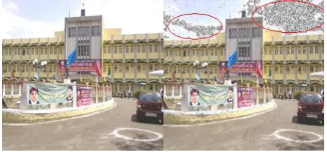
We have also tested the algorithm on wide variety of images and at different noise density levels. During our experiments, we have observed some issues in the images de-noised by MDBUTMF. Some of the images used were landscapes captured on clear sky days with a bright sky in the background. When we processed corrupted versions of these images with MDBUTMF the recovered image resulted in some black patches in the background area.

Figure 1 shows a sample output. The original image is corrupted with 60% additive noise. Then the noisy image is processed using MDBUTMF. As in the figure, the image is recovered to a great extent except the cloudy sky at the top of the image. The effected parts are encircled in do-noised image. The reason for this side effect is when all the pixels in the selected 3 × 3 window are 0 or 255; the noisy pixel is replaced with the mean of the elements in the window. Say at high noise density, 3 out of 9 pixels (in 3 × 3 window) are corrupted, the processing pixel is replaced with the mean the window i.e. 170 (six pixels are 255 and there are 0). It is easy to guess that the pixel being processed is a part of the white background and its corrected value should be 255.

Figure 2.Original & de-noised image (using MDBUTMF)

The problem is not limited to the white patches in the original image. Same issue is observed if the image has some black patches. Figure 2 shows a sample output of this issue. Again the erroneous area is encircled in the de-noise image.

Figure 1. Original & de-noised image (using MDBUTMF)

3.

PROPOSED ALGORITHM

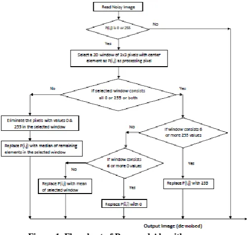
The proposed Improved Decision Based Asymmetric Trimmed Median Filter (IDBATMF) algorithm processes the corrupted images by first detecting the impulse noise. The processing pixel is checked whether it is noisy or noisy free. The pixel is considered as noisy only if it is 0 or 255, all the remaining pixels are left unaltered. If the processing pixel takes the minimum (0) or maximum (255) gray level then it is processed by proposed algorithm. The steps of the IDBATMF are elucidated as follows.

ALGORITHM

Repeat the below steps for each pixel of image.

If selected pixel is other than 0 or 255, it is uncorrupted pixel and it is left unaltered. Else process the pixel.

Step 1: If selected pixel is other than 0 or 255, it is uncorrupted pixel and it is left unaltered. Else process the pixel.

Step 2: Let Pi,j be the pixel being processed. Select a 2-D

window of size 3×3 with Pi,j as the center element.

Step 3: If selected 3×3 window consists of all 0 or 255 or both then

a. If window has 6 or more 255’s then replace Pi,j with 255.

b. Else if window has 6 or more 0’s then replace Pi,j with 0.

c. Else replace Pi,j with mean of elements in the window.

Step 4: If selected window consists of other values as well, then eliminate 0’s and 255’s and find the median of remaining elements. Replace Pi,j with this median value.

As an enhancement to MDBUTMF presented in [9], Step 3a and Step 3b are added in proposed algorithm. MDBUTMF algorithm assumes that all the pixels with 0 or 255 values are noisy and such pixels are replaced. The de-noised image generated by MDBUTMF ensures that there are no pixels with extreme gray level values (0 and 255). Contrary to the assumption made in MDBUTMF, the proposed algorithm suggests that even de-noised image may have some pixel values as 0 or 255 and still be correct. In Step 3a and 3b of the proposed algorithm, we try to identify the regional feature in the image where larger white or black patch may be present in the original image. If such patterns are identified they are handled separately. So the proposed algorithm addresses the issue which was reported in Figure 1 and 2 earlier.

the elements in the window (Step 3c). While in MDBUTMF, the processing pixel is always replaced with the mean of the elements in the window.

In the proposed algorithm, we have used 6 as the threshold value to find out the white or black patches in the image. This threshold value can be parameterized to produce optimum results for different images. It is very important to choose a proper value for this threshold. Let us elaborate how the output will get affected as this threshold value is varied. If the value is increased further, the result of proposed algorithm will be closer to that of MDBUTMF. This will happen because a larger value of threshold would mean that the probability of Step 3a and Step 3b getting executed will decrease and the algorithm will calculate mean of pixels using Step 3c.

Similarly, if the value is decreased then the proposed algorithm will not be able to remove the noise effectively. The reason would be the reverse of the previous case. With smaller threshold value Step 3a and Step 3b will be applied more frequently and more number of noisy pixels will be set as 0 or 255.

A detailed illustration of the proposed algorithm is presented in Section 4. The flowchart of the proposed algorithm is presented in Figure 3.

Figure 1. Flowchart of Proposed Algorithm

4.

ILLUSTRATION OF IDBUTMF

ALGORITHM

As stated in the algorithm, the input (noisy) image is processed pixel by pixel. At each step a window of size 3 × 3 is selected with pixel being processed as the center element. Different cases are illustrated in this section with the help of numerical examples.

In all the examples, selected 3 × 3 window is displayed in a 2-dimentional array. For clarity, the center pixel i.e. the pixel being processed is marked within brackets.

Ex. 1: In this example, the selected window has seven values which are 255 and remaining two values are 0, thus all the pixels in the window are 0 or 255. If we

apply MDBUTMF to this window then the pixel will be replaced with the mean of the elements which is 198. Ex. 2: Let’s find out how this pixel will be handled in

proposed algorithm. Since 7 pixels are 255, it will be processed in Step 3a and processing pixel will be set as 255. As discussed earlier, the assumption is that processing pixel belongs to some white patch in the image, so it is optimum to set the pixel to maximum gray level i.e. white.

Selected window for Ex. 1

Ex. 3: In second example, the selected window has three values which are 255 and remaining six values are 0, again all pixels in the window are 0 or 255. As in Ex. 1, if we apply MDBUTMF to this window then the pixel will be replaced with the mean of the elements which is 85.

Ex. 4: In case of proposed algorithm the pixel will be processed in Step 3b and pixel will be set as 0. This example is exactly opposite to Ex. 1, since six pixel values are 0, the assumption is that the processing pixel belongs to black area in the image, so it is set as minimum gray level i.e. 0.

Selected window for Ex. 2

Ex. 5: In third example, the selected window has five values which are 255 and remaining four values are 0, thus all the pixels in the window are 0 or 255. If we apply MDBUTMF to this window then the pixel will be replaced with the mean of the elements which is 142. Ex. 6: The same result will be obtained by proposed

IDBATMF also because this pixel will be processed by Step 3c of the algorithm. When the distribution of 0’s and 255’s is nearly equal, it is better to use the mean value as suggested in MDBUTMF algorithm.

Selected window for Ex. 3

Ex. 7: In this example there is a mix of 0, 255 and other pixel values. Both MDBUTMF and proposed algorithm process this pixel in the same way. Central pixel is 0, so it is a noisy pixel and needs correction. It will be processed by Step 4 of proposed algorithm.

Ex. 8: Firstly, all 0 and 255 values are trimmed, after trimming only 7 elements are left {170, 210, 176, 220, 188, 198, 80}. The median of these values is 188, so the processing pixel is set to 188.

Ex. 9: Since the pixel being processed 48 is not a noisy pixel, so it is not processed by the algorithm. The value of the pixel remains unchanged.

Selected window for Ex. 5

5.

SIMULATION RESULTS

The existing and proposed algorithms are simulated in MATLAB 7.11 R2010b (32 bit) and tested for various images. De-noising performance of the algorithms is quantitatively measured by PSNR and IEF as in equation (4) and (6) below:

Where PSNR stands Peak Signal to Noise Ratio, MSE stands for Mean Square Error, IEF stands for Image Enhancement Factor, M × N is size of the image, Y represents the original image, denotes the denoised image ƞ represents the noisy image. Execution time of both the algorithms is also computed and compared.

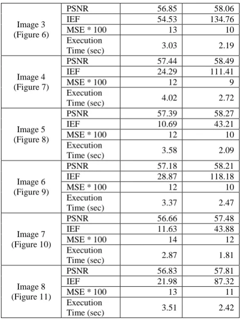
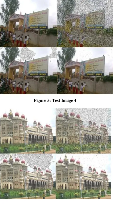
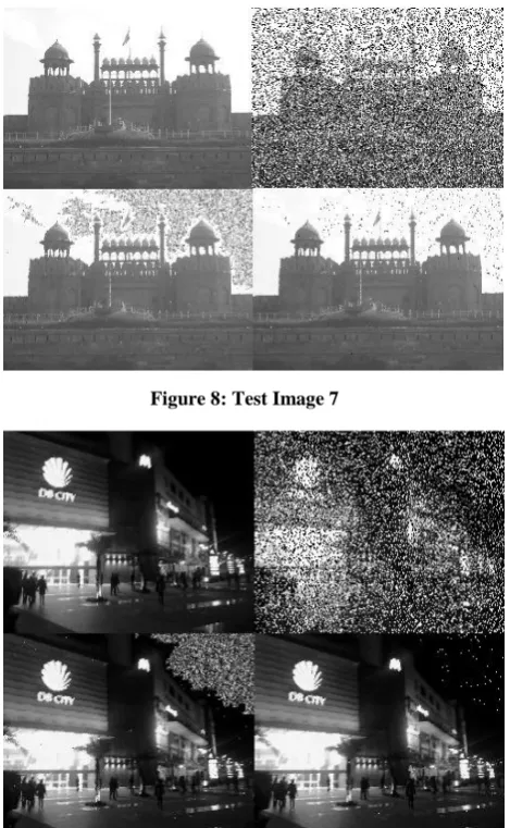
Experiments are performed with a large number of images, consisting of both colored and gray scale images. To compare the performance, the images are corrupted with additive SPN. The density of SPN is varied from 45% to 75% in different images. The images are chosen such that they have a large white or black patch. The corrupted images are restored using both MDBUTMF and the proposed algorithm. MDBUTMF is not able to de-noise such white of black patches effectively but the de-noised images generated by the proposed algorithm show better performance in those patches as well. In this text we have presented the comparative performance for 8 different (Table 1). Figure numbers in first column of the table refers to the experimental results displayed on the next page.

Table 1: Result comparison for test images

Test Image Parameter MDBUTMF Proposed

Algorithm

Image 1 (Figure 4)

PSNR 57.33 58.39

IEF 18.96 65.37

MSE * 100 12 9

Execution

Time (sec) 3.33 2.21

Image 2 (Figure 5)

PSNR 57.19 57.52

IEF 3.70 12.77

MSE * 100 13 12

Execution

Time (sec) 5.58 1.38

Image 3 (Figure 6)

PSNR 56.85 58.06

IEF 54.53 134.76

MSE * 100 13 10

Execution

Time (sec) 3.03 2.19

Image 4 (Figure 7)

PSNR 57.44 58.49

IEF 24.29 111.41

MSE * 100 12 9

Execution

Time (sec) 4.02 2.72

Image 5 (Figure 8)

PSNR 57.39 58.27

IEF 10.69 43.21

MSE * 100 12 10

Execution

Time (sec) 3.58 2.09

Image 6 (Figure 9)

PSNR 57.18 58.21

IEF 28.87 118.18

MSE * 100 12 10

Execution

Time (sec) 3.37 2.47

Image 7 (Figure 10)

PSNR 56.66 57.48

IEF 11.63 43.88

MSE * 100 14 12

Execution

Time (sec) 2.87 1.81

Image 8 (Figure 11)

PSNR 56.83 57.81

IEF 21.98 87.32

MSE * 100 13 11

Execution

Time (sec) 3.51 2.42

As indicated by the simulation results, the performance of proposed algorithm is better on all the parameters. There is a marginal increase in Peak Signal to Noise Ratio (PSNR) in each case. Though visual test of output images is sufficient to compare the de-noising performance of the algorithms, the value of Image Enhancement Factor (IEF) is used to quantify the amount of improvement achieved by the proposed algorithm. It is also interesting to note that along with a remarkable improvement in the quality of recovered image, the proposed algorithm has lower execution time as well. This happens because in Step 3 we do not calculate mean in each case. In step 3a and Step 3b if the selected window consists of more than six 0’s (or 255’s), the processing pixel is set as 0 (or 255). Because of these steps, the time required to calculate mean of elements is saved. In case of MDBUTMF mean is calculated more frequently and hence it takes more time to process the image.

Figure 2: Test Image 1 (Main building of our institute)

Figure 3: Test Image 2 (Apple Wallpaper)

Figure 4: Test Image 3

Figure 5: Test Image 4

Figure 6: Test Image 5

Figure 8: Test Image 7

Figure 9: Test Image 8

6.

CONCLUSION AND FUTURE WORK

In this paper, a new algorithm (IDBATMF) is proposed to restore the images which are corrupted with high density SPN. Most of the existing algorithms used to remove such impulse noise assume that the restored image should not have any pixels with extreme gray level values i.e. 0 or 255. Contrary to this assumption, the proposed algorithm proves that it is possible to have images which actually have pixels with values as 0 or 255. The proposed algorithm tries to identify those pixels and restore them properly. A quantitative comparison of proposed algorithm is also done with the existing noise removal algorithms in terms of PSNR and IEF. The proposed algorithm is simulated in MATLAB 7.11 R2010b (32 bit). The experiments are performed on a system with Intel Core-2-Duo processor and 2 GB RAM. The OS is Windows XP Professional (Service Pack 3). The performance of the algorithm has been tested at varying noise densities on both color and gray-scale images. It is evident from the experimental results that proposed algorithm gives better performance both visibly and quantitatively.

This work can be carried further to improve the quality of the output image. Step 3a and 3b of the algorithm can be improved by increasing the window size to before setting the pixel as 0 or 255. Larger window will help to ensure that the processing pixel actually belongs to some white or black patch of the image. If we increase the window size for the whole algorithm then it may have undesirable blurring effects. Conditional increase of window size will not create blurring effect but may help identify black or whites areas of the image more effectively.

7.

REFERENCES

[1] Gonzalez R., Woods R. “Digital Image Processing” 2/E, Prentice Hall Publisher, 2002.

[2] R. H. Chan, Chung-Wa Ho, M. Nikolova, “Salt and Pepper Noise Removal by Median Type Noise Detectors and Detail Preserving Regularization,” IEEE Transactions on Image Processing, Vol. 14, No.10, pp. 1479-1485, October 2005.

[3] H. Hwang and R. A. Hadded, “Adaptive median filter: New algorithms and results,” IEEE Trans. Image Process., vol. 4, no. 4, pp. 499–502, Apr. 1995.

[4] S. Zhang and M. A. Karim, “A new impulse detector for switching median filters,” IEEE Signal Process. Lett., vol. 9, no. 11, pp. 360–363, Nov. 2002.

[5] P. E. Ng and K. K. Ma, “A switching median filter with boundary discriminative noise detection for extremely corrupted images,” IEEE Trans. Image Process., vol. 15, no. 6, pp. 1506–1516, Jun. 2006.

[6] K. S. Srinivasan and D. Ebenezer, “A new fast and efficient decision based algorithm for removal of high density impulse noise,” IEEE Signal Process. Lett., vol. 14, no. 3, pp. 189–192, Mar. 2007.

[7] V. Jayaraj and D. Ebenezer, “A new switching-based median filtering scheme and algorithm for removal of high-density salt and pepper noise in image,” EURASIP J. Adv. Signal Process., 2010.

[8] K. Aiswarya, V. Jayaraj, and D. Ebenezer, “A new and efficient algorithm for the removal of high density salt and pepper noise in images and videos,” in Second Int. Conf. Computer Modeling and Simulation, 2010, pp. 409–413.

[9] S. Esakkirajan, T. Veerakumar, Adabala N. Subramanyam, and C. H. Prem Chand, “Removal of High Density Salt and Pepper Noise through Modified Decision Based Unsymmetric Trimmed Median Filter”, IEEE Signal Process. Lett., vol. 18, no. 5, May 2011. [10]J. Astola and P. Kuosmanen, Fundamentals of Non

Linear Digital Filtering, BocRaton, CRC, 1997.