http://dx.doi.org/10.4236/gep.2014.23003
How to cite this paper: Tan, S. Q. et al. (2014). A Statistical Model for Long-Term Forecasts of Strong Sand Dust Storms. Journal of Geoscience and Environment Protection, 2, 16-26. http://dx.doi.org/10.4236/gep.2014.23003
A Statistical Model for Long-Term Forecasts
of Strong Sand Dust Storms
Siqi Tan1, Moinak Bhaduri2, Chih-Hsiang Ho2*
1Covance Pharmaceutical Research & Development Co. Ltd, Beijing, China 2Department of Mathematical Sciences, University of Nevada, Las Vegas, USA
Email: *[email protected]
Received February 2014
Abstract
Historical evidence indicates that dust storms of considerable ferocity often wreak havoc, posing a genuine threat to the climatic and societal equilibrium of a place. A systematic study, with empha-sis on the modeling and forecasting aspects, thus, becomes imperative, so that efficient measures can be promptly undertaken to cushion the effect of such an unforeseen calamity. The present work intends to discover a suitable ARIMA model using dust storm data from northern China from March 1954 to April 2002, provided by Zhou and Zhang (2003), thereby extending the idea of em-pirical recurrence rate (ERR) developed by Ho (2008), to model the temporal trend of such sand dust storms. In particular we show that the ERR time series is endowed with the following charac-teristics: 1) it is a potent surrogate for a point process, 2) it is capable of taking advantage of the well developed and powerful time series modeling tools and 3) it can generate reliable forecasts, with which we can retrieve the corresponding mean number of strong sand dust storms. A simula-tion study is conducted prior to the actual fitting, to justify the applicability of the proposed tech-nique.
Keywords
ARIMA Model, Empirical Recurrence Rate, ERR Plot, Point Process, Time Series
1. Introduction
Whimsical and extreme weather patterns have continued to baffle mankind since time immemorial. The past decade has witnessed an unprecedented loss of lives and property primarily due to our inability to adequately foresee weather demons. It’s high time for modelers to come up with new and efficient techniques replacing traditional ones, to tame the grave consequences—a need which is now felt more badly than ever. The focus of the present study would be on one such bane of human civilization: sand storms. But the methods pro-posed can be easily extended to other unforeseen climatic dangers like thunderstorms or hurricanes. Lack of a general consensus among researchers in adequately defining a dust storm leads us to use the following defini-tion due to Tao et al. (2002), specific to Inner Mongolia, China:
Strong dust storm: at least three stations reporting with horizontal visibility of less than 500m and an average wind speed of 17.2 to 24.4 m/s.
Very strong dust storm: at least one station reporting with horizontal visibility of less than 50m and an aver-age wind speed of 20.8 m/s or greater.
These storms can inflict far reaching and grave consequences, including, but not limited to climatic change, chemical and biological alterations in oceans, affecting crop growth and worsening the general survival condi-tions. Neutralization of acid rain is a positive effect that results.
Several climatic factors such as wind, relative humidity, air temperature etc. contribute to the occurrence of these storms and this paper concentrates on storms originating from Hexi Corridor of Gansu Province and Alxa Plateau, southern rim of South Xinjiang Basin and central Inner Mongolia from 1954 to 2002. Thomas T. War-ner (2004), Zhou and Zhang (2003), Yang et al. (2007), and Zhang et al. (2002) provide a gripping account of the changes in their frequency patterns over the last 50 years.
By developing an empirical recurrent rate (ERR) time series, we propose a new treatment to smooth the point process. The ERR is computed sequentially and cumulatively at equidistant time intervals and then we explore the possibility of fitting an ARIMA model to develop reliable and robust forecasts. Designed simulations give valuable insights for building the final model by helping us to mimic the real data.
We intend to proceed as follows: The first section lays out the new definitions we propose, and outlines the rudiments of ARIMA modeling along with rules to help us choose a good model from several competing ones. The next section implements the ideas on a small scale, using a simulated data set, to judge the merit of the pro-posed methods. Encouraged by the success, we next move on to apply similar methods on the real data that we gathered, but firstly using a partitioned version that enables us to test the prediction capabilities and finally, in search of a more reliable and global model, to the entire data set. The necessity of ignoring a few values towards the beginning of the series is highlighted in the section on prediction sets. Encouraging forecasts are obtained throughout the study and finally we briefly detail how can these methods be extended to similar fields.
2. Theory and Method
2.1. Empirical Recurrence Rate
Treating
t
0as the time origin and h as the time step, we generate a time series of the ERR,{ }
zl defined by:(
0 0 no of storms in , ]l l
t t lh n
z
lh lh
+
= = (1)
at the equidistant time intervals t0+h,...,t0+lh,...,t0+Nh ( 0, the present time).= We observe that
{ }
zlevolves over time and is the MLE of the mean, if the underlying process in
(
t t0, 0+lh] is a homogeneous Poisson process. With a forecast horizon of k≥1, we need to predict the value of zt k+ based on the finitehistory:
(
z z1, 2,...,zT)
. The untenable classical regression assumption of the independence of the time evolvingobservations necessitates the introduction of ARIMA models.
2.2. ARIMA Model
A general autoregressive moving average (ARMA) model of order
(
p q,)
is built on the premise that the cur-rent value of a mean zero stationary time series is a linear combination of “p” of its immediate past vales and “q” of its past noise terms and is thus a generalization, embracing the usual AR and MA models. It is thus given by:1 1
p q
t i t i t j t j
i j
X φX− Z θ Z−
= =
−
∑
= +∑
(2)where
{ }
Zt is a Gaussian white noise with mean zero and variance2
σ . The
{ }
1{ }
1
, q
p i i j j
φ = θ
= coefficients are
2) Estimation: We use the maximum likelihood method to estimate the unknown parameters in the model. 3) Diagnostic checking: Tests for normality using the residuals and significance of the model parameters. Honoring the principle of parsimony, we’ll choose the model that has the lowest number of parameters.
2.3. Data Pretreatment
We will use the method of cross validation to partition the data set into two blocks, so that one can be used for model building purposes and the other can be used as refinement tools. In addition, transformations on the data to guarantee stationarity and zero centrality of a time series can be achieved through:
1) Box Cox Transformation: For a given λ and positive observations
(
Y1,...,Yn)
, it is defined as:( )
( )
1
if 0
log if 0
y f y y λ λ λ λ λ − ≠ = = (3)
This transformation helps to stabilize variance, imperative to achieve stationarity. 2) Differencing: A time series
{ }
Xt can be de-trended by considering the dth
order difference, for a suitable
d:
(
1)
dd
t t
X B X
∇ = − (4)
where B is the usual backshift operator.
A lag d difference operator
(
1 d)
dXt Xt Xt d− B Xt
∇ = − = − (5)
can remove the seasonality and trend of period d.
A suspected non-stationarity can be tackled by the transformation and an appropriate order of differencing, which can be dictated by the graph of the ACF function. A quick decay indicates stationarity.
3) Centering: Once stationarity is achieved, we can subtract the sample mean of the transformed data from each observation to get a mean zero process.
2.4. Model Diagnostics
Asymptotically, the sample autocorrelations of an independent and identically distributed sequence
(
Y1,...,Yn)
with finite variance are approximately iid following N 0,1
n
. Thus the usual normal bounds can be used to
check whether the observed residuals are consistent with the iid noise assumption. A statistical test for the ran-domness of the residuals can be done through the well-established Ljung-Box (1978) test statistic. Finally, we can choose between different competing models through the use of the AIC, AICC and BIC criteria.
2.5. Forecasting
Predictions for the future will be achieved from forecasting functions of the form:
(
1,..., 1)
t t t
z = f z− z +a (6)
by forecasting the residuals and then inverting the transformations adopted, to arrive at the forecasts of the original series. Models will be put to test by comparing their generated forecasts with the prediction set and fi-nally, we will combine both the training and the prediction set to obtain reliable forecasts from the chosen model.
2.6. Subset Model Checking
set-tle for a smaller subset model, always lucrative from an interpretative viewpoint. This simpler model, in turn will then be subjected to the usual model selection processes.
3. Simulation Study
The number of monthly sandstorms from March 1954 to April 2002, (Zhou & Zhang, 2003) reviews the pres-ence of too many zeroes in the time series, which questions the justifiability of treating it as a Poisson process. Ensuring stationarity, thus necessitates proper smoothing methods.
Prior to working with the actual data, we intend to investigate the performance of the proposed methods based on a simulated data set, consisting of 17 repetitions of the randomly selected year 1996 from Zhou and Zhang (2003). We converted the data to an ERR time series and used the techniques detailed in the previous section based on a training sample of the first 15 years and a prediction set of the last 2 years.
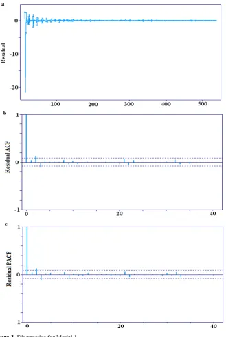
The raw ERR (in 1 month) series was seen to be plagued by significant non-stationarity and periodicity from its sample ACF and PACF graphs. So a Box-Cox transformation (with λ =1.5) and lag 12 differencing were applied and finally, the resulting series was de-trended by an additional lag 1 difference. The ACF and PACF plots (Figure 1) reveal that stationarity is clearly attained. To work with a mean zero model, the sample mean of the transformed data set was subtracted from each observation and an MA(1) model was seen adequate from our initial model search. The estimated (MLE) model is given by:
1 0.1456
t t t
X =Z − Z− (7)
with an estimated white noise variance of 0.049 and a standard error of the MA coefficient as 0.089. Here, Xt
represents a twice-differenced mean corrected time series and Zt represents a white noise process.
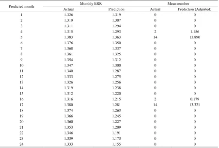
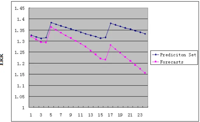
[image:4.595.88.541.413.718.2]The AIC statistic is −25.78 and the Ljung-Box test with a high p-value of 0.94 indicates that the residuals are approximately white noise. That this model is successful from a prediction view point, can be observed from Figure 2. It predicts a mean number of 14 sand storms in April for the two prediction years which is fairly close to the actual number. Table 1 describes this too.
Table 1. Comparison of the actual and predicted ERRs from the simulation study.
Predicted month Monthly ERR Mean number
Actual Prediction Actual Prediction (Adjusted)
1 1.326 1.319 0 0
2 1.319 1.307 0 0
3 1.311 1.294 0 0
4 1.315 1.293 2 1.156
5 1.383 1.363 14 13.890
6 1.376 1.350 0 0
7 1.368 1.337 0 0
8 1.361 1.325 0 0
9 1.354 1.312 0 0
10 1.347 1.300 0 0
11 1.340 1.287 0 0
12 1.333 1.275 0 0
13 1.326 1.256 0 0
14 1.319 1.238 0 0
15 1.312 1.220 0 0
16 1.316 1.215 2 0.179
17 1.380 1.281 14 13.321
18 1.374 1.263 0 0
19 1.366 1.245 0 0
20 1.360 1.227 0 0
21 1.353 1.209 0 0
22 1.346 1.191 0 0
23 1.339 1.173 0 0
Figure 1. Sample ACF and PACF plots showing that stationarity is attained.
Figure 2. Comparison of the observed and predicted ERRs from the simulation study.
4. Real Data Analysis
Using the data source provided by Zhou and Zhang (2003), we intend to carry out similar techniques on the 908 sand storms that occurred in 578 months, from March, 1954 to April 2002, using a time step of 1 month.
4.1. Model Fitting
Attempts to model the sand storm data through ARIMA techniques, by taking the Box-Cox transformation and differencing at lags 12 and 1 failed, since stationarity was difficult to achieve. An ARIMA modeling using a non-cumulative ERR approach proved futile too. Here, we calculated the ERRs for each of the 55 years and were able to reduce the number of zeroes, but since they were calculated independently for each year, there was a huge fluctuation in the series and stationarity was elusive even through the usual transformations.
Thus, we took recourse to the smoothing methods using ERR detailed earlier, dropping the first 13 months, to tame the otherwise widely varying series. It might be observed at this point that a valid data set is an extremely precious component in any modeler’s arsenal and deletion of a subset of it often obscures an otherwise imminent inference. But, in this case, efforts to otherwise circumnavigate this problem of a large initial variance, proved futile. Another justification for the data deletion might be from the relative position of the subset deleted. In real life studies like this, it is only natural for the series to take some time to stabilize and hence the first few errant values are not too likely to exert significant influence on our final inference. We worked with a modified data set of 565 months of sand storms (April 1955-April 2002), where the first 537 formed the training sample and the last 28 played the role of a prediction set. Encouraged by the success of the model it generated, we carried out a similar exercise to the one described with the simulated data set, taking clues from the sample ACF and PACF graphs at each stage and using a Box-Cox transformation (with λ =1.5) and similar lags of 12 and 1, we have our ARMA (1,1) (MLE) model as:
1 1
0.995 0.2688
t t t t
X = X− +Z + Z− (8)
with an estimated white noise variance of 0.29, standard error of AR coefficients as 0.0004 and a standard error of MA coefficients as 0.05.
The AIC statistic was 842.38, but the Ljung-Box test gave a significant p-value of approximately zero, which indicated that the residuals cannot be treated as white noise. We explored the possibility of working with a sim-pler model and found that for the ARMA (1,1) model, the ratio of the AR coefficient was 1.008 and that for the MA coefficient was −0.451 which is less than 1. So a simpler AR(1) model seemed logical and the estimated (MLE) model turned out to be:
1 0.9966
t t t
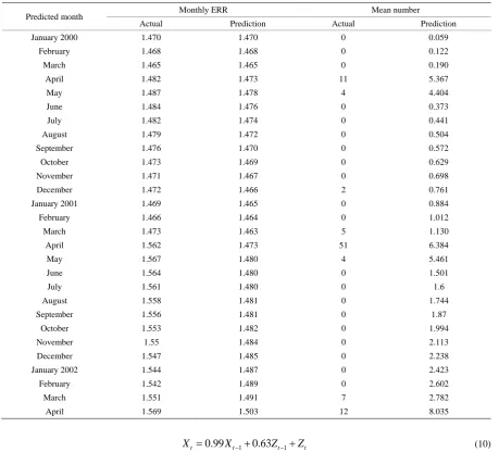
with an estimated white noise variance of 0.29 and a standard error of the AR coefficient as 0.003. This time, the Ljung-Box test gave a non-significant p-value of 0.155, which showed that the residuals are approximately white noise. Figure 3 below confirms this using the appropriate residual plots. Figure 4 shows the comparisons between the actual and predicted ERRs. Table 2 does this comparison too and shows that the ERR predictions are rather close to the actual values.
4.2. Full Data Forecasting
[image:7.595.152.482.220.710.2]Next, we proceeded to combine the training and the prediction set to find a good final model based on all the available 565 points from April 1955 to April 2002. Similar transformations (with the same λ coefficient and lag values) gave the initial estimated ARMA (1, 1) (MLE) model as:
Figure 4. Comparison of the observed and predicted ERRs from Model 1.
Table 2. Comparison of the actual and predicted ERRs from the real data analysis.
Predicted month Monthly ERR Mean number
Actual Prediction Actual Prediction
January 2000 1.470 1.470 0 0.059
February 1.468 1.468 0 0.122
March 1.465 1.465 0 0.190
April 1.482 1.473 11 5.367
May 1.487 1.478 4 4.404
June 1.484 1.476 0 0.373
July 1.482 1.474 0 0.441
August 1.479 1.472 0 0.504
September 1.476 1.470 0 0.572
October 1.473 1.469 0 0.629
November 1.471 1.467 0 0.698
December 1.472 1.466 2 0.761
January 2001 1.469 1.465 0 0.884
February 1.466 1.464 0 1.012
March 1.473 1.463 5 1.130
April 1.562 1.473 51 6.384
May 1.567 1.480 4 5.461
June 1.564 1.480 0 1.501
July 1.561 1.480 0 1.6
August 1.558 1.481 0 1.744
September 1.556 1.481 0 1.87
October 1.553 1.482 0 1.994
November 1.55 1.484 0 2.113
December 1.547 1.485 0 2.238
January 2002 1.544 1.487 0 2.423
February 1.542 1.489 0 2.602
March 1.551 1.491 7 2.782
April 1.569 1.503 12 8.035
1 1
0.99 0.63
t t t t
X = X− + Z− +Z (10)
with an estimated white noise variance of 0.38, the standard errors of the AR and MA coefficients being 0.003
1.4 1.42 1.44 1.46 1.48 1.5 1.52 1.54 1.56 1.58
1 3 5 7 9 11 13 15 17 19 21 23 25 27
[image:8.595.86.546.282.698.2]and 0.033, respectively. But, once again, the Ljung-Box test with a significant p-value of approximately zero re-jects the hypothesis that the residuals are approximately white noise. (AIC = 1051.94). An identical search for a simpler model led us to opt for AR(1) (since the ratio of the MA coefficient in the ARMA (1,1) model was −0.44, a value less than 1) and the estimated (MLE) model was:
1 0.9968
t t t
X = X− +Z (11)
with an estimated white noise variance of 0.47 and a standard error of the AR coefficient as 0.003. A non-significant p-value of 0.75 from the Ljung-Box test now assures that the residuals can be treated as white noise, further confirmation of which was provided by the plots of the residual ACF and PACF (AIC = 1155.07). The forecasts from the full data are shown in Table 3 below.
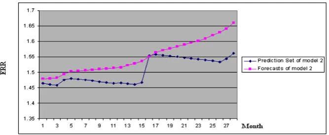
The prediction set plays a pivotal role in model selection, because two models might fit the training data equally well, even with rather different prediction capabilities. This set lets one know the consequences of de-leting the first few data points (where we had high variation), called the burn-in period. To understand this, we recalculate the ERR figures based on the entire data set and delete the first one to arrive at an estimated AR(1) model given by:
1 0.1833
t t t
X = − X− +Z (12)
[image:9.595.89.538.367.721.2]Here, the first 549 points serve as the training set and the last 28 as the prediction set. Defining this as Model 2, we compared its forecasting ability with Model 1 (9), (which was obtained by deleting the first 13 data points), in Figure 4 and Figure 5. The forecasts from Model 1 appear to be more realistic in showing the seasonality of the sand storms in Northern China.
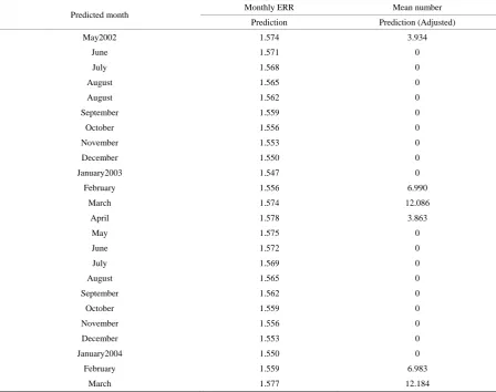
Table 3. Predictions from the final model.
Predicted month Monthly ERR Mean number
Prediction Prediction (Adjusted)
May2002 1.574 3.934
June 1.571 0
July 1.568 0
August 1.565 0
August 1.562 0
September 1.559 0
October 1.556 0
November 1.553 0
December 1.550 0
January2003 1.547 0
February 1.556 6.990
March 1.574 12.086
April 1.578 3.863
May 1.575 0
June 1.572 0
July 1.569 0
August 1.565 0
September 1.562 0
October 1.559 0
November 1.556 0
December 1.553 0
January2004 1.550 0
February 1.559 6.983
Figure 5. Comparison of the observed and predicted ERRs from Model 2.
5. Conclusions
This work successfully finds an acceptable ARIMA model for the sand dust storms occurring in Northern China, through a judicious use of empirical recurrence rates (ERRs). These rates were calculated at equidistant time points and created a useful connection between classical time series and a point process that enabled us to effi-ciently model a random phenomenon that clearly doesn’t follow a Poisson process and hence, otherwise seemed hopelessly intractable, through traditional techniques. We hope that this paper emphasizes the fact that ERR is an effective way to handle a large class of meteorological data that exhibit similar seasonality and we strongly believe that identical ideas can be profitably extended to other fields like biology, economics and social science. It is comforting and encouraging to notice that similar techniques have been profitably used by researchers (e.g., Amei, et al., 2012; Ho, 2010) to model identical natural calamities like large scale earthquakes and volcanic eruptions for long-term predictions. Not onlyshould these evidence provide further confirmation of the applica-bility of this new technique, but should also stimulate serious research investigating fresher avenues like the one proposed.
References
Amei, A., Fu, W., & Ho. C-H. (2012). Time Series Analysis for Predicting the Occurrences of Large Scale Earthquakes. In-ternational Journal of Applied Science and Technology,2, 64-75.
Box, G. E. P., & Jenkins, G. M. (1976). Time Series Analysis: Forecasting and Control. San Francisco: Holden-Day. Brockwell, P. J., & Davis, R. A. (2002). Introduction to Time Series and Forecasting (2nd ed.). New York: Springer-Verlag.
http://dx.doi.org/10.1007/b97391
Cowpertwait, P. S. P., & Metcalfe, A. V. (2009). Introductory Time Series with R. New York: Springer. Cryer, J. D., & Chan, K. S. (2008). Time Series Analysis with Applications in R (2nd ed.). New York: Springer.
http://dx.doi.org/10.1007/978-0-387-75959-3
Goudie, A. S., & Middleton, N. J. (1992). The Changing Frequency of Dust Storms through Time. Climatic Change, 20,
197-225. http://dx.doi.org/10.1007/BF00139839
Ho, C.-H. (2008). Empirical Recurrent Rate Time Series for Volcanism: Application to Avachinsky Volcano, Russia. Jour-nal of Volcanology and Geothermal Research, 173, 15-25.
Ho, C.-H. (2010). Hazard Area and Recurrence Rate Time Series for Determining the Probability of Volcanic Disruption of the Proposed High-Level Radioactive Waste Repository at Yucca Mountain, Nevada, USA. Bulletin of Volcanology,72,
205-219. http://dx.doi.org/10.1007/s00445-009-0309-3
Li, W. K. (2004). Diagnostic Checksin Time Series. Florida: Chapman& Hall/CRC.
Shumway, R. H., & Stoffer, D. S. (2006). Time Series Analysis and Its Applications with R Examples. New York: Springer. Tao, G., Jingtao, L., Xiao, Y., Ling, K., Yida, F., & Yinghua, H. (2002). Objective Pattern Discrimination Model for Dust
Storm Forecasting. Meteorological Applications, 9, 55-62. http://dx.doi.org/10.1017/S1350482702001068
Warner, T. T. (2004). Desert Meteorology. New York: Cambridge University Press.
http://dx.doi.org/10.1016/j.atmosenv.2007.09.025
Zhang, Q. Y., Zhao, X. Y., Zhang, Y., & Li, L. (2002). Preliminary Study on Sand-Dust Storm Disaster and Countermea-sures in China. Chinese Geographical Science, 12, 9-13. http://dx.doi.org/10.1007/s11769-002-0064-2
Zhou, Z. J., & Zhang, G. C. (2003). Typical Strong Sand Storm Events in the Northern China. Chinese Science Bulletin, 48,