A Model of corporate donations to open
source under hardware–software
complementarity
Di Gaetano, Luigi
Department of Economics and Business, University of Catania,
Faculty of Economics, University of Catania
4 July 2012
Online at
https://mpra.ub.uni-muenchen.de/39849/
hardware–software complementarity
Luigi Di Gaetano
July 4, 2012
Abstract In recent years there has been an increasing diffusion of open source projects, as well as an increasing interest among scholars on the topic. Open source software (OSS) is developed by communities of programmers and users, usually sponsored by private firms; OSS is available in the public domain and redistributed for free.
In this paper a model of open and closed source software (CSS) competition will be presented. Hardware and software are complement goods and OSS is financed by hardware firms. There is a differentiated oligopoly of hardware–software bundles, in which firms compete in prices. Results are several; positive (hardware firm) contributions are possible, although, they are not socially optimal. OSS availability has a positive impact on social welfare, and on hardware firms’ profits and prices. CSS firm’s price and profits decrease when OSS is available. The effect on the price of the hardware–CSS bundle depends on demand own–price elasticity.
The model can explain the increasing participation in open source projects of embedded device producers. Hardware firms’ incentives to contribute to OSS development process are greater when there is a relatively intensive competition among producers. Hardware firms use OSS to decrease the software monopolist’s market power.
Keywords Open source·software markets· differentiated oligopoly·complement goods
JEL Classification L17·D21 ·D43·L11
1 Introduction
In recent years there has been an increasing diffusion of open source projects (Lerner and Tirole 2002), as well as an increasing interest among scholars on the topic. Open source software (OSS) is released under a special licence which does not put any restriction on the redistribution of the software and does not require any price, royalty or fee for the use or the redistribution (Rossi 2005;Spiller and Wichmann 2002).
Open source (OS) projects are developed by communities of programmers and users, usually sponsored by private firms; software is available in the public domain and redistributed for free. For an interesting analysis on OSS phenomenon seeSpiller and Wichmann(2002).
Department of Economics and Business University of Catania, Italy
The aim of the paper is threefold. First, the paper analyses competition between open and closed source software, in a market where hardware and software are complements. Second, motivations which determine positive contributions by hardware firms are considered, as well as, conditions for the existence of corporate contributions.
Finally, social welfare analysis will be carried out, to understand the impact of free software on welfare and to asset the efficiency of public intervention instruments, such as transfers to open source and taxation to raise public revenues.
OS software is developed independently by a software foundation, which is financed by hard-ware firms. Exogenous and public donations are also considered. The model is a two stage game with perfect information. In the first stage hardware firms decide the amount of contributions to the OS foundation. These contributions will finance the OSS R&D process. With a certain probability – increasing in the amount of contributions – OSS development will be successful. In second stage, price competition takes place in a differentiated market with hardware and soft-ware bundles. Marginal costs, for both hardsoft-ware and softsoft-ware, are normalised to zero. The basic setting is that ofEconomides and Salop(1992).
The key consideration is that hardware and software are complement goods. The presence of a single monopolist in the software market has a negative effect on hardware firms’ profits. Therefore, vertical and horizontal externalities must be considered (Economides and Salop 1992). Through OSS, hardware firms may increase their prices and profits.
For its characteristics, the model can explain OSS contributions by developers of embedded devices (such as smartphones, tablets, etc.). The relatively small price of these devices, and the complementarity between device and operating system, may constitute an incentive to finance the development of an open source operating system1.
Results are several, positive (private) contributions are possible; although, they are not so-cially optimal. OSS availability has a positive impact on hardware firms’ profits and prices, and on social welfare. CSS firm’s profits and price decrease when OSS is available. The effect on the hardware-CSS bundle’s price depends on model parameters; when demand own–price elasticity is relatively high, the price of CSS–based bundles increases.
The paper is organised as follows. In next section we present the literature background of the paper. Then we develop the model and show theoretical results. Social welfare analysis and instruments for public intervention will follow. Concluding remarks will be presented in the last section.
2 Related literature
Due to the characteristic of public good of OSS, a great deal of attention has been put on moti-vations and incentives of open source project contributors. The analysis of incentives, however, must take into account heterogeneity of developers, contributors and users (Rossi 2005), which could lead to a variety of coexisting motivations.
With regards to the literature, incentives are usually divided in extrinsic and intrinsic motiva-tions2 (Rossi 2005; Krishnamurthy 2006). In the former group, contributions determine present or future external benefits. While motivations in the second group may be associated to a per sepleasure in contributing, such as, for instance, the well known“warm glow” effect (Andreoni
1 Examples of embedded devices’ operating systems, which are open source, are Android by Google,
Maemo/MeeGo by Nokia–Intel, SymbianOS by Nokia, Sony Ericsson and Motorola. For further information seeDorokhova et al.(2009),Anvaari and Jansen(2010) andLin and Ye(2009).
2 On the topic, seeLakhani and Wolf(2005);Hars and Ou(2002);Lakhani and von Hippel(2003);Lerner and
1990). Moreover, motivation analysis must take into account the differences between single indi-viduals and firms.
Lerner and Tirole(2002) focus their attention on programmers’ motivations. They argue that users have three main motivations linked to (1) the need of solving a problem they face (such as program bugs), (2) to benefits from signalling their skills in the job market, and (3) to benefits from peer recognition.
However, some remarks should be moved to these motivations. Reputation incentives, for instance, do not explain the creation of new projects and some activities – for instance, bug reporting, creation and/or translation of software documentation, etc. – which are done by the wide majority of OSS contributors (Rossi 2005).
Krishnamurthy(2006) presents an interesting review of surveys studying motivations in OSS development. Heterogeneity of developers determines a different rank of motivations among them. However, he finds four major factors which influence contributions: financial incentives, nature of task, group size and group structure.
With regards to firm’s motivations, according toWichmann(2002), firms have different po-sitions towards OS project, which depend both on the type of software developed and on the core business of the firm. These motivations may be collocated in four major groups. The first reason may be found on the need of system standardisation. Since OSS is freely available and it can be modified by everyone, it is a good candidate as a common standard3. Furthermore, OS software can be used as a low cost component in bundles, firms can – consequently – use it to increase revenues. Strategic behaviours, such as competition with a dominant firm, and willingness to to enable compatibility between their products and the available software, are the other two incentives.
Two branches of literature must be considered as background for this paper. On the one hand, since hardware and software are complement goods, we have to look at models of competition in complementary markets. Economides and Salop (1992) analyse competition when complement goods may be combined, deriving the equilibrium prices in the market. They also analyse hor-izontal and vertical integration and derive welfare properties. Similarly, Choi (2008) analyses the effects of mergers in markets with complements, when it is possible to sell bundles in the market. Welfare properties of mergers are not clear, they“could entail both pro-competitive and anti-competitive effects” (Choi 2008).
On the other hand, competition between open source and closed source software must be anal-ysed. Several authors examine open/closed source software competition:Bitzer(2004);Bitzer and Schroder (2007); Casadesus-Masanell and Ghemawat (2006); Dalle and Jullien(2003); Econo-mides and Katsamakas(2006);Lanzi(2009);Mustonen (2003);Schmidt and Schnitzer(2003).
Economides and Katsamakas(2006) develop a model of competition in a two–sided market. Firms develop a pricing strategy which takes into account both direct users and other soft-ware firms, the latter produces complementary applications. Main results are that open source availability determines a greater software variety, and in a open/closed source competition“the proprietary system most likely dominates both in terms of market share and profitability”( Econo-mides and Katsamakas 2006).
Dalle and Jullien(2003) analyse competition between MS Windows and Linux in the server operating system market. The presence of network effects – due to compatibility issues between different operating systems – as well as“strong positive local externalities due to the proselytism of Linux adopters” (Dalle and Jullien 2003) are fundamental factors which affect adoption of the new software (Linux). Under certain conditions, adoption of the new technology is fairly rapid.
3 The problem can be referred to the literature which analyses the adoption of different standards. Prisoners’
Windows–Linux competition inspires also the model ofCasadesus-Masanell and Ghemawat (2006). They develop a competition model between software houses, where one product has price equal to zero and cumulative output affects the relative position (due to network externalities). The model, however, is unable to explain the economic behaviour of open source software pro-ducers.
Mustonen (2003) analyses the competitive threat faced by a software monopolist. OSS is developed by programmers. Software prices and monopoly profits decrease – if some conditions are met – under open source software availability.
Schmidt and Schnitzer(2003) develop a model of spatial competition between OSS and CSS firms, where network effects are null, due to perfect compatibility between the two technologies. Users face transportation (adaptation) costs in a Hotelling fashion. Moreover, only a part of the user population can choose what software to adopt; other two groups of users will buy only either OS or CS software. Due to thelock–ineffect, CSS price increases when the number of OSS users increases. Innovation incentives, instead, decrease when OSS users increase in number.
Different results are achieved removing the above assumptions. For instance, Bitzer(2004) develops a Launhardt-Hotelling model of duopoly competition between OSS and CSS. R&D costs to develop OSS are zero. Users heterogeneity, among the different hardware platforms, determines the amount of strategic pressure on CSS price. Moreover,“the absence of development costs for the Linux firm may induce the incumbent to stop any further development of its operating system” (Bitzer 2004).
Bitzer and Schroder(2007), furthermore, analyse the impact of OSS on innovation, in a model where demand depends on technological content of software. Entry of a new OSS firm – from monopoly to duopoly – determines a higher technological level chosen. The result holds whether incumbent is a closed source firm or an open source one. Lower costs for OSS firms in a pure OS competition (i.e. in a duopoly between two OSS firms), as well as higher pay–off for the proprietary software company in a mixed OS–CS competition, determine higher innovation rate than, respectively, mixed competition and pure OS competition.
Lanzi (2009) sets up a two-stage model of quality and price decision, with lock–in effects, externalities due to quality, and perfect compatibility among software platforms. He considers also the accumulated experience of users, which can alter the market structure. He finds two major results. In a duopoly between closed and open source software, CSS price decreases (with respect to monopoly price) if CSS platform is bigger than OSS one and users are experienced. The same result holds if the CSS network is bigger than OSS one, but users have no experience. Under OSS availability the quality of software increases. Finally, given the experience accumulation equation, the ratio of OSS and CSS opportunity costs will define the market structure; which can be either a shared market, or a market where only either OSS or CSS software is available.
3 The model
This paper puts a great deal of attention on companies’ contribution to open source. Comple-mentarity among hardware and software markets, could lead hardware companies to contribute to open source development.
Composite goods (PCS) are sold in a differentiated oligopoly. Hardware and software are fully compatible. The demand system is assumed linear and symmetric, and is equal to the following expressions:
qH1CS=a−bpH1CS+cpH2CS+cpH1OS+cpH2OS qH2CS=a−bpH2CS+cpH1CS+cpH1OS+cpH2OS qH1OS=a−bpH1OS+cpH2CS+cpH1CS+cpH2OS qH1OS=a−bpH2OS+cpH2CS+cpH1OS+cpH1CS
(3.1)
WherepH1CS is the generic price of the PCS composed by hardware produced by firmH1 and
the closed source software. Trivially this price is the sum of the two prices. Due to the nature of open source, however, pOS = 0. The choice of consumers can be interpreted as the decision
of buying a bundle of hardware and CS software or buying only a hardware device and use the freely available software. Consequently, the demand system could be rewritten as in expression (3.2).
qH1CS=a−(b−c)pH1−(b−c)pCS+ 2cpH2 qH2CS=a−(b−c)pH2−(b−c)pCS+ 2cpH1 qH1OS=a−(b−c)pH1+ 2cpCS+ 2cpH2 qH1OS=a−(b−c)pH2+ 2cpCS+ 2cpH1
(3.2)
Cellini et al.(2004) show that the equation system in expression (3.1) is the result of a particular quasi-linear individual utility function. Gross substitutability among all PCS is assumed, this is done by imposing b >3c (Choi 2008). Marginal costs to produce hardware and software are normalised to zero.
Demand for firmi’s product is the sum of all demands for composite goods which contain firmi’s hardware (or software) (Economides and Salop 1992;Choi 2008). So, for instance,qH1 = qH1CS+qH1OS andqCS=qH1CS+qH2CS.
The game is divided in two stages. Perfect information is assumed. In the first stage, there are two hardware firms and a software monopolist. Hardware firms can voluntary contribute to an Open Source Foundation. Companies’ donations are used to finance the open source soft-ware R&D process, they affect the probability of OS softsoft-ware development and release. OSS is successfully developed with probabilityP(FT OT); with FT OT =FH1+FH2+ ¯F. Parameters FH1,FH2 and ¯F are, respectively, hardware firm 1’s donations, firm 2’s donations and exogenous
donations.FT OT represents, therefore, total amount of donations to open source.
The probability P(FT OT) is increasing in donations (i.e. ∂P(FT OT)/∂F > 0), while we
assume the second derivative to be negative. Therefore, we are assuming marginally decreasing returns of R&D investments.
In stage two, two possible outcomes are possible. With probabilityP(FT OT) the open source
software is developed and open source market exists. With opposite probability only closed source market is available. In this stage, price competition will take place.
In the following pages we will consider price competition within the two possible R&D out-comes. Then, results will be compared, together with usual considerations about welfare prop-erties and equilibrium outcomes.
4 Second stage optimisation
4.1 Absence of OS Software
and to take into account substitution path towards other bundles, while maintaining the above system of equations.
When open source market is not released, quantities of OSS–based bundles are zero:
qH1OS=qH2OS= 0 (4.1)
Consequently, the demand system in expression (3.1) can be rewritten as4:
qH1CS =
a(b+c)
b−c −
(b−2c)(b+c)
b−c pH1CS+
c(b+c)
b−c pH2CS
=α−βpH1CS+γpH2CS
qH2CS =
a(b+c)
b−c −
(b−2c)(b+c)
b−c pH2CS+
c(b+c)
b−c pH1CS
=α−βpH2CS+γpH1CS
qH1OS =qH1OS= 0
(4.2)
by imposingα= a(bb−+cc),β =
(b−2c)(b+c)
b−c and γ= c(b+c)
b−c . It should be stressed that, in this way,
substitution paths – towards bundles with CS software – are preserved. In this fashion, part of the demand for the two composite goods is substituted with demand for bundles with CS software. Furthermore, it can be easy to compare the two cases of absence and presence of open source software. As before the system in expression (4.2) can be expressed as follows:
qH1CS=α−βpH1+γpH2−(β−γ)pCS qH2CS=α−βpH2+γpH1−(β−γ)pCS
(4.3)
Property 1 Parameters in the two systems of demands – in absence of OS software, and with OSS – are such thatα > a,β < b,γ > candβ−γ < b−c.
Proof See Appendix A
These results are quite intuitive. The absence of OS software leads to demands for bundles with CS software which have a greater intercept; own price derivative is smaller and cross-product derivative is bigger than the case of OSS availability.
In this case, demands for hardware firms are qHi=qHiCS with i= 1,2, while CS software
company will face a demand equal to the sum of the two.
The generic hardware firm i will maximise its profit function, given that OS software was unsuccessfully developed. Optimisation problem is:
maxpHiqHiCSpHi
maxpHi[α−βpHi+γpHj−(β−γ)pCS]pHi;i, j= 1,2;i6=j
(4.4)
Whose first order condition leads to:
pHi= α
−(β−γ)pCS+γpHj
2β ;i, j= 1,2;i6=j (4.5)
Closed Source monopolist will maximise the following profit function:
maxpCS[qH1CS+qH2CS]pCS
maxpCS[2α−2(β−γ)pCS−(β−γ)(pH1+pH2)]pCS;
(4.6)
4 Results are derived by imposingq
First order condition can be expressed as:
pCS= 2α
−(β−γ)(pH
1+pH2)
4(β−γ) ; (4.7)
From the system of first order conditions, equilibrium prices and quantities are derived. Second order conditions are satisfied due to concavity of the profit functions.
Proposition 1 In absence of open source market, price competition in second stage results in the following equilibrium prices, quantities and profits:
pnos CS =
αβ
(β−γ)(3β−γ); qCSnos= 2 αβ
3β−γ; πnosCS = 2 α2
β2
(β−γ)(3β−γ)2
pnos H1 =p
nos H2 =
α
(3β−γ);q nos H1 =q
nos H2 =
αβ
3β−γ;π nos H1 =π
nos H2 =
α2
β
(3β−γ)2
(4.8)
Proof Equilibrium is derived from the system of first order conditions expressed in (4.5) and (4.7). Equilibrium may also be expressed using original parametersa,bandc(See Appendix B).
4.2 Price competition under OS software availability
With probability P(FH1, FH2,F¯) the open source software is developed. Therefore, a generic
hardware firm will maximise the following profit function:
maxpHi[qHiCS+qHiOS]pHi
maxpHi[2a−2(b−c)pHi+ 4cpHj−(b−3c)pCS]pHi;i, j= 1,2;i6=j
(4.9)
Whose first order condition is:
pHi=2a
−(b−3c)pCS+4cpHj
4(b−c) ;i, j= 1,2;i6=j (4.10)
The maximisation problem for the closed source monopolist is:
maxpCS[qH1CS+qH2CS]pCS
maxpCS[2a−2(b−c)pCS−(b−3c)(pH1+pH2)]pCS;i, j= 1,2;i6=j
(4.11)
Whose first order condition is:
pCS=
2a−(b−3c)(pH1+pH2)
4(b−c) ; (4.12)
As before, equilibrium is derived from the system of first order conditions. Second order conditions are met due to concavity of objective functions.
Proposition 2 Under open source software availability, equilibrium prices, quantities and profits are:
pos CS=
2a(b−c)
(b−3c)(7b−5c)+8c(b−c); q
os CS=
4a(b−c)2
(b−3c)(7b−5c)+8c(b−c); π
os CS=
8a2 (b−c)3 ((b−3c)(7b−5c)+8c(b−c))2
pos H1=p
os H2=
a(3b−c)
(b−3c)(7b−5c)+8c(b−c);qHos1=q
os H2 =
2a(b−c)(3b−c)
(b−3c)(7b−5c)+8c(b−c);πosH1=π
os H2 =
2a2
(b−c)(3b−c)2 ((b−3c)(7b−5c)+8c(b−c))2
(4.13)
4.3 Comparative Statics
Property 2 Under OS availability, hardware prices and profits increase and CS software price decreases,i.e:
pnos
Hi < posHi; i= 1,2
pnos CS > posCS;
πnos
Hi < πosHi; i= 1,2
πnos
CS > πosCS;
(4.14)
The effect onpHiCS (i= 1,2) is not univocally determined. It will increase under OS availability
ifb >14.8214c.
Proof See Appendix D.
Availability of free software leads to several changes in equilibrium prices and quantities. When OS software is developed, the CSS producer competes in a differentiated oligopoly with OS. Therefore, he looses market power. Hardware firms, consequently, may charge a bigger mark– up, leading to higher prices and profits for hardware firms.
OS availability increases hardware producers’ market power, because of two reasons. On the one hand, there is an additional demand for hardware which can be exploited. Secondly, under OSS availability the CS monopolist has to compete in prices with the OSS foundation, the latter produces a software with price equal to zero.
When OS is available, a generic hardware firm faces two markets. In one (HiOS) the hard-ware firm behaves like an integrated firm which produces two complementary products (OSS is freely available, therefore the well-known Cournot problem of double mark-up does not exist). Consequently,pos
HiOS =posHitends to increase with respect topnosHi. In the other market (HiCS),
the CSS producer still charges a mark–up.
In the canonical Cournot problem – with two complementary monopolies – the effect on the overall price (pHiCS) is unambiguous,“joint ownership by a single integrated monopolist reduces
the sum of the two prices, relative to the equilibrium prices of the independent monopolists” (Economides and Salop 1992). In this setting however, prices of PC systems with closed source software may increase. This because there is not joint ownership in the production of CSS-based devices, and also because hardware firms could increase their prices in order to exploit their greater market power under OSS availability.
Whenb is “big enough” (b > 14.8214c) we have that pnos
HiCS < posHiCS. Therefore, when the
own price derivative is relatively big, the effect on hardware price (which increases under OS availability) outweighs the decrease of software price. The overall effect is an increase in the composite good’s price.
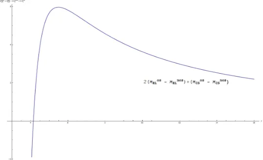
The effect on firms’ profits is unambiguous. Under OS availability, hardware firms increase their profits. The CS producer, on the contrary, is worse off when OSS is realised. This can be seen in Figure n. 1, where the differencesπos
Hi−π
nos Hi andπ
os
CS−πnosCS are depicted as a function
ofx(whereb=xcandx >3).
Fig. 1 Difference in hardware and software firms’ (second stage) profits with regards of OSS availability as functions ofx, withb=xc,x >3,a= 5 andc= 0.35
Fig. 2 Difference the two industries (second stage) profits with regards of OSS availability as function ofx, with b=xc,x >3,a= 5 andc= 0.35
In Figure n. 2 we show the difference of the two industries profits in the two possible outcomes (i.e.2 πos
Hi−π
nos Hi
+ (πos
CS−πCSnos)). As it can be seen, the relationship is not monotonic.
Whenxis relatively small – and, therefore,b→3c– goods tend to be homogeneous. There-fore, the two hardware firms compete almost in a Bertrand fashion, while the CS monopolist has a relatively high market power. The presence of OS software (which has price equal to zero) has a huge effect on profits. The CSS producer, now, has to compete in prices with a virtual firm which commits to a price equal to zero. Then, hardware firms gain a great market power under OSS availability. The more is differentiated the market, the lower is the effect on profits, because losses (of the software monopolist) and gains (of hardware firms) under OSS availability decrease withx.
[image:10.595.79.455.92.268.2] [image:10.595.146.416.316.480.2]be relatively intense (which is equivalent to say, in a two firm case, thatxis small); with open source operating systems, device producers may increase their mark-up and their profits5.
5 First Stage decision
In the first stage, both hardware firms choose the amount of contributions they want to do-nate to the OS foundation. With probabilityP(FT OT) open source software will be successfully
developed, and will be freely available to consumers.
A generic hardware firmimaximises its expected profits decreased by the amount of contri-bution devolved to the OS foundation,i.e.:
F∗
Hi = arg maxFHiP(FT OT)π
os
Hi+ (1−P(FT OT))πnosHi −FHi; i=i,2
F∗
Hi = arg maxFHiπ
nos
Hi +P(FT OT) [πHios −πnosHi]−FHi; i=i,2
(5.1)
The difference πos
Hi−πHinos is positive (Property 2) and is equal to expression (D.3). The first
order condition is:
[πos
Hi−πHinos]
∂P(FT OT)
∂FHi
FHi=FHi∗
= 1; i=i,2 (5.2)
Second order condition is satisfied due to concavity of the probability function, and, consequently, of the profit function. Furthermore, to have a positive amount of contributions, the following condition must be satisfied:
πnos Hi +P(F
∗ H1+F
∗
H2+ ¯F) [π
os
Hi−πHinos]−F ∗
Hi≥πHinos; i= 1,2 (5.3)
According to this condition, hardware firms improve their (expected) profits by contributing to open source software. If this condition is not verified, a positive contribution will not be the market outcome.
6 Consumer Surplus
It is easy to show (See Appendix E) that, under OS availability, consumer surplus is:
CSos= 1 2
" X
∀k
a
b−3c −pk
qk
#
(6.1)
fork={H1CS, H2CS, H1OS, H2OS}.
While, when OS is not developed only two markets exist, and consumer surplus results in the following expression:
CSnos=1 2
" X
∀k
α
β−γ −pk
qk
#
=1 2
" X
∀k
a
b−3c−pk
qk
#
(6.2)
fork={H1CS, H2CS}. This is indeed a special case of the previous expression, where equilib-rium quantities of personal computer systems with open source software are zero.
5 Lin and Ye (2009), for instance, argue that “the price of an OS has a direct impact on device makers’
Proposition 3 Given market outcomes, consumer surplus under OS availability is equal to:
CSos= 4a
2(b−c)3(5b+c)
(b−3c) [(b−3c)(7b−5c) + 8c(b−c)]2 (6.3)
and when OS software is not developed:
CSnos= a
2(b−2c)2(b+c)
(b−c)(b−3c)(3b−7c)2 (6.4)
Property 3 Consumer surplus is greater under OS availability than when OS software is not developed,i.e.CSos−CSnos>0.
Proof See Appendix F
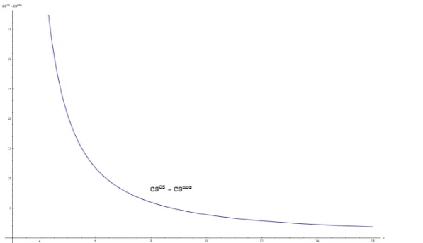
Consumer Surplus increases when OS is available, this is due to the greater variety of goods in the market. Although the price for composite goods which include CS software may increase6, the effect of goods variety outweighed the increase in price in two of the four markets.
Fig. 3 Difference of consumer surplus with regards of OSS availability as function ofx, withb=xc,x >3,a= 5 andc= 0.35
As it can be seen in Figure 3, the difference – which is always positive – in the two consumer surplus decreases with x(given, as before,b =xcand x >3). This means that the presence of OSS determines a relatively small increase in consumer surplus for relatively big values ofx. This because, as seen in Property 2, the price of CSS–based bundles increases when OSS is available for big values of x(x > 14.822), leading to a smaller increase of consumer welfare under OSS availability.
7 First Best Benchmark
Before analysing welfare properties of equilibrium outcomes, it is useful to implement the first best optimum for the game.
[image:12.595.143.442.316.488.2]This special case cannot be implemented, but its derivation is useful to analyse welfare prop-erties of market equilibrium and second best solution.
Total welfare is considered as the unweighed sum of consumer surplus and industries’ profits. In second stage, total welfare is maximised when prices are set equal to marginal costs, which are zero. The ex–ante expected total welfare (and consumer surplus) is maximised by social planner by setting the first best amount of contributions to open source.
Financing OS software is optimal, since consumer surplus under OS availability is bigger than that in the case OSS is not developed, as shown in Proposition 4.
Proposition 4 Imposing all prices to be zero, Consumer Surplus is (with respect to the two R&D outcomes):
CSos F B = 2a
2
b−3c ;CS nos F B =
a2
(b+c)
(b−3c)(b−c) (7.1)
Moreover, CS under OS availability is greater than CS when OS software is not developed, i.e.
CSos
F B> CSF Bnos.
Proof See Appendix G
Also in first best, under OSS availability consumer surplus (and total welfare) is greater than when OSS is not available. This is due to the presence of two more markets when OSS is released. Total welfare corresponds to consumer surplus in this case. In first best, theex–anteexpected total welfare will be maximised7.
F∗
F B= arg max FF B
P(FT OT)·CSF Bos + (1−P(FT OT))·CSF Bnos−FF B (7.2)
whose first order condition is:
[CSosF B−CSF Bnos]
∂P(FT OT)
∂FF B
FF B=FF B∗
= 1 (7.3)
Again, second order condition is satisfied because of concavity of the probability function. Fur-thermore, OS contribution is socially efficient if it improves the (expected) total welfare:
CSF Bnos+P(F ∗
F B+ ¯F) [CSF Bos −CSF Bnos]−F ∗
F B > CSnosF B (7.4)
Since consumer surplus under OS availability is bigger than CSF Bnos, a positive contribution
to OS is optimal (when condition (7.4) is satisfied).
The total amount of contribution is the sum of firms contributions, and considering the symmetric case8, first order condition may be expressed as follows9:
[CSos
F B−CSF Bnos]
∂P(FT OT)
∂FHi
F
Hi=FF B∗ /2
= 1 ;i= 1,2 (7.5)
These conditions are indeed different from companies’ first stage decisions (Expression n. 5.2).
Proposition 5 The level of investment in first best is higher than in the equilibrium outcome.
Proof See Appendix H
Since (hardware) firms consider only private benefits from OSS, and social benefits are greater than private ones, market equilibrium outcome leads to a smaller amount of investment. This comparison, however, is meaningless if in second stage is not possible to impose prices equal to marginal costs (zero). Moreover, in first best, corporate contributions are zero (because profits are zero). Consequently, when first best cannot be reached – as it is assumed in this paper – second best optimum must be derived.
7 Note that in this caseF
T OT =FF B+ ¯F, since ¯F represents exogenous contributions
8 By imposingF
F B=FH1+FH2 andFH1=FH2. ConsequentlyFF B= 2FH1 = 2FH2. 9 Since∂P(F
8 Second best optimum
It is assumed that an intervention on prices is not possible. In second best, total welfare is the sum of consumer surplus, hardware firms’ profits and software producer’s profits. The maximisation problem is10:
F∗
SB = arg max FSB
P(FT OT)·T Wos(1−P(FT OT))·T Wnos−FSB (8.1)
F∗
SB = arg max FSB
T Wnos+P(FT OT) [T Wos−T Wnos]−FSB (8.2)
By imposingFSB=FH1+FH2, first order conditions are derived:
[T Wos−T Wnos] ∂P(FT OT)
∂FHi
F
Hi=FSB∗ /2
= 1 ;i= 1,2 (8.3)
Proposition 6 The level of investment in second best is higher than in the equilibrium outcome, i.e. F∗
SB >2F ∗ Hi.
Proof See Appendix I
The increase in hardware firms’ profits due to the presence of open source software is less than the increase of total welfare, this creates a sub–optimal level of investments with respect to the second best optimum. Moreover, contributing to open source is profitable if and only if, total welfare increases,i.e.:
T Wnos−P(FSB∗ + ¯F) [T Wos−T Wnos]−F ∗
SB≥T Wnos (8.4)
Furthermore, in market equilibrium a positive private contribution may not exist even if it is socially optimal. This happens if the expected OS private gains (increase in hardware firms’ profits) are smaller than investment in OSS development, while social gains – which are bigger than private ones – are greater than F∗
SB. This will be the case, if (See Appendix J):
P(F∗ H1+F
∗ H2+ ¯F) FH∗
i
πHosi−π
nos Hi
<1≤ P(F
∗ SB+ ¯F)
FSB
[T Wos−T Wnos] (8.5)
Given the first order conditions in (5.2) and (8.3), condition (8.5) may be expressed in terms of elasticities as (See Appendix J):
∂P(F∗ SB+ ¯F)
∂FHi
F∗ SB
P(F∗ SB+ ¯F)
≤1< F
∗ Hi
P(F∗ H1+F
∗ H2+ ¯F)
∂P(F∗ H1+F
∗ H2+ ¯F) ∂FHi
(8.6)
That is, the elasticity of the probability function in the market equilibrium is above one, while in second best optimum is smaller than one.
10 It is assumed that the total welfare is the sum of consumer surplus, hardware firm’s profits and CS software
company’s profits,i.e.T Wos=CSos+ 2πos Hi+π
os
CS andT Wnos=CSnos+ 2πHnosi +π
9 Public intervention
9.1 Availability of lump sum tax
Social planner may contribute to Open Source with a subsidy financed by a lump-sum tax. In this way, second best may be reached by a contributionFlstax(and an equal lump sum tax) such
that:
F∗ lstax=F
∗ SB−2F
∗
Hi (9.1)
This contribution permits to reach the second best optimum. The expected total welfare is maximised when:
F∗
lstax= arg max Flstax
T Wnos−P(2F∗
Hi+Flstax+ ¯F) [T W
os−T Wnos]−2F∗
Hi−Flstax (9.2)
SinceF∗
SB is the amount of total contribution which maximises total welfare, imposingF ∗ lstax=
F∗ SB−2F
∗
Hi leads to the second best optimum. It is assumed that this intervention is financed
by a tax which does not create excess of burden of taxation, but note thatF∗
lstax represents the
total amount of revenues raised through the lump sum tax. It is not specified how lump sum tax is divided among agents.
9.2 Contribution financed through corporate income tax
In this section, public contribution to open source is financed by corporate taxes on both hardware and software firms. The model is modified adding a new stage – namely stage zero – in which the social planner sets the tax ratet(witht∈(0,1)) on profits and the amount of public contribution Fctax. Then, first and second stage take place in the same fashion of previous pages.
Price competition (second stage decision) is not affected by the corporate tax, since it does not affect equilibrium prices. Equilibrium profits, however, are a fraction 1−tof previous profits. First stage decision – which refers to private (hardware firms’) donations to open source – is affected by the public intervention, as we will see later. A generic hardware firm will maximise:
Fctax
Hi = arg maxFHi π
nos Hi(1−t)
+P(FHi+FHj+Fctax+ ¯F) [π
os
Hi−πHinos] (1−t)−FHi(1−t)
(9.3)
fori, j= 1,2 andi6=j. First order condition is:
[πHios −πnosHi] (1−t)
∂P(FT OT)
∂FHi
F
Hi=FHictax
= 1−t (9.4)
Finally, social planner maximises the social welfare by setting an optimal tax rate t, and giving a contributionFctax. Contribution must satisfy the budget constraint in expression (9.5).
Fctax=πCSnos+ 2πnosHi +P(2FHctaxi +Fctax+ ¯F) [π
os
CS+ 2πosHi−πCSnos−2πnosHi]−2FHctaxi t (9.5)
Therefore the tax rate may be expressed in the following fashion:
t= Fctax
πnos
CS + 2πnosHi +P(2FHctaxi +Fctax+ ¯F) [π
os
CS+ 2πosHi−πCSnos−2πnosHi]−2FHctaxi
Finally, the social maximisation problem is:
F∗
ctax= arg maxFctax [CS
nos+ (πnos
CS + 2πHinos) (1−t)]
+P(2Fctax
Hi +Fctax+ ¯F) [CS
os+ (πos
CS+ 2πosHi) (1−t)
−CSnos−(πnos
CS + 2πHinos) (1−t)]−2FHctaxi (1−t)−Fctax+Fctax
(9.7)
It easy to show that the above maximisation problem is equivalent to the following problem (see Appendix K):
F∗
ctax= arg maxFctaxT W
nos+P(2Fctax
Hi +Fctax+ ¯F) [T W
os−T Wnos]
−2Fctax
Hi −Fctax
(9.8)
As before, imposing 2Fctax
Hi +Fctax=F
∗
SBleads to the second best outcome, therefore the optimal
public contribution will be:
F∗ ctax=F
∗
SB−2FHctaxi (9.9)
and the optimal tax rate will be calculated accordingly using expression (9.6).
Property 4 Under corporate income taxation, the amount of private contributions is smaller than the equilibrium outcome without public intervention,i.e.F∗
Hi> FHictax.
Proof See Appendix L.
Income tax and public transfers to the OS Foundation create a distortion in the amount of private contributions. Public intervention has a crowding out effect on private investments in OSS. Despite this distortion in private contributions, second best optimum can be reached also without a lump sum tax by imposing a certain tax rateton firms’ profits. However, the optimal corporate income tax rate t∗
should be less than – or equal to – 1 (t∗
≤1). From expression (9.6), this means that:
πnosCS + 2πHinos+P(2FHctaxi +Fctax+ ¯F) [π
os
CS+ 2πHios −πCSnos−2πnosHi]−2FHctaxi ≥F
∗
ctax (9.10)
πCSnos+ 2πnosHi +P(2FHctaxi +Fctax+ ¯F) [π
os
CS+ 2πosHi−πCSnos−2πHinos]≥F ∗
SB (9.11)
Expected profits of the two industries (the left hand side of expression (9.11)) must be greater than the optimal total second best contribution. Indeed this is needed because public contribu-tions to the OSS foundation will be raised using industries’ profits .
So, although corporate income tax may be optimal (in second best), there could be cases where second best optimum cannot be reached using this instrument.
10 Conclusions
This paper contributes to the growing literature regarding open source phenomenon. In this model, the complementarity between hardware and software provides an incentive for hardware firm contribution to OSS development.
OSS release has two major positive consequences in our model. On the one hand, the absence of OSS determine a lower welfare, since there are consumers who may prefer OSS bundles rather than CSS-based PCS. Only some of them substitute their consumption of personal computer systems with CSS-based bundles. On the other hand, since open source is free, the problem of double mark-up is partially solved (in two out four markets). Furthermore, price competition for software is more intense, due the public availability of OSS. Therefore, OSS development has always a positive impact on total welfare.
Hardware firms – under the non negativity condition – contribute positively to the devel-opment of open source software. This contribution, however, is not optimal with respect to the second best benchmark. Second best can be reached with a lump sum tax, and with a corporate income tax. With the latter instrument, however, second best may not be a feasible point if the two industries’ profits are less than the optimal second best total contribution.
This model may explain the recent development of several open source operating systems for embedded devices (such as tablets, smartphones, netbooks, etc.), since hardware firms incentives increase when the market is relatively homogeneous.
A limit of the model is that the decision of contributing to the open source foundation is exogenously given. It can be the case that hardware firms can decide to develop their own closed source operating system. With OSS, however, R&D development has greater chances of being successful, since donations by firms (as well as exogenous and public contributions) jointly increase the probability of software development.
Other critical points are the assumption of compatibility of hardware and software, as well as the assumed symmetric demand for CSS and OSS bundles. Future developments may consider the interaction between a greater number of software companies, as well as differences in the quality of software.
References
James Andreoni. Impure Altruism and Donations to Public Goods: A Theory of Warm-Glow Giving. The Economic Journal, 100(401):464 – 477, 1990.
Mohsen Anvaari and Slinger Jansen. Evaluating architectural openness in mobile software platforms. In Proceed-ings of the Fourth European Conference on Software Architecture: Companion Volume, ECSA ’10, pages 85 – 92, New York, NY, USA, 2010. ACM.
Jurgen Bitzer. Commercial versus Open Source Software: The Role of Product Heterogeneity in Competition.
Economic Systems, 28(4):369 – 381, 2004.
Jurgen Bitzer and Philipp J. H. Schroder. Open Source Software, Competition and Innovation. Industry & Innovation, 14(5):461–476, 2007.
Ramon Casadesus-Masanell and Pankaj Ghemawat. Dynamic Mixed Duopoly: A Model Motivated by Linux vs. Windows. Management Science, 52(7):1072–1084, 2006.
Roberto Cellini, Luca Lambertini, and Gianmarco I.P. Ottaviano. Welfare in a differentiated oligopoly with free entry: a cautionary note. Research in Economics, 58(2):125 – 133, 2004.
Jay P. Choi. Mergers with Bundling in Complementary Markets. The Journal of Industrial Economics, 56(3): 553 – 577, 2008.
Jean-Michel Dalle and Nicolas Jullien. ‘Libre’ software: turning fads into institutions? Research Policy, 32(1):1 – 11, 2003.
Regina Dorokhova, Nickolay Amelichev, and Kirill Krinkin. Evaluation of Modern Mobile Platforms from the Developer Standpoint. St. Petersburg Electrotechnical University, Open Source and Linux Lab (OSLL), 2009. Nicholas Economides and Evangelos Katsamakas. Two-Sided Competition of Proprietary vs. Open Source Tech-nology Platforms and the Implications for the Software Industry. Management Science, 52(7):1057–1071, 2006.
Nicholas Economides and Steven C. Salop. Competition and Integration Among Complements, and Network Market Structure. The Journal of Industrial Economics, 40(1):105 – 123, 1992.
Sandeep Krishnamurthy. On the intrinsic and extrinsic motivation of free/libre/open source (FLOSS) developers.
Knowledge, Technology & Policy, 18:17–39, 2006.
Karim R. Lakhani and Eric von Hippel. How Open Source software works: “Free” user-to-user assistance.Research Policy, 32:923–943, 2003.
Karim R. Lakhani and Robert G. Wolf. Why Hackers Do What They Do: Understanding Motivation and Effort in Free/Open Source Software Projects. In Joseph Feller, Brian Fitzgerald, Scott A. Hissam, and Karim R. Lakhani, editors,Perspectives on Free and Open Source Software, chapter 2, pages 15–55. MIT Press, 2005. Diego Lanzi. Competition and Open Source with Perfect Software Compatibility. Information Economics and
Policy, 21(3):192 – 200, 2009.
Josh Lerner and Jean Tirole. Some Simple Economics of Open Source. Journal of Industrial Economics, 50(2): 197 – 234, 2002.
Josh Lerner and Jean Tirole. The Economics of Technology Sharing: Open Source and Beyond. Journal of Economic Perspectives, 19(2):99–120, 2005.
Feida Lin and Weiguo Ye. Operating System Battle in the Ecosystem of Smartphone Industry. InInformation Engineering and Electronic Commerce, 2009. IEEC ’09. International Symposium on, pages 617 – 621, may 2009.
Mikko Mustonen. Copyleft – the economics of Linux and other open source software. Information Economics and Policy, 15(1):99–121, 2003.
Maria Alessandra Rossi. Decoding the Free/Open Source Software Puzzle: A Survey of Theoretical and Empirical Contributions. In Jürgen Bitzer and Philipp J.H. Schröder, editors,The Economics of Open Source Software Development, chapter 2, pages 15–55. Elsevier, 2005.
Klaus M. Schmidt and Monika Schnitzer. Public subsidies for open source? Some economic policy issues of the software market.Harvard Journal of Law and Technology, 16(2):473 – 502, 2003.
Dorit Spiller and Thorsten Wichmann. Basics of F/OSS software markets and business models. InFree/Libre and F/OSS Software: Survey and Study, FLOSS Final Report, chapter 3. International Institute of Infonomics, Berlecom Research GmbH, 2002.
Thorsten Wichmann. Firms’ Open Source Activities: Motivations and Policy Implications. In Free/Libre and F/OSS Software: Survey and Study, FLOSS Final Report, chapter 2. International Institute of Infonomics, Berlecom Research GmbH, 2002.
Appendix
Note that Proof usingMathematicaare available in a separate document, which can be released on request by the author.
A Proof of Property 1
It can be easily shown that the following inequalities hold:
α=ab+c
b−c> a, since b+c b−c >1;
β=(b−2bc)(b+c)
−c < b, since (b−2c)(b+c)< b(b−c) ⇐⇒ 2c
2>0;
γ=cb+c
b−c> c, since b+c b−c>1;
β−γ=(b−3bc)(b+c)
−c < b−c, since (b−3c)(b+c)<(b−c)
2 ⇐⇒ 4c2>0.
B Equilibrium when OSS is not released
Equilibrium, when OSS is not available, (expression n. 4.8) may also be expressed using original parametersa,b andc:
pnos CS =
a(b−2c)
(b−3c)(3b−7c); qnosCS = 2
a(b+c)(b−2c)
(b−c)(3b−7c); πCSnos= 2
a2(b+c)(b−2c)2 (b−c)(3b−7c)2(b−3c)
pnos H1 =p
nos H2 =
a
(3b−7c);q
nos H1 =q
nos H2 =
a(b+c)(b−2c) (b−c)(3b−7c);π
nos H1 =π
nos H2 =
a2
(b+c)(b−2c) (b−c)(3b−7c)2
Furthermore, due to the market structure, the following equalities hold true:qnos H1CS =q
nos H2CS =q
nos H1 =q
nos H2 = 1
2q
nos CS and:
pnos H1CS=p
nos H2CS=p
nos H1 +p
nos
CS =pnosH2 +p
nos CS =
a(2b−5c)
(b−3c)(3b−7c) (B.2)
C Equilibrium quantities for composite goods under OS availability
Given maximisation problems in expressions (4.9) and (4.11), the system of first order conditions leads to the following equilibrium quantities – and prices – for the personal computer systems (composite goods):
qos
H1CS=qosH2CS=
2a(b−c)2 (b−3c)(7b−5c)+8c(b−c)
qos
H1OS =qosH2OS=
4ab(b−c) (b−3c)(7b−5c)+8c(b−c)
pos
H1CS=posH2CS=
a(5b−3c) (b−3c)(7b−5c)+8c(b−c)
pos
H1OS =posH2OS=
a(3b−c) (b−3c)(7b−5c)+8c(b−c)
(C.1)
Expressing quantities and prices in this fashion is useful to compute consumer surplus.
D Proof of Property 2
Due to symmetry of demand functions, prices and quantities for the two hardware companies are equal. The first inequality is always satisfied11:
pos
Hi−pnosHi >0
=(b−3c)(7ab−(3b−c5c)+8) c(b−c)−3b−a7c
=a(3b−c)(3b−7c)−(b−3c)(7b−5c)−8c(b−c) (3b−7c)((b−3c)(7b−5c)+8c(b−c))
=a(3b−7c)((b−23bc()(7b−b−3c5)c)+8c(b−c))>0
(D.1)
CS software price decreases when OS software is available,i.e.: pnos
CS −p os CS >0
=(3b−a(7b−c)(2b−c)3c)−(b−3c)(72b−a(b−c5c)+8) c(b−c)
=a(b−2c)(b−3c)(7b−5c)+8c(b−2c)(b−c)−2(b−c)(3b−7c)(b−3c) (3b−7c)(b−3c)[(b−3c)(7b−5c)+8c(b−c)]
=a(b−3c)(b+c)(b−c)+c[(b−3c)2+8(b−2c)(b−c)]
(3b−7c)(b−3c)[(b−3c)(7b−5c)+8c(b−c)] >0
(D.2)
Hardware firms’ profits (without considering R&D costs) increase when OS is available, and CS software producer’s profits decrease when OS software is available, therefore:
πos
Hi−πHinos =
2a2
(b−c)(3b−c)2 [(b−3c)(7b−5c)+8c(b−c)]2 −
a2
(b+c)(b−2c) (3b−7c)2(b−c) >0
πnos
CS −πosCS = 2
a2(b+c)(b−2c)2 (b−c)(3b−7c)2(b−3c)−
8a2(b−c)3
((b−3c)(7b−5c)+8c(b−c))2 >0
(D.3)
Due to complexity of the polynomials, the computational software Mathematica is used to verify these two conditions; which are always true forb >3c,a >0 andc >0. Finally, the difference in the price of PC systems with CS software, with or without OS software, is:
pnos
HiCS−posHiCS=
a(2b−5c) (b−3c)(3b−7c)−
a(5b−3c)
(b−3c)(7b−5c)+8c(b−c) (D.4)
Again, usingMathematica,pnos
HiCSis greater thanp os
HiCS ifb3+ 49bc2<18b2c+ 28c3or, equivalently,:
pnos
HiCS> posHiCS ⇐⇒ b2(b−18c) +c2(49b−28c)<0 (D.5)
Imposingb=xcwithx >3, the inequality in expression (D.5) can be rewritten asc3
x2(x−18) + 49x−28 <0. The parameter c is greater than zero by assumption. The polynomial in the square brackets is equal to zero (x2(x−18) + 49x−28 = 0) whenxassumes the following values:
{{x→0.791373},{x→2.38719},{x→14.8214}} (D.6)
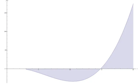
In the interval of our interest,i.e.forx >3, the polynomial is smaller than zero (x2(x−18) + 49x−28<0) for x <14.8214. While is greater than zero whenx >14.8214. This can be seen in Figure 4.
Fig. 4 Plot off(x) =x2(x−18) + 49x−28 for valuesx >3
Whenb is “big enough” (b >14.8214c) thenpnos HiCS < p
os
HiCS. Therefore, when the own price derivative is
relatively big, the effect on hardware price (which increases under OS availability) outweighs the decrease of CSS price. The overall effect is an increase in the composite good’s price.
E Consumer surplus
The system of equation in expression (3.1) shows demands as a function of prices. In the following expression (E.1), the system is rewritten in order to have prices as a function of quantities:
pH1CS=
a b−3c−
b−2c
(b−3c)(b+c)qH1CS−
c
(b−3c)(b+c)[qH2CS+qH1OS+qH2OS] pH2CS=
a b−3c−
b−2c
(b−3c)(b+c)qH2CS−
c
(b−3c)(b+c)[qH1CS+qH1OS+qH2OS] pH1OS=
a b−3c−
b−2c
(b−3c)(b+c)qH1OS−
c
(b−3c)(b+c)[qH2CS+qH1CS+qH2OS] pH1OS=
a b−3c−
b−2c
(b−3c)(b+c)qH2OS−
c
(b−3c)(b+c)[qH2CS+qH1OS+qH1CS]
(E.1)
[image:20.595.136.418.299.470.2]F Proof of Property 3
UsingMathematicait is easy to verify that the following expression holds true fora >0,b >3candc >0:
CSos−CSnos= 4a2 (b−c)3
(5b+c)
(b−3c)[(b−3c)(7b−5c)+8c(b−c)]2 −
a2 (b−2c)2
(b+c)
(b−c)(b−3c)(3b−7c)2 >0 (F.1)
G Proof of Proposition 4
When OS software is not available, and prices are zero, quantities demanded areqH1CS=qH2CS=α. Therefore
the consumer surplus is:
CSnos F B =
1 2·2
α β−γ−0
α=β−γα2 = a 2
(b+c)
(b−c)(b−3c) (G.1)
Industries’ profits are zero. Equivalently, under OS availability, qH1CS = qH2CS = qH1OS = qH2OS = a.
Consumer surplus is:
CSos F B=
1 2·4
a b−3c−0
a= 2a2
(b−3c) (G.2)
The difference between the two surpluses is:
CSos F B−CS
nos F B =
2a2
(b−3c)−
a2 (b+c) (b−c)(b−3c) =
a2
b−c (G.3)
which is trivially greater than zero, as stated in the Proposition.
H Proof of proposition 5
First order conditions, respectively, in market equilibrium and in first best are shown in expression (5.2) and (7.5). Since the second derivative of the probability function is negative, there is a smaller amount of investment with respect to the first best if:
∂P(FT OT)
∂FHi
market
> ∂P(FT OT)
∂FHi
F B
;i= 1,2 (H.1)
Which is equivalently to say that the first derivative ofP(·) in the market outcome is greater than that in First best (with prices equal to zero). This condition can be rewritten as follows (at optimum):
1
πos i −πnosi
> 1
CSos F B−CSnosF B
;i= 1,2
CSos
F B−CSF Bnos−
πos
i −πnosi
>0 ;i= 1,2 (H.2)
Using the computational software, it can be easily seen that this condition is satisfied fora >0,b >3c >0.
I Proof of proposition 6
In the same fashion of the previous proof, it is necessary to demonstrate that:
∂P(FT OT)
∂FHi
market
> ∂P(FT OT)
∂FHi
SB
;i= 1,2 (I.1)
Which corresponds to the following inequality (at optimum):
1
πos i −πinos>
1
T Wos−T Wnos ;i= 1,2
CSos+ 2πos Hi+π
os CS− CS
nos+ 2πnos Hi +π
nos CS
−πos i −π
nos i
>0 ;i= 1,2 (I.2)